Qualitative Analysis of a Single-Species Model with Distributed Delay and Nonlinear Harvest

Abstract

In this paper, a single-species population model with distributed delay and Michaelis-Menten type harvesting is established. Through an appropriate transformation, the mathematical model is converted into a two-dimensional system. Applying qualitative theory of ordinary differential equations, we obtain sufficient conditions for the stability of the equilibria of this system under three cases. The equilibrium $A_1$ of system is globally asymptotically stable when $br-c>0$ and $\eta <0$. Using Poincare-Bendixson theorem, we determine the existence and stability of limit cycle when $br-c>0$ and $\eta >0$. By computing Lyapunov number, we obtain that a supercritical Hopf bifurcation occurs when $\eta$ passes through 0. High order singularity of the system, such as saddle node, degenerate critical point, unstable node, saddle point, etc, is studied by the theory of ordinary differential equations. Numerical simulations are provided to verify our main results in this paper.

1. Introduction

Single-species is a unit of the whole ecosphere. Although most biological populations are multi-species, there is no single population in the strict sense, but because of artificial breeding, there are a lot of single population resources in many human-created environments, which provide indispensable roles for human production and life. Due to the economic interests and production needs, people need to develop the single population resources for a long time and continuously, and to give full play to the best use value on the basis of the lowest cost consumption as possible, so the control and prediction of the single population is particularly important.

Single-species models are widely used in the field of mathematical biology, such as pest management, optimal management of biological resources, epidemic prevention and control, cell growth regulation and so on. Many scholars (see [1,2,3]) have obtained some good properties of these models by quantitative analysis, and the results help us forecast and control the actual production. Wang et al. [4] studied a single-species model and found an optimal harvesting strategy which allows the output to reach a maximum and remains constant. At the same time, the population quantity can attain the maximum level in a precise time interval when the population has been harvested. Dou et al. [5] addressed a non-autonomous Logistic single-species model. The analytical expressions about the best harvesting strategy have been obtained by Pontryagin control and optimization principles of impulsive systems. Recently, many articles have also focused on the study of single-species population model (see [6,7,8,9]).

We know that both discrete and distributed delays tend to bring more rich and complex dynamics to a population dynamic system. For researchers, although models with delay are more complex than without delay, the research results of these models are closer to actual life. In 1948, Hutchinson [10] analyzed a Logistic delay equation characterizing animal populations, and the form is

$$\frac{\mathrm{d}x\left(t\right)}{\mathrm{d}t}=rx\left(t\right)\left(1-\frac{x(t-\tau )}{K}\right),$$

(1)

which could vividly simulate the population size. In (1), the food supply at time t depends on the population number at time $t-\tau$. More generally, many scholars studied some models in which the current population density continuously depends on the population density in the past period. For example, Cushing [11] proposed the following single population model with distributed delay

$$\frac{\mathrm{d}x\left(t\right)}{\mathrm{d}t}=rx\left(t\right)\left(-1-ax\left(t\right)-\omega {\int }_{-\infty }^t{k}_1(t-s)x\left(s\right)\mathrm{d}s\right),$$

(2)

and detailed qualitative results were obtained. Pang et al. [12] considered the following single population model with distributed delay and impulsive state feedback control

$$\left\{\begin{array}{c}\frac{\mathrm{d}x\left(t\right)}{\mathrm{d}t}=rx\left(t\right)[1-cx\left(t\right)-\omega {\int }_{-\infty }^{t}exp\left(a(t-s)\right)x\left(s\right)\mathrm{d}s],x\left(t\right)<h,\hfill \\ \mathrm{\Delta }x\left(t\right)=-\beta x\left(t\right),x\left(t\right)=h,\hfill \end{array}\right.$$

(3)

and sufficient conditions for the existence and stability of the order-1 periodic solution and limit cycles were obtained, where $\mathrm{\Delta }x\left(t\right)=x\left(t^{+}\right)-x\left(t\right)$. Ruan and Wolkowicz [13] built a chemostat model about single population with distributed delay, and they obtained that the system existed Hopf bifurcations by taking the average time delay as the bifurcation parameter. Lian et al. [14] considered a predator-prey system with Holling type IV functional response and time delay. They studied the effects of time delay on this system and obtained the conditions of local asymptotic stability of the positive equilibrium and the existence of local Hopf bifurcations by applying the delay as a bifurcation parameter. Yao et al. [15] investigated the global asymptotic stability of fractional-order complex-valued differential equations with distributed delays. Based on the Laplace transform method, a novel necessary and sufficient condition for the stability is established by embedding the characteristic equation into a two-dimensional complex system. The algebraic criterion is expressed by the fractional exponent, coefficients, and the delay. Many single-species population models with time delay were studied and rich results were obtained (see [16,17,18,19,20,21,22]).

In addition, many scholars have studied the single population model with different forms of harvest. Clark [23] introduced the following single population model with linear harvest,

$$\frac{\mathrm{d}x\left(t\right)}{\mathrm{d}t}=rx\left(t\right)\left(1-\frac{x\left(t\right)}{K}\right)-Ex\left(t\right).$$

(4)

Clark introduced the single population model (4) with linear harvest, analytical expressions for optimal harvest of a renewable resource stock, which is subject to a stochastic process are found. These expressions give the optimal harvest as an explicit feedback control law. All relations in system (4), including the stochastic process, may be arbitrary functions of the state variable (stock). In 1978, Ludwig et al. [24] put forward the following single population model with nonlinear harvest,

$$\frac{\mathrm{d}N}{\mathrm{d}t}=r_B\left(1-\frac{N}{K_B}\right)-\frac{B{N}^2}{A^2+N^2}.$$

(5)

Nonlinear harvesting has been proposed and some novel conclusions have been obtained. Tan et al. [25] considered the following single population system with implusive disturbance and nonlinear harvest:

$$\left\{\begin{array}{c}{\displaystyle \frac{\mathrm{d}x\left(t\right)}{\mathrm{d}t}=x\left(t\right)[a\left(t\right)-b\left(t\right)x\left(t\right)]-\frac{c\left(t\right)x\left(t\right)}{d\left(t\right)+x\left(t\right)},t\ne {\tau }_k,k\in \mathbb{N},}\hfill \\ x\left({\tau }_k^{+}\right)=(1+{\lambda }_k)x\left({\tau }_k\right).\hfill \end{array}\right.$$

(6)

They obtained good dynamic properties. Li et al. [26] established and analyzed a single-species model with delay weak kernel and constant rate harvesting:

$${\displaystyle \frac{\mathrm{d}x\left(t\right)}{\mathrm{d}t}=rx\left(t\right)\left(1-\frac{1}{K}{\int }_{-\infty }^t\alpha e^{-\alpha (t-s)}x\left(s\right)\mathrm{d}s\right)-u.}$$

(7)

The existence of the equilibrium point of the model (7) is obtained, and the properties of the positive equilibrium state of the population are studied.

Population model with distributed delay and harvest plays an important role in ecosystem, which can reflect the growth rule of invertebrate population better and help us get the best policy of harvesting. This paper is mainly aimed at qualitative analysis of a single-species population model with distributed delay and nonlinear harvest. By the establishment of a single-species population model of differential equations, and using stability analysis methods to discuss the existence and stability of equilibria of the system, we can forecast the development of the population.

The rest of this paper is organized as follows. In Section 2, we establish a single-species model with distributed delay and nonlinear harvest and make a statement about the model. Then, we will discuss the existence and stability of the equilibria of the system under three different cases from Section 3, Section 4 and Section 5. In Section 6, we verify our results by numerical simulations. The conclusions will be given in Section 7.

2. The Model

We combine distributed delay and nonlinear harvest to consider a new single-species model. From biological and economic points of view, Michaelis-Menten type harvesting is more realistic among the several types of harvesting. Thus, a single-species model with distributed delay and Michaelis-Menten type harvesting is established as follows:

$$\frac{\mathrm{d}x\left(t\right)}{\mathrm{d}t}=x\left(t\right)\left(r-\omega {\int }_{-\infty }^t\alpha exp(-\alpha (t-s))x\left(s\right)\mathrm{d}s\right)-\frac{cx\left(t\right)}{b+x\left(t\right)},x\left(t\right)\ge 0,$$

(8)

where $x\left(t\right)$ denotes the density of the population at time t, r denotes the intrinsic rate of increase of the population, $\omega ,\alpha ,b$ and c are positive constants. ${\int }_{-\infty }^t\alpha exp(-\alpha (t-s))x\left(s\right)\mathrm{d}s$ indicates the impact of distributed time delay. The term ${\int }_{-\infty }^t\alpha exp(-\alpha (t-s))x\left(s\right)\mathrm{d}s$ represents the effect of distributed delay from the following aspects: The integral for s from $-\infty$ to t represents the continuous influence on current state $x\left(t\right)$ from the past time, which shows the influence interval for distributed delay. That is, the entire interval from the past to current time t has impact on current state $x\left(t\right)$. The kernel function $\alpha exp(-\alpha (t-s\left)\right)(s\in [0,\infty \left)\right)$ represents the influential degree to current state $x\left(t\right)$ from time s to t. $x\left(s\right)(s\in (\infty ,t\left]\right)$ represents the density of population at the past time s. Therefore, the term $\omega {\int }_{-\infty }^t\alpha exp(-\alpha (t-s))x\left(s\right)\mathrm{d}s$ represents the distributed delay in the model. $\frac{cx\left(t\right)}{b+x\left(t\right)}$ is simplified Michaelis-Menten type harvesting (the details of this kind of harvesting can be seen in the Refs. [27,28,29]).

Take the transform

$$y={\int }_{-\infty }^t\alpha exp(-\alpha (t-s))x\left(s\right)\mathrm{d}s,x\ge 0,$$

which yields the following equivalent system

$$\left\{\begin{array}{c}\frac{\mathrm{d}x}{\mathrm{d}t}=x(r-\omega y)-\frac{cx}{b+x}=P(x,y),\hfill \\ \frac{\mathrm{d}y}{\mathrm{d}t}=\alpha x-\alpha y=Q(x,y).\hfill \end{array}\right.$$

(9)

Considering the practical significance of system (9), we discuss system (9) in $\mathsf{\Omega }=\left\{\right(x,y\left)\right|x\ge 0,y\ge 0\}$ in this paper.

We consider the existence of equilibria of system (9). Let

$$\left\{\begin{array}{c}P(x,y)=x(r-\omega y)-\frac{cx}{b+x}=0,\hfill \\ Q(x,y)=\alpha x-\alpha y=0,\hfill \end{array}\right.$$

the solutions of the equations are $x=y=0$ and $x=y=\frac{p\pm q}{-2\omega }$( if ${(r-\omega b)}^2+4\omega (br-c)\ge 0$), where

$$p=\omega b-r\mathrm{and}{q}^2={(r-\omega b)}^2+4\omega (br-c)={(r+\omega b)}^2-4\omega c,q\ge 0.$$

Denoting

$$k=r+\omega b,$$

we can also write

$$q^2={(-p)}^2+4\omega (br-c)=k^2-4\omega c.$$

We denote $p=\omega b-r$, $q^2={(r-\omega b)}^2+4\omega (br-c)={(r+\omega b)}^2-4\omega c$ and $k=r+\omega b$ throughout this paper. In the following discussion, we always assume $q\ge 0$. Next, we analyze the existence and stability of the equilibria of system (9) under three cases.

3. The Existence and Stability of the Equilibria for $\mathit{br}-\mathit{c}>\mathbf{0}$

Let us consider the existence and stability of the equilibria of system (9) for the case $br-c>0$. Obviously, $q>0$ and $q>p$ in this case.

(1) $O(0,0)$ is clearly an equilibrium of system (9).

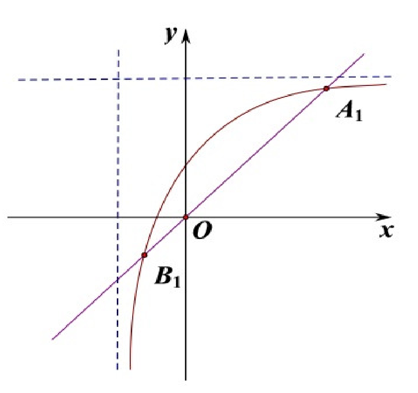
(2) When $br-c>0$, $A_1(\frac{q-p}{2\omega },\frac{q-p}{2\omega })$ is a positive equilibrium of system (9), $B_1(-\frac{p+q}{2\omega },-\frac{p+q}{2\omega })$ is a negative equilibrium of system (9) (see Figure 1).

Figure 1. The locations of the equilibria under the case $br-c>0$. x denotes the density of the population and y indicates the impact of distributed time delay.

x denotes the density of the population, y indicates the impact of distributed time delay. There are two solid lines on every sub-chart. The straight line is the equation: $\alpha x-\alpha y=0$, the curve is the equation: $x(r-\omega y)-\frac{cx}{b+x}=0$. The dotted lines in the Figures are asymptotes to the equation: $x(r-\omega y)-\frac{cx}{b+x}=0$. The intersections of two solid lines are shown in the following figure.

Theorem 1.

If $br-c>0$, the equilibrium $O(0,0)$ of system (9) is a saddle point. If $br-c>0$ and $\eta <0,$ the equilibrium $A_1$ of system (9) is globally asymptotically stable, where $\eta =(k-q)(q-p)-2\alpha (q+k)$.

Proof. 

When $br-c>0$, the Jacobi matrix of system (9) is

$$J=\left(\begin{array}{cc}\frac{\partial P}{\partial x}& \frac{\partial P}{\partial y}\\ \frac{\partial Q}{\partial x}& \frac{\partial Q}{\partial y}\end{array}\right)=\left(\begin{array}{cc}r-\omega y-\frac{bc}{{(b+x)}^2}& -\omega x\\ \alpha & -\alpha \end{array}\right).$$

(10)

At the equilibrium O, the Jacobi matrix of system (9) becomes

$$\begin{array}{c}{J|}_O=\left(\begin{array}{cc}r-\frac{c}{b}& 0\\ \alpha & -\alpha \end{array}\right),\hfill \end{array}$$

which allows us to obtain

$$\det \left(J{|}_O\right)=\frac{\alpha (c-br)}{b}.$$

Since $br-c>0$, then $\det \left(J{|}_O\right)<0$. Obviously, $O(0,0)$ is a saddle point.

At the equilibrium $A_1$, the Jacobi matrix of system (9) becomes

$$\begin{array}{c}{J|}_{A_1}=\left(\begin{array}{cc}r+\frac{p-q}{2}-\frac{4{\omega }^{2}bc}{{(q+k)}^2}& \frac{p-q}{2}\\ \alpha & -\alpha \end{array}\right).\hfill \end{array}$$

Then we get

$$\mathrm{tr}\left(J{|}_{A_1}\right)=r+\frac{p-q}{2}-\frac{4{\omega }^{2}bc}{{(q+k)}^2}-\alpha ,$$

$$\det \left(J{|}_{A_1}\right)=\alpha \left(-\omega b+q+\frac{4{\omega }^{2}bc}{{(q+k)}^2}\right).$$

Since we can also write $q^2=k^2-4\omega c$ and $p=\omega b-r$, it is easy for us to simplify $\det \left(J{|}_{A_1}\right)$ as follows

$$\det \left(J{|}_{A_1}\right)=\frac{\alpha q(q-p)}{q+k}.$$

Since $br-c>0$, we know that $q-p>0$ and $q+k>0$, then $\det \left(J{|}_{A_1}\right)>0$.

Next, we simplify $\mathrm{tr}\left(J{|}_{A_1}\right)$ as follows

$$\mathrm{tr}\left(J{|}_{A_1}\right)=\frac{(k-q)(q-p)-2\alpha (q+k)}{2(q+k)}.$$

Let

$$\eta =(k-q)(q-p)-2\alpha (q+k).$$

We have $\mathrm{tr}\left(J{|}_{A_1}\right)<0$ for $\eta <0$, $\mathrm{tr}\left(J{|}_{A_1}\right)>0$ as $\eta >0$, $\mathrm{tr}\left(J{|}_{A_1}\right)=0$ when $\eta =0$.

We discuss the situation of $\mathrm{tr}\left(J{|}_{A_1}\right)<0,$ i.e., $\eta <0$.

If $br-c>0$, then $\mathrm{tr}\left(J{|}_{A_1}\right)<0$, the positive equilibrium $A_1$ is locally stable in this case. Next, we are going to prove that there is no closed cycle in $\mathsf{\Omega }$. There is a unique positive equilibrium $A_1(\frac{q-p}{2\omega },\frac{q-p}{2\omega })$ in $\mathsf{\Omega }$, for convenience, we substitute $A_1(x_1,y_1)$ for $A_1(\frac{q-p}{2\omega },\frac{q-p}{2\omega })$. Suppose that there is a closed orbit $\mathsf{\Gamma }$ around $A_1$, which is, $x=x\left(t\right),y=y\left(t\right),-\infty <t<+\infty$, so there must exist a periodic T such that $x\left(T\right)=x\left(0\right),y\left(T\right)=y\left(0\right)$.

We calculate the index ${\gamma }_0$ of the closed orbit $\mathsf{\Gamma }$

$${\gamma }_0=\frac{1}{T}{\int }_0^T[P_x^{\prime }(x\left(t\right),y\left(t\right))+Q_y^{\prime }(x\left(t\right),y\left(t\right))]\mathrm{d}t,$$

where

$$P(x,y)=(r-\omega y-\frac{c}{b+x})x\mathrm{and}Q(x,y)=\alpha x-\alpha y.$$

We rewrite system (9) as follows

$$\left\{\begin{array}{c}(r-\omega y-\frac{c}{b+x})\mathrm{d}t=\frac{\mathrm{d}x}{x},\hfill \\ (\alpha x-\alpha y)\mathrm{d}t=\mathrm{d}y.\hfill \end{array}\right.$$

Integrating the two sides along the closed orbit $\mathsf{\Gamma }$, we get

$${\int }_0^T[r-\omega y\left(t\right)-\frac{c}{b+x\left(t\right)}]\mathrm{d}t={\int }_{x\left(0\right)}^{x\left(T\right)}\frac{\mathrm{d}x}{x}=ln\left|x\right|{\mid }_{x\left(0\right)}^{x\left(T\right)}=0,$$

$${\int }_0^T[\alpha x\left(t\right)-\alpha y\left(t\right)]\mathrm{d}t={\int }_{y\left(0\right)}^{y\left(T\right)}\mathrm{d}y=y{\mid }_{y\left(0\right)}^{y\left(T\right)}=0.$$

So we know that $\frac{1}{T}{\int }_0^{T}x\left(t\right)\mathrm{d}t$ and $\frac{1}{T}{\int }_0^{T}y\left(t\right)\mathrm{d}t$ also satisfy the following algebraic equation

$$\left\{\begin{array}{c}r-\omega y-\frac{c}{b+x}=0,\hfill \\ \alpha x-\alpha y=0.\hfill \end{array}\right.$$

Hence

$$\left\{\begin{array}{c}\frac{1}{T}{\int }_0^{T}x\left(t\right)\mathrm{d}t=x_1,\hfill \\ \frac{1}{T}{\int }_0^{T}y\left(t\right)\mathrm{d}t=y_1,\hfill \end{array}\right.$$

where $(x_1,y_1)$ is the coordinate of the equilibrium $A_1$. We obtain the index ${\gamma }_0$ of the closed orbit $\mathsf{\Gamma }$

$$\begin{array}{c}{\gamma }_0=\frac{1}{T}{\int }_0^T(r-\omega y-\frac{bc}{{(b+x)}^2}-\alpha )\mathrm{d}t\hfill \\ \phantom{{\gamma }_0}=\frac{1}{T}{\int }_0^T(\frac{cx}{{(b+x)}^2}-\alpha )\mathrm{d}t\hfill \\ \phantom{{\gamma }_0}=\frac{c{x}_1}{{(b+x_1)}^2}-\alpha .\hfill \end{array}$$

As $x_1=\frac{q-p}{2\omega }$, we have

$${\gamma }_0=\frac{(k-q)(q-p)-2\alpha (q+k)}{2(q+k)}<0.$$

The closed orbit $\mathsf{\Gamma }$ is stable as ${\gamma }_0<0$, which is contradicted by the fact that the equilibrium $A_1$ is asymptotically stable. Therefore, there is no closed orbit.

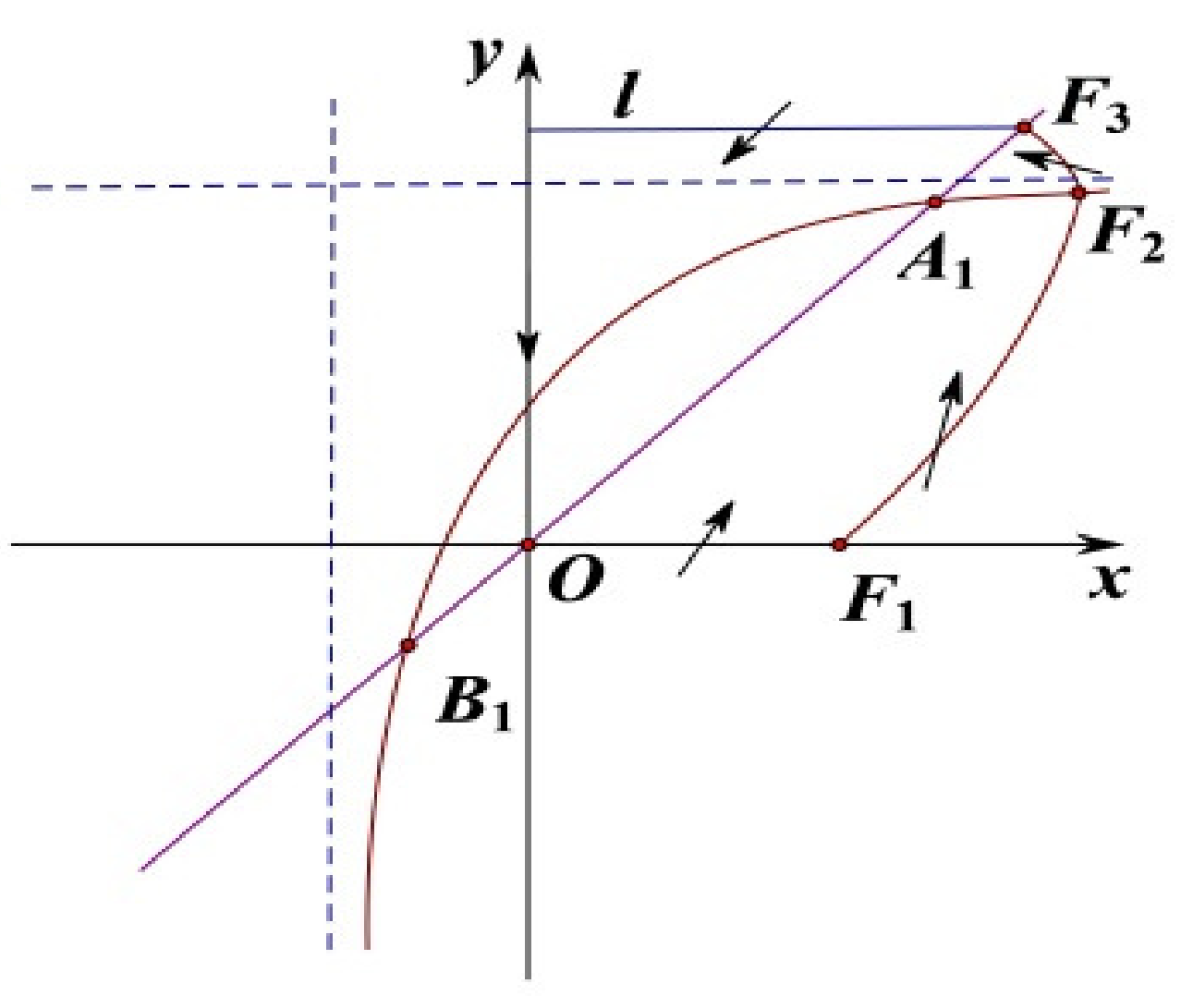
Now, we are going to prove that the solution of system (9) is eventually uniformly bounded (see Figure 2). Take a point $F_1$ on x-axis, draw the trajectory passing through the point $F_1$ of the following equation

$$\left\{\begin{array}{c}\frac{\mathrm{d}x}{\mathrm{d}t}=x(r-\omega y-\frac{c}{b+x}),\hfill \\ \frac{\mathrm{d}y}{\mathrm{d}t}=\frac{\alpha }{2}x-\frac{\alpha }{2}y,\hfill \end{array}\right.$$

and the trajectory intersects isoclinic line $r-\omega y-\frac{c}{b+x}=0$ at $F_2$. Comparing the direction of trajectory of system (9) with the tangent direction of trajectory $F_1{F}_2$ of the above system on $\stackrel{⌢}{F_1{F}_2}$ yields that

$$\frac{\alpha x-\alpha y}{x(r-\omega y-\frac{c}{b+x})}-\frac{\alpha x-\alpha y}{2x(r-\omega y-\frac{c}{b+x})}=\frac{\alpha x-\alpha y}{2x(r-\omega y-\frac{c}{b+x})}>0.$$

Figure 2. It shows that the solution of system (9) is uniformly bounded in $\mathsf{\Omega }$.

So the trajectory on $\stackrel{⌢}{F_1{F}_2}$ of system (9) goes through into the interior of $\stackrel{⌢}{F_1{F}_2}$ from the outer of $\stackrel{⌢}{F_1{F}_2}$ when the trajectory of system (9) intersects $\stackrel{⌢}{F_1{F}_2}$. Then draw the trajectory of the following equation

$$\left\{\begin{array}{c}\frac{\mathrm{d}x}{\mathrm{d}t}=x(r-\omega y-\frac{c}{b+x}),\hfill \\ \frac{\mathrm{d}y}{\mathrm{d}t}=\alpha x,\hfill \end{array}\right.$$

passing through the point $F_2$, and the trajectory will intersect isoclinic line $y=x$ at $F_3$. Comparing the direction of trajectory of system (9) with the tangent direction of trajectory $F_2{F}_3$ of above system on $\stackrel{⌢}{F_2{F}_3}$, we have

$$\frac{\alpha x-\alpha y}{x(r-\omega y-\frac{c}{b+x})}-\frac{\alpha x}{x(r-\omega y-\frac{c}{b+x})}=\frac{-\alpha y}{x(r-\omega y-\frac{c}{b+x})}>0.$$

So the trajectory on $\stackrel{⌢}{F_2{F}_3}$ of system (9) goes through into the interior of $\stackrel{⌢}{F_2{F}_3}$ from the outer of $\stackrel{⌢}{F_2{F}_3}$ when the trajectory of system (9) intersects $\stackrel{⌢}{F_2{F}_3}$. Then draw the line l from the point $F_3$, which is perpendicular to y-axis. The trajectory of system (9) goes through into the interior of l from the outer of l when the trajectory of system (9) intersects line l. Furthermore, y-axis is an isoclinic line, and the trajectory of system (9) goes through into the interior of x-axis from the outer of x-axis when intersects x-axis. According to the above analysis, the solution of system (9) is eventually uniformly bounded in $\mathsf{\Omega }$. In addition, there is no closed orbit in $\mathsf{\Omega }$. So the unique positive equilibrium $A_1(\frac{q-p}{2\omega },\frac{q-p}{2\omega })$ is globally asymptotically stable. □

Next, we discuss the case of $\mathrm{tr}\left(J{|}_{A_1}\right)=0,$ i.e., $\eta =0$.

We shift point $A_1(x_1,y_1)$ of system (9) to the origin and system (9) can be rewritten as

$$\left\{\begin{array}{c}\frac{\mathrm{d}x}{\mathrm{d}t}=\frac{(k-q)(q-p)}{2(k+q)}x+\frac{p-q}{2}y-\omega xy+\frac{2{\omega }^{2}b(k-q)}{{(k+q)}^2}{x}^2-\frac{4{\omega }^{3}b(k-q)}{{(k+q)}^3}{x}^3+{\left[x\right]}_4,\hfill \\ \frac{\mathrm{d}y}{\mathrm{d}t}=\alpha x-\alpha y,\hfill \end{array}\right.$$

(11)

where ${\left[x\right]}_4$ is a ${\mathrm{C}}^{\infty }$ function of at least fourth order about x. In this case, $\mathrm{tr}\left(J{|}_{A_1}\right)=0$, that is $\eta =0$, then ${J|}_{A_1}$ becomes

$$\begin{array}{c}{J|}_{A_1^{{}^{\prime }}}=\left(\begin{array}{cc}\alpha & \frac{p-q}{2}\\ \alpha & -\alpha \end{array}\right).\hfill \end{array}$$

We can obtain $n\triangleq \sqrt{\det \left(J{|}_{A_1^{{}^{\prime }}}\right)}=\sqrt{-{\alpha }^2-\alpha \frac{p-q}{2}}>0$ by $\eta =0$. So we can know that the eigenvalues of ${J|}_{A_1^{{}^{\prime }}}$ are ${\lambda }_1=ni$ and ${\lambda }_2=-ni$ (i is the complex unit, similarly hereinafter) by simple calculation. Taking non-singular transformations $x=\frac{\overline{x}}{\alpha }-\frac{\overline{y}}{n}$ and $y=-\frac{\overline{y}}{n}$, and also denoting $\overline{x},\overline{y}$ by $x,y$, respectively, system (11) becomes

$$\left\{\begin{array}{c}\frac{\mathrm{d}x}{\mathrm{d}t}=-ny+f(x,y),\hfill \\ \frac{\mathrm{d}y}{\mathrm{d}t}=nx+g(x,y),\hfill \end{array}\right.$$

where

$$\begin{array}{cc}\hfill f(x,y)& =-\frac{\omega {(k+q)}^2-4{\omega }^{2}b(k-q)}{n{(k+q)}^2}xy+\frac{2{\omega }^{2}b(k-q)}{\alpha {(k+q)}^2}{x}^2+\frac{2\alpha {\omega }^{2}b(k-q)-\alpha \omega {(k+q)}^2}{n^2{(k+q)}^2}{y}^2\hfill \\ & -\frac{4{\omega }^{3}b(k-q)}{{\alpha }^2{(k+q)}^3}{x}^3-\frac{12{\omega }^{3}b(k-q)}{\alpha n{(k+q)}^3}{x}^{2}y-\frac{12{\omega }^{3}b(k-q)}{n^2{(k+q)}^3}x{y}^2-\frac{4\alpha {\omega }^{3}b(k-q)}{n^3{(k+q)}^3}{y}^3\hfill \\ & +{[x,y]}_4,\hfill \\ \hfill g(x,y)& =0,\hfill \end{array}$$

where ${[x,y]}_4$ is a ${\mathrm{C}}^{\infty }$ function of at least fourth order about x and y. $f(x,y)$ and $g(x,y)$ are ${\mathrm{C}}^{\infty }$ functions and satisfy $f(0,0)=g(0,0)=0$.

Using the formula for the Lyapunov number of Andronov et al. [30], we have the first Lyapunov number ${\alpha }_1$ of the equilibrium $A_1$ of system (9) as follows

$$\begin{array}{cc}\hfill {\alpha }_1& =\{\frac{1}{16}(f_{xxx}+f_{xyy}+g_{xxy}+g_{yyy})+\frac{1}{16n}(f_{xy}(f_{xx}+f_{yy})\hfill \\ & -g_{xy}(g_{xx}+g_{yy})-f_{xx}{g}_{xx}+f_{yy}{g}_{yy}\left)\right\}{|}_{x=0,y=0}\hfill \\ & =\frac{1}{8}[-\frac{12{\omega }^{3}b(k-q)}{{\alpha }^2{(k+q)}^3}-\frac{12{\omega }^{3}b(k-q)}{n^2{(k+q)}^3}-\frac{\omega {(k+q)}^2-4{\omega }^{2}b(k-q)}{n{(k+q)}^2}·\frac{2{\omega }^{2}b(k-q)}{\alpha n{(k+q)}^2}\hfill \\ & -\frac{\omega {(k+q)}^2-4{\omega }^{2}b(k-q)}{n{(k+q)}^2}·\frac{2\alpha {\omega }^{2}b(k-q)-\alpha \omega {(k+q)}^2}{n^3{(k+q)}^2}]\hfill \\ & =\frac{{\omega }^2}{8{\alpha }^2{n}^4{(k+q)}^4}[-12\omega b{n}^4(k^2-q^2)-12\omega b{\alpha }^2{n}^2(k^2-q^2)-2\omega b\alpha n^2{(k+q)}^2(k-q)\hfill \\ & +8{\omega }^2{b}^2\alpha n^2{(k-q)}^2-6\omega b{\alpha }^3{(k+q)}^2(k-q)+{\alpha }^3{(k+q)}^4+8{\omega }^2{b}^2{\alpha }^3{(k-q)}^2]\hfill \\ & =-\frac{{\omega }^2(q-p)}{8\alpha n^4{(k+q)}^3}\left[2\omega b{n}^2(k-q)+{\alpha }^2(q+k)(2\omega b+p-q)\right].\hfill \end{array}$$

If

$$2\omega b{n}^2(k-q)+{\alpha }^2(q+k)(2\omega b+p-q)>0$$

(12)

holds, it follows that ${\alpha }_1<0$, where $n=\sqrt{-{\alpha }^2-\alpha \frac{p-q}{2}}.$ So we obtain the following theorem:

Theorem 2.

If $br-c>0$ and condition (12) holds, a supercritical Hopf bifurcation occurs near $A_1$ when η passes through 0, where $\eta =(k-q)(q-p)-2\alpha (q+k)$.

Then, we discuss the case of $\mathrm{tr}\left(J{|}_{A_1}\right)>0,$ i.e., $\eta >0$.

When $br-c>0$ and $\eta >0$, the positive equilibrium $A_1$ is an unstable focus or node. Given what has been proved before, it is not difficult to obtain that the solution of system (9) is also uniformly bounded in $\mathsf{\Omega }$. Since the unique positive equilibrium $A_1$ is unstable, we can obtain that there exists at least one limit cycle which is stable in region $\mathsf{\Omega }$ by Poincaré-Bendixson Theorem.

Particularly, we have known that a Hopf bifurcation occurs when $br-c>0$ and condition (12) holds. That is to say, the equilibrium $A_1$ is not a true center. The derivative of system (9) at the point $A_1$ is denoted as $A\left(\eta \right)$. We can get the eigenvalues of $A\left(0\right)$ are $\pm ni$, i.e.,

$$\mathrm{Tr}A\left(0\right)=0,\det A\left(0\right)>0.$$

We also define the matrix $B\left(\eta \right)$ which satisfies

$$A\left(\eta \right)=A\left(0\right)+\eta B\left(\eta \right).$$

We obtain that $\mathrm{Tr}B\left(0\right)\ne 0$. Using the Friedrich Theorem of Hopf bifurcation, we get the truth that there exists a unique stable limit cycle near $A_1$ when $br-c>0,\eta >0$ and condition (12) holds. So we get the following Theorem:

Theorem 3.

If $br-c>0$ and $\eta >0$, there exists at least one limit cycle which is stable in Ω. Particularly, there exists a unique stable limit cycle near $A_1$ when $br-c>0,\eta >0$ and condition (12) holds, where $\eta =(k-q)(q-p)-2\alpha (q+k)$.

4. The Existence and Stability of the Equilibria for $\mathit{br}-\mathit{c}<\mathbf{0}$

Let us consider the existence and stability of the equilibria for the case $br-c<0$.

(1) $O(0,0)$ is clearly an equilibrium of system (9).

(2) When $br-c<0,r-\omega b>0$ and $q^2>0$, $A_2(-\frac{p+q}{2\omega },-\frac{p+q}{2\omega })$ and $A_3(\frac{q-p}{2\omega },\frac{q-p}{2\omega })$ are positive equilibria of system (9), where $\frac{q-p}{2\omega }>-\frac{p+q}{2\omega }>0$ (see Figure 3I).

Figure 3. Figure (I–V) show the locations of the equilibria under the case $br-c<0$. x denotes the density of the population and y indicates the impact of distributed time delay. Figure (I) shows the locations of the equilibra in the case $br-c<0, r-\omega b>0$ and $q^2>0$; The conditions for Figure (II) are $br-c<0, r-\omega b>0$ and $q^2=0$; $br-c<0, r-\omega b<0$ and $q^2>0$ correspond to Figure (II); $br-c<0, r-\omega b<0$ and $q^2=0$ are the conditions of Figure (IV); Figure (V) represents the equilibrium of the system under the case $br-c<0$ and $r-\omega b=0$.

(3) When $br-c<0,r-\omega b>0$ and $q^2=0$, $A_4(-\frac{p}{2\omega },-\frac{p}{2\omega })$ is a positive equilibrium of system (9) (see Figure 3II).

(4) When $br-c<0,r-\omega b<0$ and $q^2>0$, $B_2(-\frac{p+q}{2\omega },-\frac{p+q}{2\omega })$ and $B_3(\frac{q-p}{2\omega },\frac{q-p}{2\omega })$ are negative equilibria of system (9), where $-\frac{p+q}{2\omega }<\frac{q-p}{2\omega }<0$. Considering the practical significance, this case will not be discussed (see Figure 3III).

(5) When $br-c<0,r-\omega b<0$ and $q^2=0$, $B_4(-\frac{p}{2\omega },-\frac{p}{2\omega })$ is a negative equilibrium of system (9), this case will not be discussed (see Figure 3IV).

(6) When $br-c<0$ and $r-\omega b=0$, system (9) has no more equilibrium except $O(0,0)$ (see Figure 3V).

Theorem 4.

If $br-c<0$, the equilibrium $O(0,0)$ of system (9) is locally stable. More precisely, If $br-c<0$ and $r-\omega b=0$, the positive equilibrium $O(0,0)$ of system (9) is globally asymptotically stable. If $br-c<0,r-\omega b>0$ and $q^2>0$, the positive equilibrium $A_2$ of system (9) is a saddle point. If $br-c<0,r-\omega b>0,q^2>0$ and $\beta <0$, the positive equilibrium $A_3$ of system (9) is locally stable. If $br-c<0,r-\omega b>0,q^2>0$ and $\beta >0$, the positive equilibrium $A_3$ of system (9) is unstable, where $\beta =(k-q)(q-p)-2\alpha (q+k)$.

Proof. 

Firstly, we analyze the stability of the equilibrium $O(0,0)$ of system (9). Through the preceding discussion, we have

$$\det \left(J{|}_O\right)=\frac{-\alpha (br-c)}{b},\mathrm{tr}\left(J{|}_O\right)=\frac{br-c-\alpha b}{b}.$$

When $br-c<0$, it is easy to get $\det \left(J{|}_O\right)>0$ and $\mathrm{tr}\left(J{|}_O\right)<0$. So the equilibrium O is locally stable. Particularly, when $br-c<0$ and $r-\omega b=0$, System (9) has only one equilibrium $O(0,0)$. According to what we have proved before, the solution of system (9) is eventually uniformly bounded in $\mathsf{\Omega }$ under this case. Since $x=0$ is the isoclinic line, it is not possible in the whole plane to have a closed orbit which surrounds the equilibrium O. If system (9) has a limit cycle which exists in first quadrant, it must contain the equilibrium $A_4$ in the limit cycle. However, under this circumstance, system (9) has no other equilibria except $O(0,0)$, so we have the conclusion that system (9) has no limit cycle when $br-c<0$ and $r-\omega b=0$. Like the proof of Theorem 1, we know that equilibrium O is globally asymptotically stable when $br-c<0$ and $r-\omega b=0$; that is, all trajectories of the solution tend to equilibrium O if $br-c<0$ and $r-\omega b=0$.

Secondly, we discuss the stability of the positive equilibrium $A_2$. We substitute $A_2(-\frac{p+q}{2\omega },-\frac{p+q}{2\omega })$ into (10) to get

$$\begin{array}{c}{J|}_{A_2}=\left(\begin{array}{cc}r+\frac{p+q}{2}-\frac{4{\omega }^{2}bc}{{(q-k)}^2}& \frac{p+q}{2}\\ \alpha & -\alpha \end{array}\right),\hfill \end{array}$$

and we have

$$\det \left(J{|}_{A_2}\right)=-\omega b+q+\frac{4{\omega }^{2}bc}{{(q-k)}^2},$$

$$\mathrm{tr}\left(J{|}_{A_2}\right)=r+\frac{p+q}{2}-\frac{4{\omega }^{2}bc}{{(q-k)}^2}-\alpha .$$

It follows from $q^2=k^2-4\omega c$ and $p=\omega b-r$ that $\det \left(J{|}_{A_2}\right)$ becomes

$$\det \left(J{|}_{A_2}\right)=\frac{-\alpha q(p+q)}{q-k}.$$

Since $p+q<0$ and $q-k<0,$ we get

$$\det \left(J{|}_{A_2}\right)<0.$$

Apparently, when $br-c<0,r-\omega b>0$ and $q^2>0,$ the positive equilibrium $A_2$ is a saddle point.

Finally, we analyze the stability of the positive equilibrium $A_3$. We substitute $A_3(\frac{q-p}{2\omega },\frac{q-p}{2\omega })$ into (10) to get

$$\begin{array}{c}{J|}_{A_3}=\left(\begin{array}{cc}r+\frac{p-q}{2}-\frac{4{\omega }^{2}bc}{{(q+k)}^2}& \frac{p-q}{2}\\ \alpha & -\alpha \end{array}\right),\hfill \end{array}$$

which yields

$$\det \left(J{|}_{A_3}\right)=\alpha (-\omega b+q+\frac{4{\omega }^{2}bc}{{(q+k)}^2}),$$

$$\mathrm{tr}\left(J{|}_{A_3}\right)=r+\frac{p-q}{2}-\frac{4{\omega }^{2}bc}{{(q+k)}^2}-\alpha .$$

Through simplification, we obtain

$$\det \left(J{|}_{A_3}\right)=\frac{\alpha q(q-p)}{q+k}.$$

It follows from the inequalities $br-c<0,r-\omega b>0,q^2>0,p-q<0$ and $q+k>0$ that $\det \left(J{|}_{A_3}\right)>0$. We also simplify $\mathrm{tr}\left(J{|}_{A_3}\right)$ to get

$$\mathrm{tr}\left(J{|}_{A_3}\right)=\frac{(k-q)(q-p)-2\alpha (q+k)}{2(q+k)}.$$

Let

$$\beta =(k-q)(q-p)-2\alpha (q+k).$$

Suppose that $\beta <0,$ then $\mathrm{tr}\left(J{|}_{A_3}\right)<0$, which means the positive equilibrium $A_3$ is locally stable. Under this circumstance, there are three equilibria for system (9). Therefore, we only consider the local situation of system (9). Since $O(0,0)$ is locally stable, and $A_2$ is always a saddle point, and $A_3$ is locally asymptotically stable, the trajectory of the solution tends to the equilibrium point $A_3$ when the initial value is selected in the attraction domain of equilibrium point $A_3$, or the trajectory of the solution tends to the equilibrium point O when the initial value is selected in the attraction domain of equilibrium point O.

Suppose that $\beta =0,$ then $\mathrm{tr}\left(J{|}_{A_3}\right)=0$, which means $A_3$ is a center-type singular point. Under this circumstance, the trajectory of the solution tends to the equilibrium point O or forms a closed trajectory near $A_3$. In this case, system (9) admits the probability that a Hopf bifurcation occurs near $A_3$. Since the form of $A_3$ is the same with $A_1$, we use the result of Theorem 2 to obtain the first Lyapunov number ${\alpha }_2$ of $A_3$:

$${\alpha }_2=-\frac{{\omega }^2(q-p)}{8\alpha n^4{(k+q)}^3}\left[2\omega b{n}^2(k-q)+{\alpha }^2(q+k)(2\omega b+p-q)\right].$$

If

$$2\omega b{n}^2(k-q)+{\alpha }^2(q+k)(2\omega b+p-q)>0$$

(13)

holds, it follows that ${\alpha }_2<0$. So we get that a supercritical Hopf bifurcation occurs near $A_3$.

Suppose that $\beta >0,$ then $\mathrm{tr}\left(J{|}_{A_3}\right)>0$, which means the positive equilibrium $A_3$ is unstable. Under this circumstance, if $O(0,0)$ is locally stable, and $A_2$ is always a saddle point, and $A_3$ is unstable, then, there is a stable limit cycle generated by Hopf bifurcation in the neighborhood of $A_3$ when $0<\beta \ll 1$. All trajectories of system (9) will be far away from $A_3$ and tend to O. □

Next, we analyze the situation that $A_2$ and $A_3$ are merged into a single equilibrium point $A_4$. We first give the Theorem 5 and then prove it.

Theorem 5.

If $br-c<0,r-\omega b>0$ and $q^2=0$, the unique positive equilibrium $A_4$ is degenerate, and system (9) has no limit cycle in Ω. The equilibrium O is globally asymptotically stable. More precisely, if $br-c<0,r-\omega b>0,q^2=0$ and $r-\omega b-2\alpha \ne 0$, the equilibrium $A_4$ is a saddle node. If $br-c<0,r-\omega b>0,q^2=0$ and $r-\omega b-2\alpha =0$, the equilibrium $A_4$ is a degenerate critical point.

Proof. 

We substitute $A_4(-\frac{p}{2\omega },-\frac{p}{2\omega })$ into (10) to obtain

$$\begin{array}{c}{J|}_{A_4}=\left(\begin{array}{cc}r+\frac{p}{2}-\frac{4{\omega }^{2}bc}{k^2}& \frac{p}{2}\\ \alpha & -\alpha \end{array}\right),\hfill \end{array}$$

(14)

which yields

$$\det \left(J{|}_{A_4}\right)=-\alpha (r+\frac{p}{2}-\frac{4{\omega }^{2}bc}{k^2})-\frac{\alpha p}{2}.$$

where $k=r+\omega b$ and $p=\omega b-r$, it is easy to get $\det \left(J{|}_{A_4}\right)=0$. It can easily be shown that this equilibrium point is a higher order singular point. Now we do this work. We shift this point $A_4(x_4,y_4)$ of system (9) to the origin, then, system (9) can be written as

$$\left\{\begin{array}{c}\frac{\mathrm{d}x}{\mathrm{d}t}=\frac{r-\omega b}{2}x-\frac{r-\omega b}{2}y-\omega xy+\frac{2{\omega }^{2}b}{r+\omega b}{x}^2-{\left[x\right]}_3,\hfill \\ \frac{\mathrm{d}y}{\mathrm{d}t}=\alpha x-\alpha y,\hfill \end{array}\right.$$

(15)

where ${\left[x\right]}_3$ is a ${\mathrm{C}}^{\infty }$ function of at least third order about x.

When $r-\omega b-2\alpha \ne 0$, (14) changes into

$$\begin{array}{c}{J|}_{A_4}=\left(\begin{array}{cc}\frac{r-\omega b}{2}& -\frac{r-\omega b}{2}\\ \alpha & -\alpha \end{array}\right).\hfill \end{array}$$

Then the eigenvalues of ${J|}_{A_4}$ are ${\lambda }_1=0$ and ${\lambda }_2=\frac{r-\omega b-2\alpha }{2}$. At this time, $A_4$ is a codimension 1 singular point. Using $x=\overline{x}+\overline{y}$, $y=\overline{x}+\frac{2\alpha }{r-\omega b}\overline{y}$ and $\mathrm{d}t=\frac{2}{r-\omega b-2\alpha }\mathrm{d}\tau$, we also denote $\overline{x},\overline{y}$ and $\tau$ by $x,y$ and t, respectively. System (15) becomes

$$\left\{\begin{array}{c}\frac{\mathrm{d}x}{\mathrm{d}t}=\frac{4\alpha \omega (r-\omega b)}{(r+\omega b){(r-\omega b-2\alpha )}^2}{x}^2+\frac{4\alpha \omega {(r-\omega b)}^2+8{\alpha }^2\omega (r+\omega b)}{(r+\omega b)(r-\omega b){(r-\omega b-2\alpha )}^2}xy+\frac{8\alpha {\omega }^{2}b(\omega b-r)+8{\alpha }^2\omega (r+\omega b)}{(r+\omega b)(r-\omega b){(r-\omega b-2\alpha )}^2}{y}^2-{\left[x\right]}_3,\hfill \\ \frac{\mathrm{d}y}{\mathrm{d}t}=y-\frac{2\omega {(r-\omega b)}^2}{(r+\omega b){(r-\omega b-2\alpha )}^2}{x}^2-\frac{2\omega {(r-\omega b)}^2+4\alpha \omega (r+\omega b)}{(r+\omega b){(r-\omega b-2\alpha )}^2}xy+\frac{4{\omega }^{2}b(r-\omega b)-4\alpha \omega (r+\omega b)}{(r+\omega b){(r-\omega b-2\alpha )}^2}{y}^2-{\left[x\right]}_3.\hfill \end{array}\right.$$

Apply $\frac{\mathrm{d}y}{\mathrm{d}t}=0$ to get

$$\begin{array}{cc}\hfill y=& \frac{2\omega {(r-\omega b)}^2}{(r+\omega b){(r-\omega b-2\alpha )}^2}{x}^2+\frac{2\omega {(r-\omega b)}^2+4\alpha \omega (r+\omega b)}{(r+\omega b){(r-\omega b-2\alpha )}^2}xy\hfill \\ & -\frac{4{\omega }^{2}b(r-\omega b)-4\alpha \omega (r+\omega b)}{(r+\omega b){(r-\omega b-2\alpha )}^2}{y}^2+{\left[x\right]}_3.\hfill \end{array}$$

We take the above equality into $\frac{\mathrm{d}x}{\mathrm{d}t}$ and obtain

$$\frac{\mathrm{d}x}{\mathrm{d}t}=\frac{4\alpha \omega (r-\omega b)}{(r+\omega b){(r-\omega b-2\alpha )}^2}{x}^2+{[x,y]}_3,$$

where ${[x,y]}_3$ is a ${\mathrm{C}}^{\infty }$ function of at least third order about x and y. It follows that the right side of the above equality is a polynomial about x and y, and the order of it is at least two.

By Theorem 7.1 in Chapter 2 of Zhang et al. [31], we know that $A_4$ is a saddle node.

When $r-\omega b-2\alpha =0$, (14) changes into

$$\begin{array}{c}{J|}_{A_4}=\left(\begin{array}{cc}\alpha & -\alpha \\ \alpha & -\alpha \end{array}\right).\hfill \end{array}$$

Then the eigenvalues of ${J|}_{A_4}$ are ${\lambda }_1=0$ and ${\lambda }_2=0$. That is, $A_4$ is a codimension 1 singular point. System (15) becomes

$$\left\{\begin{array}{c}\frac{\mathrm{d}x}{\mathrm{d}t}=\alpha x-\alpha y-\omega xy+\frac{2{\omega }^{2}b}{r+\omega b}{x}^2-{\left[x\right]}_3,\hfill \\ \frac{\mathrm{d}y}{\mathrm{d}t}=\alpha x-\alpha y.\hfill \end{array}\right.$$

(16)

Taking the non-singular transformations $x=\overline{x}+\overline{y}$, $y=\overline{x}-\overline{y}$ and $\mathrm{d}t=\frac{1}{2\alpha }\mathrm{d}\tau$, we also denote $\overline{x},\overline{y}$ and $\tau$ by $x,y$ and t, respectively. System (16) becomes

$$\left\{\begin{array}{c}\frac{\mathrm{d}x}{\mathrm{d}t}=y-\frac{\omega }{2(r+\omega b)}{x}^2+\frac{\omega }{4\alpha }{y}^2-{\left[x\right]}_3\triangleq y+P_2(x,y),\hfill \\ \frac{\mathrm{d}y}{\mathrm{d}t}=-\frac{\omega }{2(r+\omega b)}{x}^2+\frac{\omega }{4\alpha }{y}^2-{\left[x\right]}_3\triangleq Q_2(x,y).\hfill \end{array}\right.$$

(17)

By a one-to-one transformation in a sufficiently small neighborhood of the origin

$$x\to x,y+P_2(x,y)\to y,$$

system (17) becomes

$$\left\{\begin{array}{c}\frac{\mathrm{d}x}{\mathrm{d}t}=y,\hfill \\ \frac{\mathrm{d}y}{\mathrm{d}t}={\tilde{Q}}_2(x,y).\hfill \end{array}\right.$$

(18)

We still denote ${\tilde{Q}}_2(x,y)$ by $Q_2(x,y)$ with terms of order no less than two. We write

$$Q_2(x,y)=-\frac{\omega }{2(r+\omega b)}{x}^2(1+h\left(x\right))+(-\frac{\omega }{r+\omega b})xy(1+g\left(x\right))+y^{2}f(x,y),$$

where $h\left(x\right),g\left(x\right)$ and $f(x,y)$ are analytic functions, moreover, $h\left(0\right)=g\left(0\right)=0$. Hence the origin of system (18) is a double singularity.

By Theorem 7.3 in Chapter 2 and its Corollary of Zhang et al. [31], we find that the origin of system (17) is a degenerate critical point. That is, the equilibrium point $A_4$ of system (9) is a degenerate critical point.

According to what we have proved before, the solution of system (9) is eventually uniformly bounded in $\mathsf{\Omega }$ under this case. Since $x=0$ is the isoclinic line, it is not possible in the whole plane to have a closed orbit which surrounds the equilibrium O. If system (9) has a limit cycle which exists in first quadrant, there must contain the equilibrium $A_4$ in the limit cycle, and the index of it must be one. However, the index of equilibrium $A_4$ is zero whether it is a saddle node or a degenerate critical point, so we have the conclusion that system (9) has no limit cycle when $br-c<0,r-\omega b>0,q^2=0$. The same to the proof of Theorem 1, we know that equilibrium O is globally asymptotically stable when $br-c<0,r-\omega b>0$ and $q^2=0$. That is, all trajectories of the solution tend to equilibrium O when $br-c<0,r-\omega b>0$ and $q^2=0$. □

5. The Existence and Stability of the Equilibria for $\mathit{br}-\mathit{c}=\mathbf{0}$

Let us consider the existence and stability of the equilibria for the case $br-c=0$.

(1) $O(0,0)$ is clearly an equilibrium of system (9).

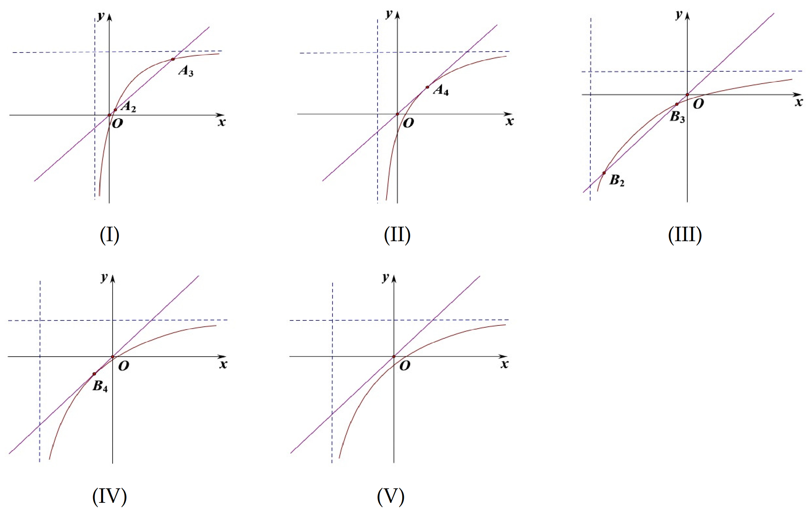
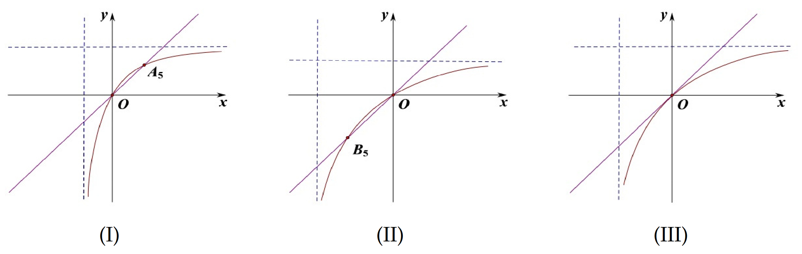
(2) When $br-c=0$ and $r-\omega b>0$, $A_5(\frac{r-\omega b}{\omega },\frac{r-\omega b}{\omega })$ is a positive equilibrium of system (9), where $\frac{r-\omega b}{\omega }>0$ (see Figure 4I).

Figure 4. Figure (I–III) show the locations of the equilibria under the case $br-c=0$, respectively. x denotes the density of the population. y indicates the impact of distributed time delay. Figure (I) corresponds to the case $br-c=0$ and $r-\omega b>0$; Fiure (II) shows the case $br-c=0$ and $r-\omega b<0$ and Figure (III) corresponds to the case $br-c=0$ and $r-\omega b=0$.

(3) When $br-c=0$ and $r-\omega b<0$, $B_5(-\frac{p+q}{2\omega },-\frac{p+q}{2\omega })$ is a negative equilibrium of system (9). This case will not be discussed (see Figure 4II).

(4) When $br-c=0$ and $r-\omega b=0$, system (9) has no more equilibria except $O(0,0)$ (see Figure 4III).

Theorem 6.

If $br-c=0$ and $r-\omega b=0,$ the equilibrium $O(0,0)$ of system (9) is an unstable node, and system (9) has a singular line. If $br-c=0$ and $r-\omega b\ne 0,$ the equilibrium $O(0,0)$ is a saddle node.

Proof. 

Firstly, we analyze the stability of the equilibrium $O(0,0)$ of system (9). We take $O(0,0)$ into (10) and get

$$\begin{array}{c}{J|}_O=\left(\begin{array}{cc}r-\frac{c}{b}& 0\\ 1& -1\end{array}\right),\hfill \end{array}$$

and

$$\det \left(J{|}_O\right)=\frac{c-br}{b}.$$

When $br-c=0$, we get $\det \left(J{|}_O\right)=0$. It can easily be shown that the equilibrium O is a higher order singular point. We change (9) into (19).

$$\left\{\begin{array}{c}\frac{\mathrm{d}x}{\mathrm{d}t}=-\omega xy+\frac{c}{b^2}{x}^2-\frac{c}{b^3}{x}^3+\frac{c}{b^4}{x}^4-{\left[x\right]}_5,\hfill \\ \frac{\mathrm{d}y}{\mathrm{d}t}=\alpha x-\alpha y.\hfill \end{array}\right.$$

(19)

Performing the nonsingular transformations $x=\overline{x}$, $y=\overline{x}-\overline{y}$ and $\mathrm{d}t=-\frac{1}{\alpha }\mathrm{d}\tau$, we still denote $\overline{x},\overline{y}$ and $\tau$ by $x,y$ and t, and (19) becomes

$$\left\{\begin{array}{c}\frac{\mathrm{d}x}{\mathrm{d}t}=(\frac{\omega }{\alpha }-\frac{c}{\alpha b^2})x^2-\frac{\omega }{\alpha }xy+\frac{c}{\alpha b^3}{x}^3-\frac{c}{\alpha b^4}{x}^4+{\left[x\right]}_5,\hfill \\ \frac{\mathrm{d}y}{\mathrm{d}t}=y+(\frac{\omega }{\alpha }-\frac{c}{\alpha b^2})x^2-\frac{\omega }{\alpha }xy+\frac{c}{\alpha b^3}{x}^3-\frac{c}{\alpha b^4}{x}^4+{\left[x\right]}_5.\hfill \end{array}\right.$$

(20)

When $\frac{\omega }{\alpha }-\frac{c}{\alpha b^2}=0$, i.e., $r-\omega b=0$, the positive equilibrium $A_5$ does not exist under this condition, that is, the equilibrium O is a triple singularity (20) becomes

$$\left\{\begin{array}{c}\frac{\mathrm{d}x}{\mathrm{d}t}=-\frac{\omega }{\alpha }xy+\frac{c}{\alpha b^3}{x}^3-\frac{c}{\alpha b^4}{x}^4+{\left[x\right]}_5\triangleq {\mathsf{\Phi }}_1(x,y),\hfill \\ \frac{\mathrm{d}y}{\mathrm{d}t}=y-\frac{\omega }{\alpha }xy+\frac{c}{\alpha b^3}{x}^3-\frac{c}{\alpha b^4}{x}^4+{\left[x\right]}_5\triangleq y+{\mathsf{\Psi }}_1(x,y).\hfill \end{array}\right.$$

Let $y+{\mathsf{\Psi }}_1(x,y)=0$, then

$$y=\frac{1}{1-\frac{\omega }{\alpha }x}(-\frac{c}{\alpha b^3}{x}^3+\frac{c}{\alpha b^4}{x}^4-{\left[x\right]}_5),$$

by Taylor expansion at $x=0$, we have

$$y=-\frac{c}{\alpha b^3}{x}^3+(\frac{c}{\alpha b^4}-\frac{c\omega }{{\alpha }^2{b}^3})x^4+{\left[x\right]}_5.$$

After some calculations, we have

$${\mathsf{\Phi }}_1(x,y)=\frac{c}{\alpha b^3}{x}^3+{\left[x\right]}_4.$$

By Theorem 7.1 in Chapter 2 of Zhang et al. [31], we know that O is an unstable node.

According to what we have proved before, the solution of system (9) is eventually uniformly bounded in $\mathsf{\Omega }$ under this case. Since $x=0$ is the isoclinic line, it is not possible in the whole plane to have a closed orbit which surrounds the equilibrium O. In addition, if the closed orbit exists in some quadrant, then there must be an equilibrium in the closed orbit. So we have the conclusion that there is no closed orbit in the whole plane when $br-c=0$ and $r-\omega b=0$. Meanwhile, the linear system of system (19) is as follows

$$\left\{\begin{array}{c}\frac{\mathrm{d}x}{\mathrm{d}t}=0,\hfill \\ \frac{\mathrm{d}y}{\mathrm{d}t}=\alpha x-\alpha y,\hfill \end{array}\right.$$

and ${\alpha }^2+{(-\alpha )}^2=2{\alpha }^2\ne 0$. It follows that system (19) has a singular line $\alpha x-\alpha y=0$, i.e., $y=x$ when $br-c=0$ and $r-\omega b=0$. Then all the trajectories tend to the singular line $y=x$.

When $\frac{\omega }{\alpha }-\frac{c}{\alpha b^2}\ne 0$, i.e., $r-\omega b\ne 0$, the positive equilibrium $A_5$ exists if $r-\omega b>0$, and the negative equilibrium $B_5$ exists if $r-\omega b<0$, that is, the equilibrium O is a double singularity. We rewrite (20) into the following equation

$$\left\{\begin{array}{c}\frac{\mathrm{d}x}{\mathrm{d}t}=(\frac{\omega }{\alpha }-\frac{c}{\alpha b^2})x^2-\frac{\omega }{\alpha }xy+\frac{c}{\alpha b^3}{x}^3-\frac{c}{\alpha b^4}{x}^4+{\left[x\right]}_5\triangleq {\mathsf{\Phi }}_2(x,y),\hfill \\ \frac{\mathrm{d}y}{\mathrm{d}t}=y+(\frac{\omega }{\alpha }-\frac{c}{\alpha b^2})x^2-\frac{\omega }{\alpha }xy+\frac{c}{\alpha b^3}{x}^3-\frac{c}{\alpha b^4}{x}^4+{\left[x\right]}_5\triangleq y+{\mathsf{\Psi }}_2(x,y).\hfill \end{array}\right.$$

Let $y+{\mathsf{\Psi }}_2(x,y)=0$, then

$$y=(\frac{c}{\alpha b^2}-\frac{\omega }{\alpha })x^2+{\left[x\right]}_3.$$

By some calculations, we derive

$${\mathsf{\Phi }}_2(x,y)=(\frac{\omega }{\alpha }-\frac{c}{\alpha b^2})x^2+{\left[x\right]}_3.$$

By Theorem 7.1 in Chapter 2 of [31], we know that O is a saddle node. □

Next, we are going to analyze the stability of the equilibrium $A_5$. Obviously, the equilibrium O as a saddle node simultaneously exists with the equilibrium $A_5$ when $br-c=0$ and $r-\omega b>0$. We first give the Theorem 7 and then prove it.

Theorem 7.

If $br-c=0,r-\omega b>0$ and $\xi <0$, the unique positive equilibrium point $A_5$ is locally stable. If $br-c=0,r-\omega b>0$ and $\xi >0$, the unique positive equilibrium $A_5$ is unstable and there exists at least one limit cycle in a small neighborhood of $A_5$.

Proof. 

We substitute $A_5(\frac{r-\omega b}{\omega },\frac{r-\omega b}{\omega })$ into (10) to derive

$$\begin{array}{c}{J|}_{A_5}=\left(\begin{array}{cc}\frac{\omega b(r-\omega b)}{r}& \omega b-r\\ \alpha & -\alpha \end{array}\right),\hfill \end{array}$$

which yields

$$\det \left(J{|}_{A_5}\right)=\frac{\alpha {(\omega b-r)}^2}{r},$$

$$\mathrm{tr}\left(J{|}_{A_5}\right)=\frac{\omega b(r-\omega b)-\alpha r}{r}.$$

It follows from the inequality $r-\omega b>0$ that $\det \left(J{|}_{A_5}\right)>0$.

It is difficult to check the sign of $\mathrm{tr}\left(J{|}_{A_5}\right)$, so we set $\xi =\omega b(r-\omega b)-\alpha r$.

When $\xi <0,$ then $\mathrm{tr}\left(J{|}_{A_5}\right)<0$, which means the positive equilibrium $A_5$ is locally stable. When $\xi >0,$ then $\mathrm{tr}\left(J{|}_{A_5}\right)>0$, which means the positive equilibrium $A_5$ is unstable. In addition, the solution of system (9) is eventually uniformly bounded in $\mathsf{\Omega }$, so there exists at least one limit cycle in a small neighborhood of $A_5$.

When $\xi =0,$ then $\mathrm{tr}\left(J{|}_{A_5}\right)=0$, which implies a Hopf bifurcation may occur in system (9). □

Next, we are going to talk about the situation of $\mathrm{tr}\left(J{|}_{A_5}\right)=0,$ i.e., $\xi =0$.

Theorem 8.

If $br-c=0,r-\omega b>0$ and condition (22) holds, a supercritical Hopf bifurcation occurs near $A_5$ when ξ passes through 0, where $\xi =\omega b(r-\omega b)-\alpha r$.

Proof. 

Let us now verify the existence of a Hopf bifurcation under the condition $\mathrm{tr}\left(J{|}_{A_5}\right)=0$. Suppose $\xi =0,$ we have $\mathrm{tr}\left(J{|}_{A_5}\right)=0$. We shift this point $A_5(\frac{r-\omega b}{\omega },\frac{r-\omega b}{\omega })$ of system (9) to the origin. Then, system (9) can be written as

$$\left\{\begin{array}{c}\frac{\mathrm{d}x}{\mathrm{d}t}=\frac{\omega b(r-\omega b)}{r}x+(\omega b-r)y-\omega xy+\frac{{\omega }^{3}bc}{r^3}{x}^2-\frac{{\omega }^{4}bc}{r^4}{x}^3+{\left[x\right]}_4,\hfill \\ \frac{\mathrm{d}y}{\mathrm{d}t}=\alpha x-\alpha y.\hfill \end{array}\right.$$

(21)

Setting $m=\sqrt{\det \left(J{|}_{A_5}\right)}=\sqrt{-{\alpha }^2-\alpha (\omega b-r})>0$, the eigenvalues of $J_{A_5}$ are ${\lambda }_1=mi$ and ${\lambda }_2=-mi$. Using the nonsingular transformations $x=\frac{\overline{x}}{\alpha }+\frac{\overline{y}}{m}$, $y=\frac{\overline{y}}{m}$, and also denoting $\overline{x},\overline{y}$ by $x,y$, respectively, system (21) becomes

$$\left\{\begin{array}{c}\frac{\mathrm{d}x}{\mathrm{d}t}=-my+f(x,y),\hfill \\ \frac{\mathrm{d}y}{\mathrm{d}t}=mx+g(x,y),\hfill \end{array}\right.$$

where

$$\begin{array}{cc}\hfill f(x,y)& =\frac{{\omega }^{3}bc}{r^3\alpha }{x}^2+\frac{\alpha \omega ({\omega }^{2}bc-r^3)}{r^3{m}^2}{y}^2-\frac{\omega (r^3-2{\omega }^{2}bc)}{r^{3}m}xy-\frac{{\omega }^{2}bc}{{\alpha }^2{r}^4}{x}^3-\frac{3{\omega }^{2}bc}{\alpha m{r}^4}{x}^{2}y\hfill \\ & -\frac{3{\omega }^{2}bc}{m^2{r}^4}x{y}^2-\frac{\alpha {\omega }^{2}bc}{m^3{r}^4}{y}^3+{[x,y]}_4,\hfill \\ \hfill g(x,y)& =0,\hfill \end{array}$$

and $f(x,y),g(x,y)$ are ${\mathrm{C}}^{\infty }$ functions and satisfy $f(0,0)=g(0,0)=0$.

Applying the formula for the Lyapunov number of Andronov et al. [30], we have the first Lyapunov number ${\alpha }_3$ of the equilibrium point $A_5$ of system (9) as follows

$$\begin{array}{cc}\hfill {\alpha }_3& =\{\frac{1}{16}(f_{xxx}+f_{xyy}+g_{xxy}+g_{yyy})+\frac{1}{16m}(f_{xy}(f_{xx}+f_{yy})\hfill \\ & -g_{xy}(g_{xx}+g_{yy})-f_{xx}{g}_{xx}+f_{yy}{g}_{yy}\left)\right\}{|}_{x=0,y=0}\hfill \\ & =\frac{1}{16}(-\frac{6{\omega }^{2}bc}{{\alpha }^2{r}^4}-\frac{6{\omega }^{2}bc}{m^2{r}^4})+\frac{1}{16m}[-\frac{\omega (r^3-2{\omega }^{2}bc)}{r^{3}m}\times (\frac{2{\omega }^{3}bc}{r^3\alpha }+\frac{2\alpha \omega ({\omega }^{2}bc-r^3)}{r^3{m}^2})]\hfill \\ & =\frac{1}{16}(-\frac{6{\omega }^2{b}^2}{{\alpha }^2{r}^3}-\frac{6{\omega }^2{b}^2}{m^2{r}^3}-\frac{2{\omega }^4{b}^2}{\alpha r^2{m}^2}+\frac{4{\omega }^6{b}^4}{\alpha r^4{m}^2}-\frac{6\alpha {\omega }^4{b}^2}{r^2{m}^4}+\frac{2\alpha {\omega }^2}{m^4}+\frac{4\alpha {\omega }^6{b}^4}{r^4{m}^4})\hfill \\ & =\frac{{\omega }^2}{8{\alpha }^2{m}^4{r}^4}[(-3b^2{m}^{4}r-3{\alpha }^2{m}^{2}r{b}^2)-(\alpha m^2{r}^2{\omega }^2{b}^2-2\alpha m^2{\omega }^4{b}^4)\hfill \\ & -(3{\alpha }^3{r}^2{\omega }^2{b}^2-{\alpha }^3{r}^4-2{\alpha }^3{\omega }^4{b}^4)]\hfill \\ & =-\frac{{\omega }^2(r-\omega b)}{8\alpha m^4{r}^3}[{\alpha }^2(2{\omega }^2{b}^2-r^2)+3b^2{m}^2].\hfill \end{array}$$

If

$${\alpha }^2(2{\omega }^2{b}^2-r^2)+3b^2{m}^2>0$$

(22)

holds, then ${\alpha }_3<0$. The Theorem 8 is proved. □

Applying the Friedrich Theorem of Hopf bifurcation as before, we can know that there exists a unique stable limit cycle near $A_5$ when $br-c=0,r-\omega b>0$ and condition (22) holds.

6. Numerical Simulation

In the following, applying dde23 in matlab, we verify our theoretical results by numerical simulations for system (9). According to the numerical constraints in the theorems, we first determine the values of b, r and c. Combined with numerical simulations, and try several times to find the value of $\omega$ that meets the conditions. For the value of $\alpha$, it is easy to calculate with the given conditions. All figures correspond to the cases in the table above.

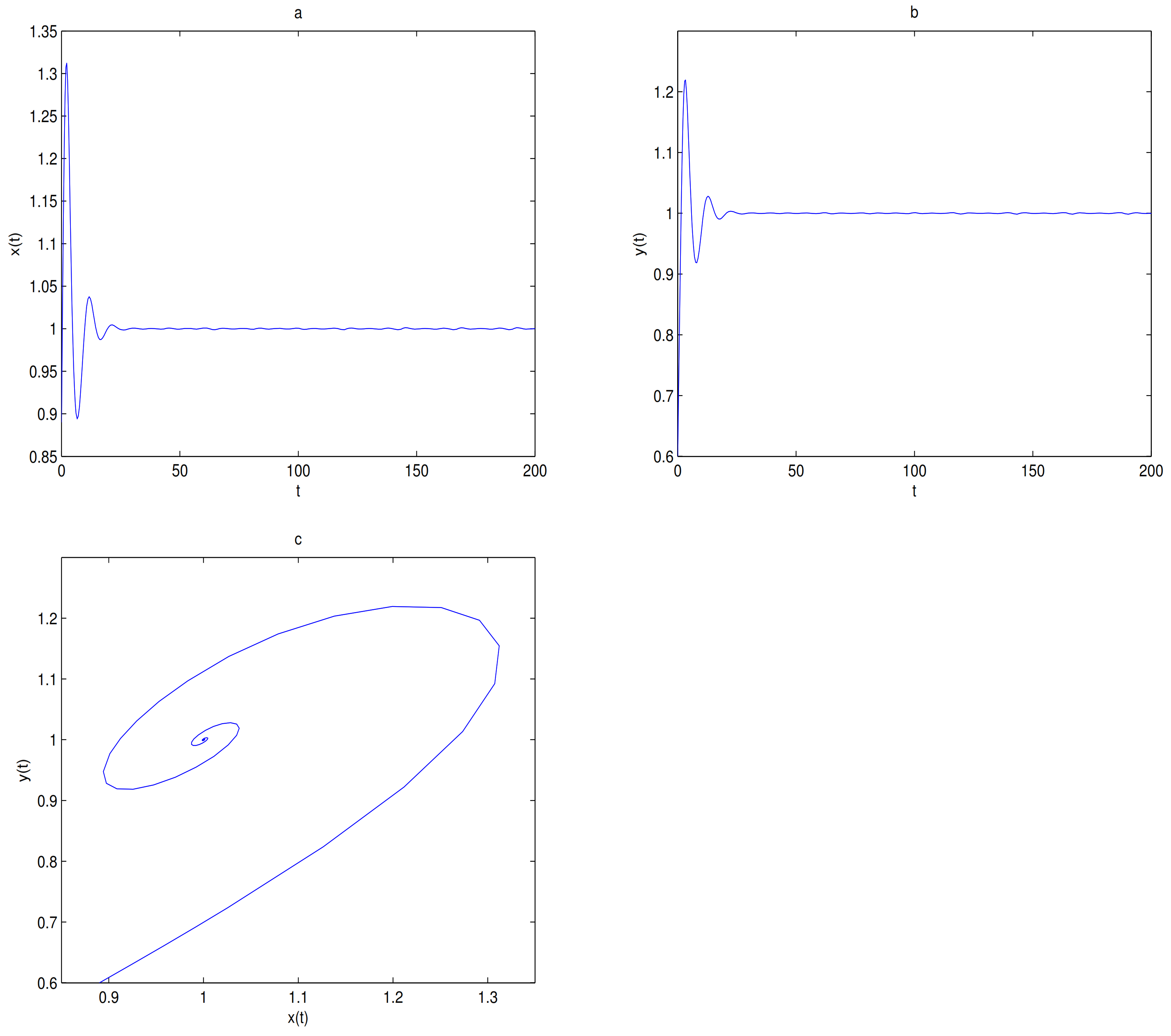
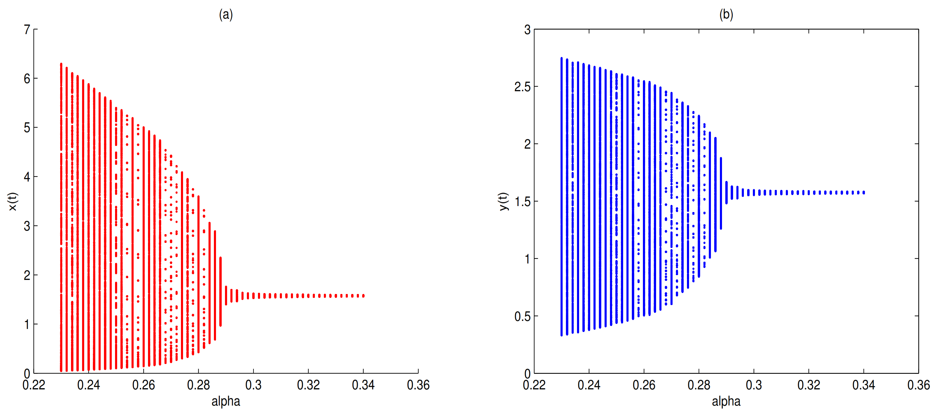
For Theorems 1–3, let $r=1.888,\omega =0.9,b=1$ and $c=1.213$, O is always a saddle. $A_1$ is globally asymptotically stable when $\alpha =0.51$ (see Figure 5) and there exists one limit cycle in $\mathsf{\Omega }$ when $\alpha =0.22$, in here $\left(x\right(0),y(0\left)\right)=(4.7,4.4)$ (see Figure 6). Choosing $\alpha$ as a bifurcation parameter, a supercritical Hopf bifurcation occurs near $A_1$ when $\alpha$ passes through 0.288, in here $\left(x\right(0),y(0\left)\right)=(1.49,1.49)$ (see Figure 7).

Figure 5. The positive equilibrium point $A_1=(1.574,1.574)$ of system (9) is globally asymptotically stable when $r=1.888, \omega =0.9, b=1, c=1.213, \alpha =0.51$. Subfigure (a) is time series of $x\left(t\right)$, subfigure (b) is time series of $y\left(t\right)$, and subfigure (c) is phase diagram of system (9).

Figure 6. There exists a limit cycle in $\mathsf{\Omega }$ when $r=1.888, \omega =0.9, b=1, c=1.213, \alpha =0.22$. $A_1=(1.574,1.574)$. Subfigure (a) is time series of $x\left(t\right)$, subfigure (b) is time series of $y\left(t\right)$, and subfigure (c) is phase diagram of system (9).

Figure 7. There is a supercritical Hopf bifurcation when $\eta$ passes through 0, i.e., $\alpha$ passes through 0.288. Here $r=1.888, \omega =0.9, b=1, c=1.213$, $A_1=(1.574, 1.574)$. Figure (a) is a biurcation diagram of $x\left(t\right)$ with respect to $\alpha$, and Figure (b) is a bifurcation diagram of $y\left(t\right)$ with respect to $\alpha$.

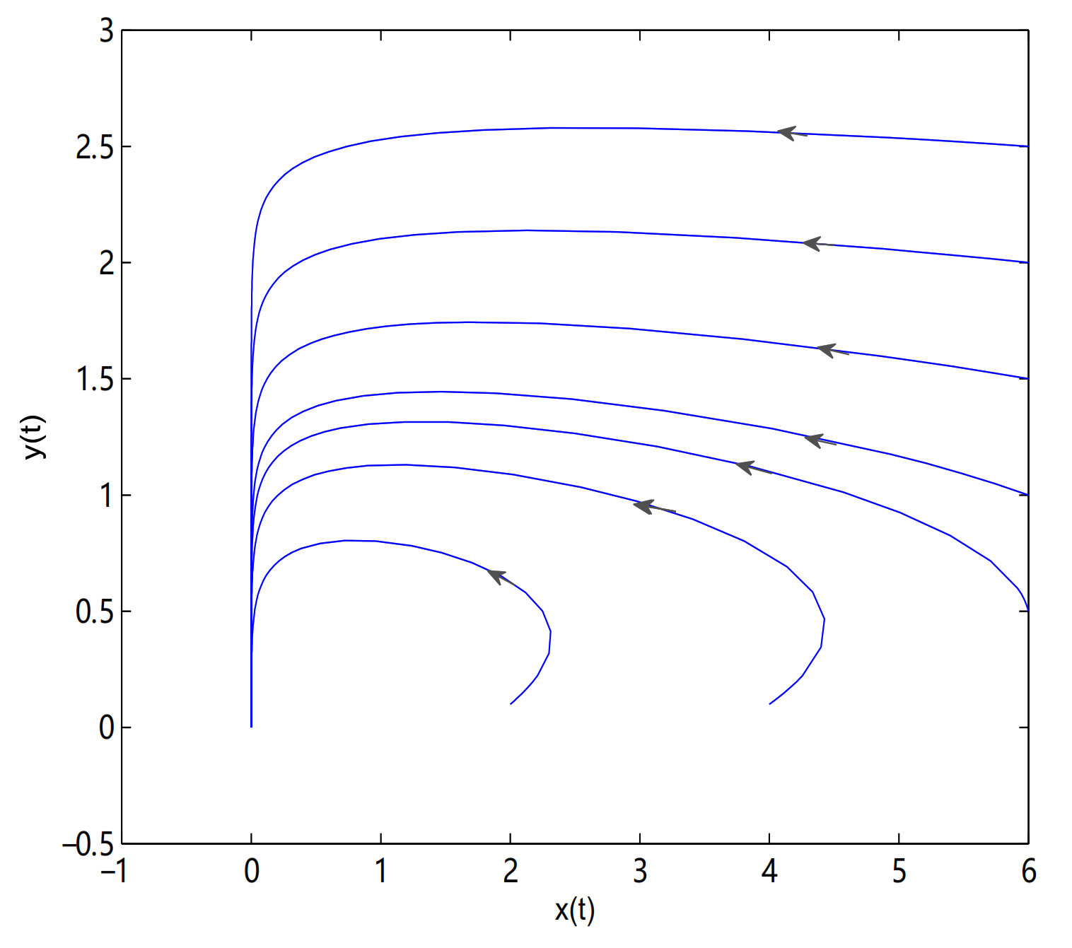
For Theorem 4, let $r=1.5,\omega =3,b=0.5,c=1$ and $\alpha =0.4$, O is the only equilibrium point of system (9) at this time, and O is globally asymptotically stable. In here initial values are (6, 2.5), (6, 2), (6, 1.5), (6, 1), (4, 0.1) and (2, 0.1), we see that all trajectories tend to O (see Figure 8). Let $r=2,\omega =0.414,b=0.5$ and $c=2.87$, O is always locally stable, and $A_2$ is always a saddle. $A_3$ is locally stable when $\alpha =1.674$. the trajectory tends to $A_3$ when the initial value is selected in the attraction domain of $A_3$, for example, $\left(x\right(0),y(0\left)\right)=(4.6,4.6)$ (see Figure 9). The trajectory tends to O when the initial value is selected in the attraction domain of O, for example, $\left(x\right(0),y(0\left)\right)=(1.2,1.4)$ (see Figure 10). 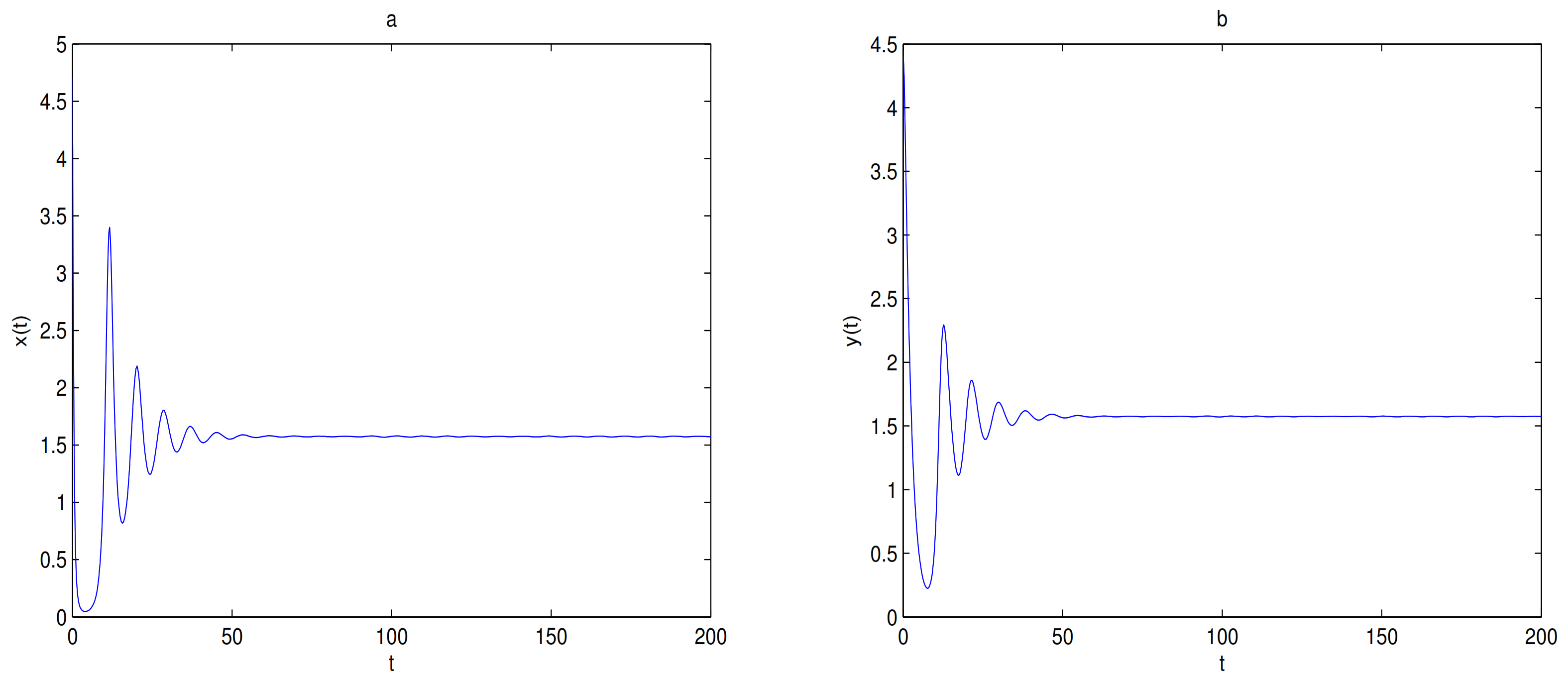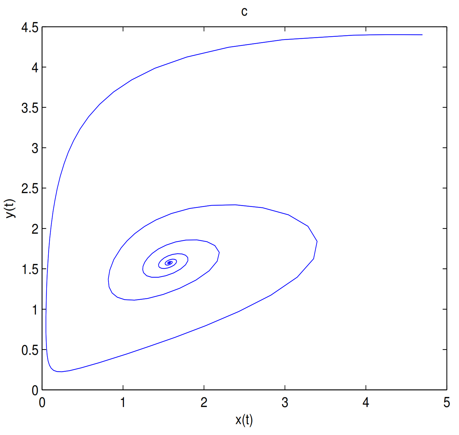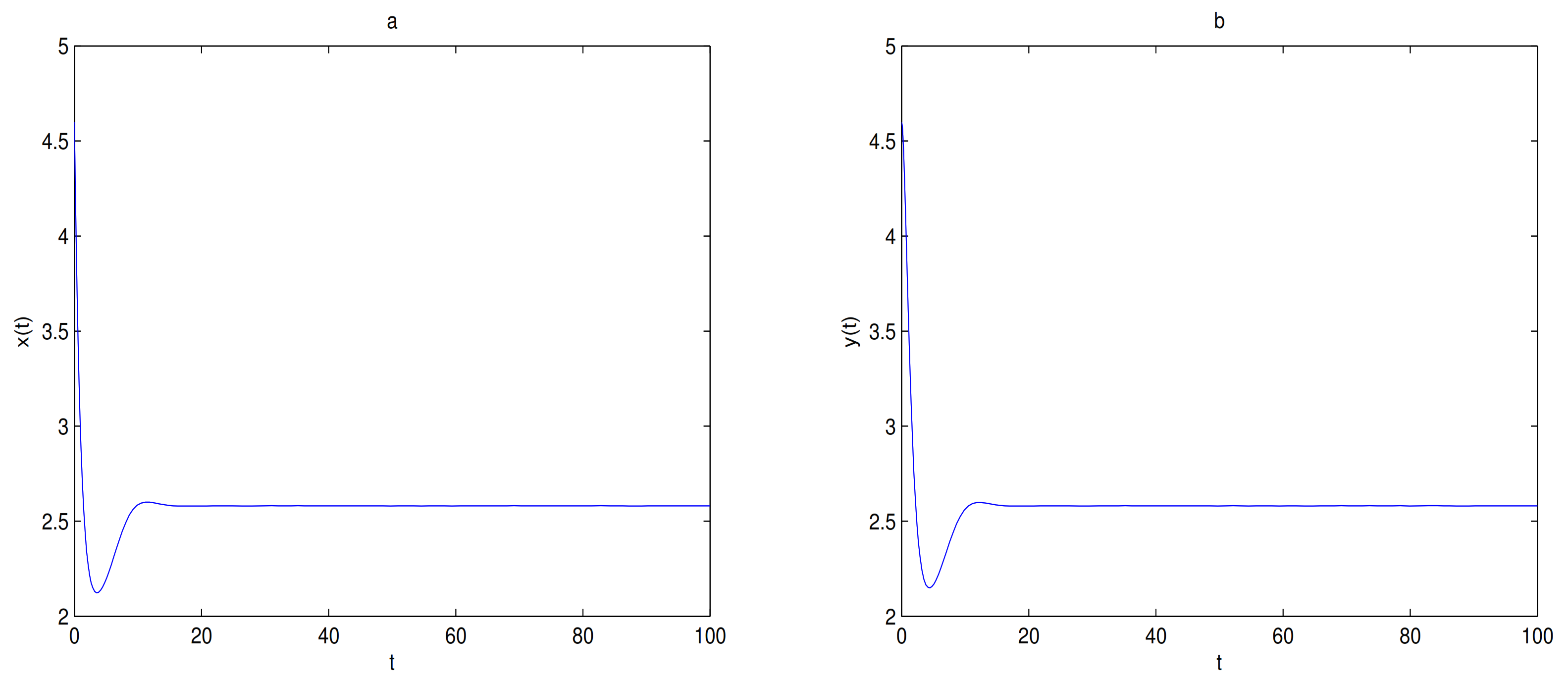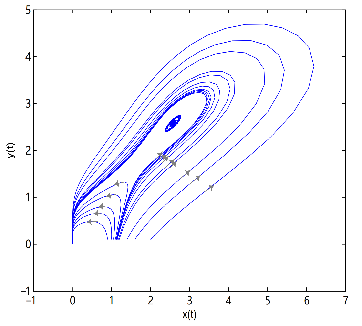$A_3$ is a center-type equilibrium point when $\alpha =0.78$, in here initial values are (2.57, 2.57), (2.42, 2.42), (2.1, 0.1), (1.6, 0.1), (1.4, 0.1), (1.2, 0.1), (1.18, 0.1), (1.15, 0.1), (1.14, 0.1), (1.135, 0.1), (1.133, 0.1), (1.131, 0.1), (1.13, 0.1), (1.1, 0.1), (1.05, 0.1), (1, 0.1) and (0.9, 0.1) (see Figure 11). 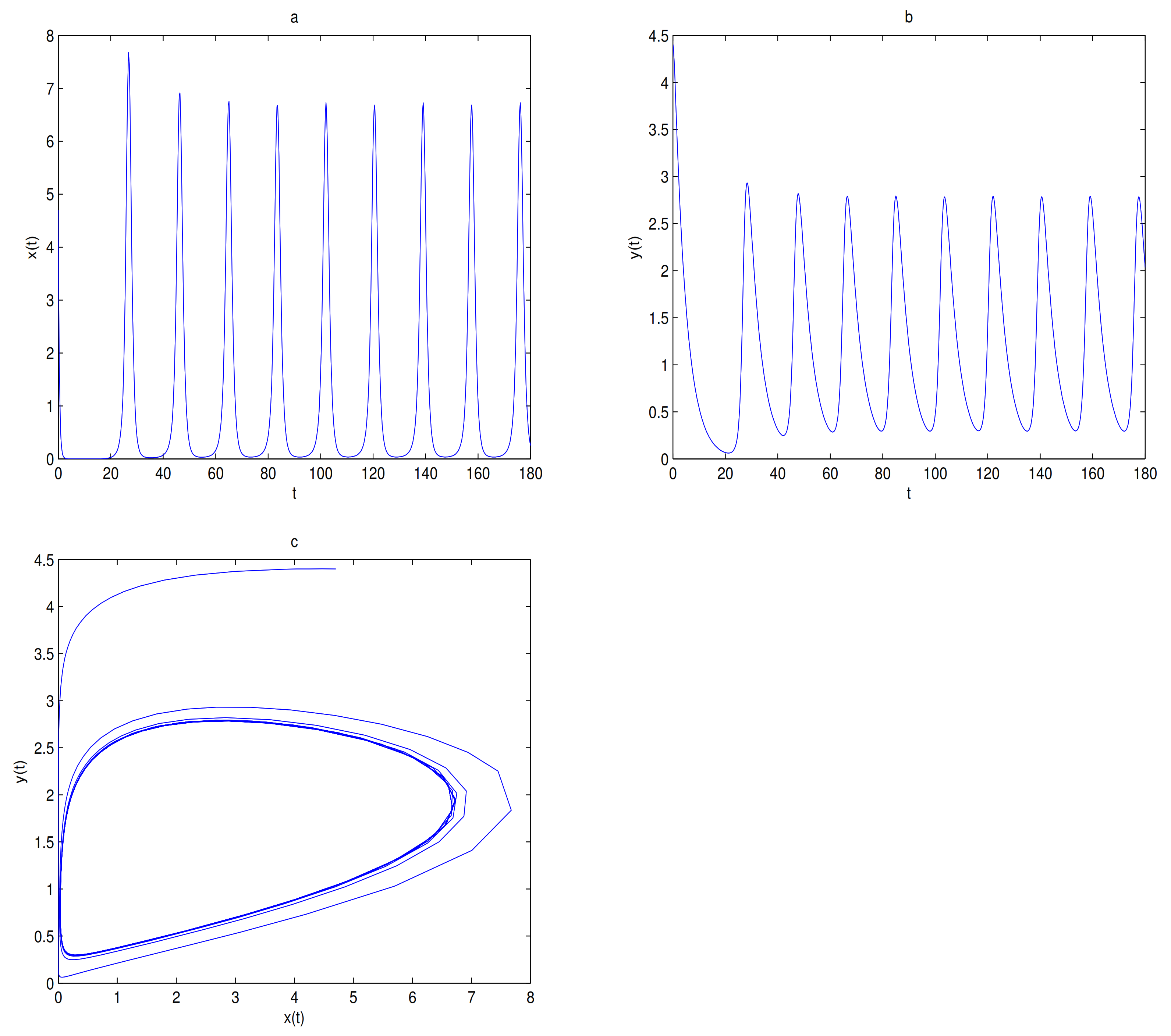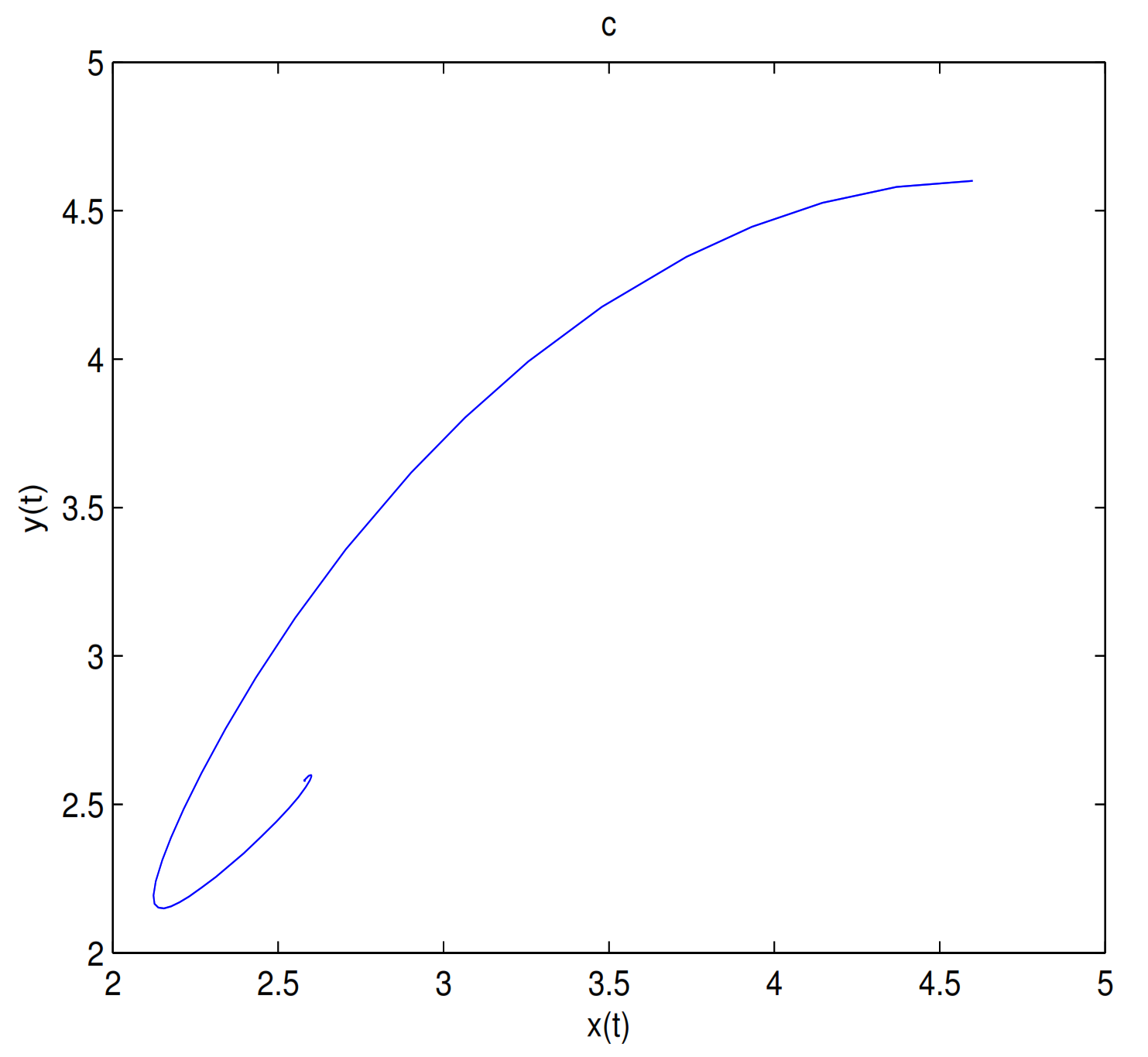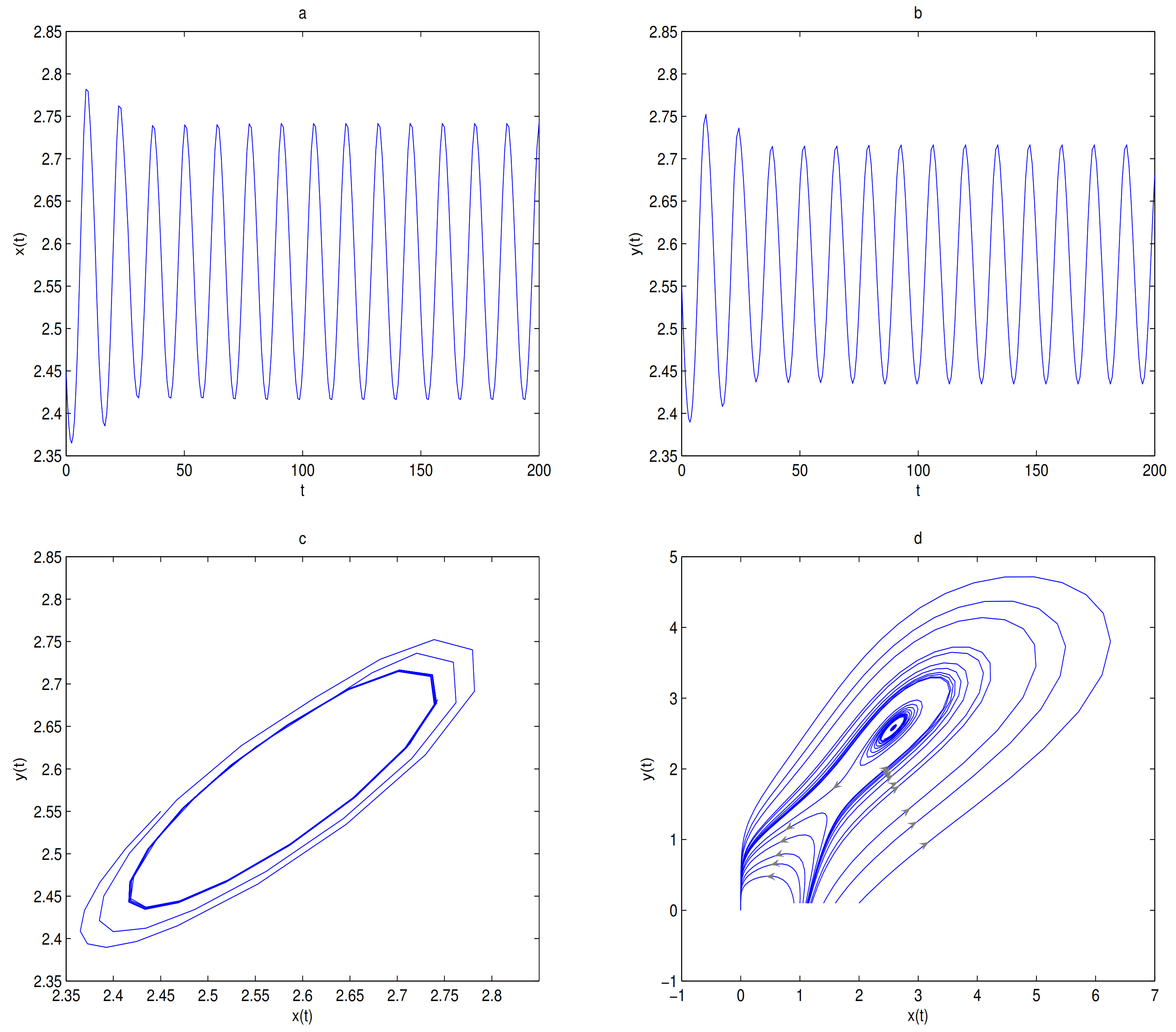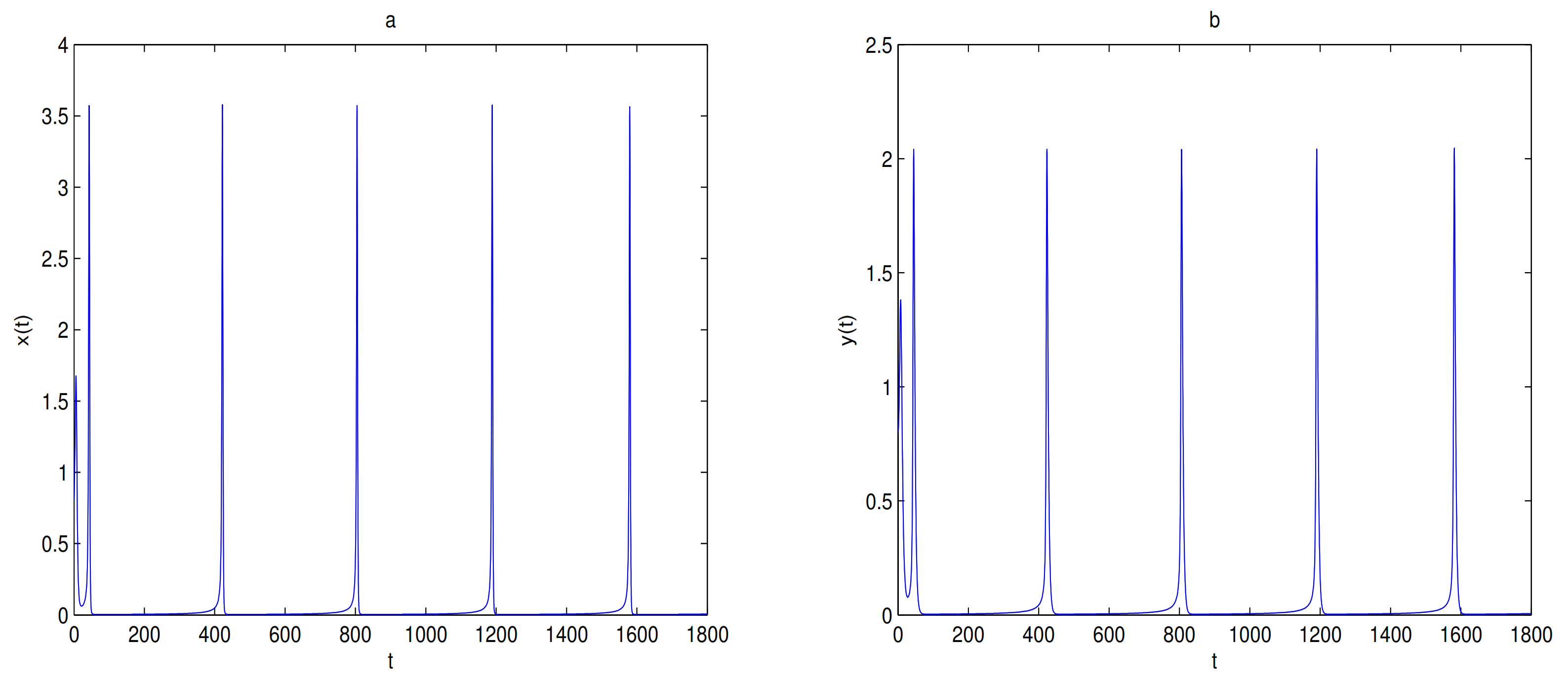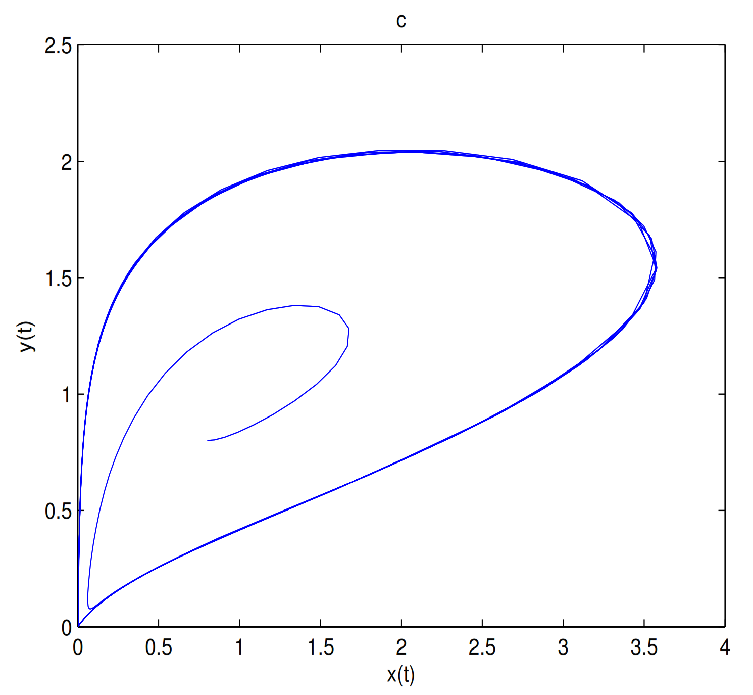$A_3$ is unstable when $\alpha =0.77$, and a limit cycle is generated by Hopf supercritical bifurcation in the neighborhood of $A_3$. We choose $\left(x\right(0),y(0\left)\right)=(2.45,2.55)$ as initial value (see Figure 12c). We choose the same initial values as in Figure 11, and we see that the trajectory forms a limit cycle with (2.57,2.57) as the initial value, and everything else tends to O (Figure 12d).

Figure 8. O is globally asymptotically stable. All trajectories tend to O. In here $r=1.5, \omega =3$, $b=0.5, c=1,\alpha =0.4$.

Figure 9. O is locally stable. $A_2$(1.75, 1.75) is a saddle. $A_3$(2.581, 2.581) is locally stable. The trajectory tends to $A_3$ when the initial value is $\left(x\right(0),y(0\left)\right)=(4.6,4.6)$. In here $r=2, \omega =0.414, b=0.5, c=2.87$, $\alpha =1.674$. Subfigure (a) is time series of $x\left(t\right)$, subfigure (b) is time series of $y\left(t\right)$ and subfigure (c) is phase diagram of system (9).

Figure 10. O is locally stable. $A_2$(1.75, 1.75) is a saddle. $A_3$(2.581, 2.581) is locally stable. The trajectory tends to O when the initial value is $\left(x\right(0),y(0\left)\right)=(1.2,1.4)$. In here $r=2, \omega =0.414, b=0.5$, $c=2.87, \alpha =1.674$. Subfigure (a) is time series of $x\left(t\right)$, subfigure (b) is time series of $y\left(t\right)$, and subfigure (c) is phase diagram of system (9).

Figure 11. O is locally stable. $A_2$(1.75, 1.75) is a saddle. $A_3$(2.581, 2.581) is a center-type equilibrium point. In here $r=2, \omega =0.414, b=0.5, c=2.87, \alpha =0.78$.

Figure 12. Subfigure (a) is time series of $x\left(t\right)$, subfigure (b) is time series of $y\left(t\right)$ and subfigure (c) is phase diagram of system (9). O is locally stable, $A_2$(1.75, 1.75) is a saddle and $A_3$(2.581, 2.581) is unstable. A limit cycle is generated by Hopf supercritical bifurcarion near $A_3$ in subfigure (c), and subfigure (d) shows that directions of these trajectories. In here $r=2, \omega =0.414, b=0.5$, $c=2.87, \alpha =0.77$. The initial value in subfigure (c) is $\left(x\right(0),y(0\left)\right)=(2.45,2.55)$. The initial values in subfigure (d) are the same as in Figure 11.

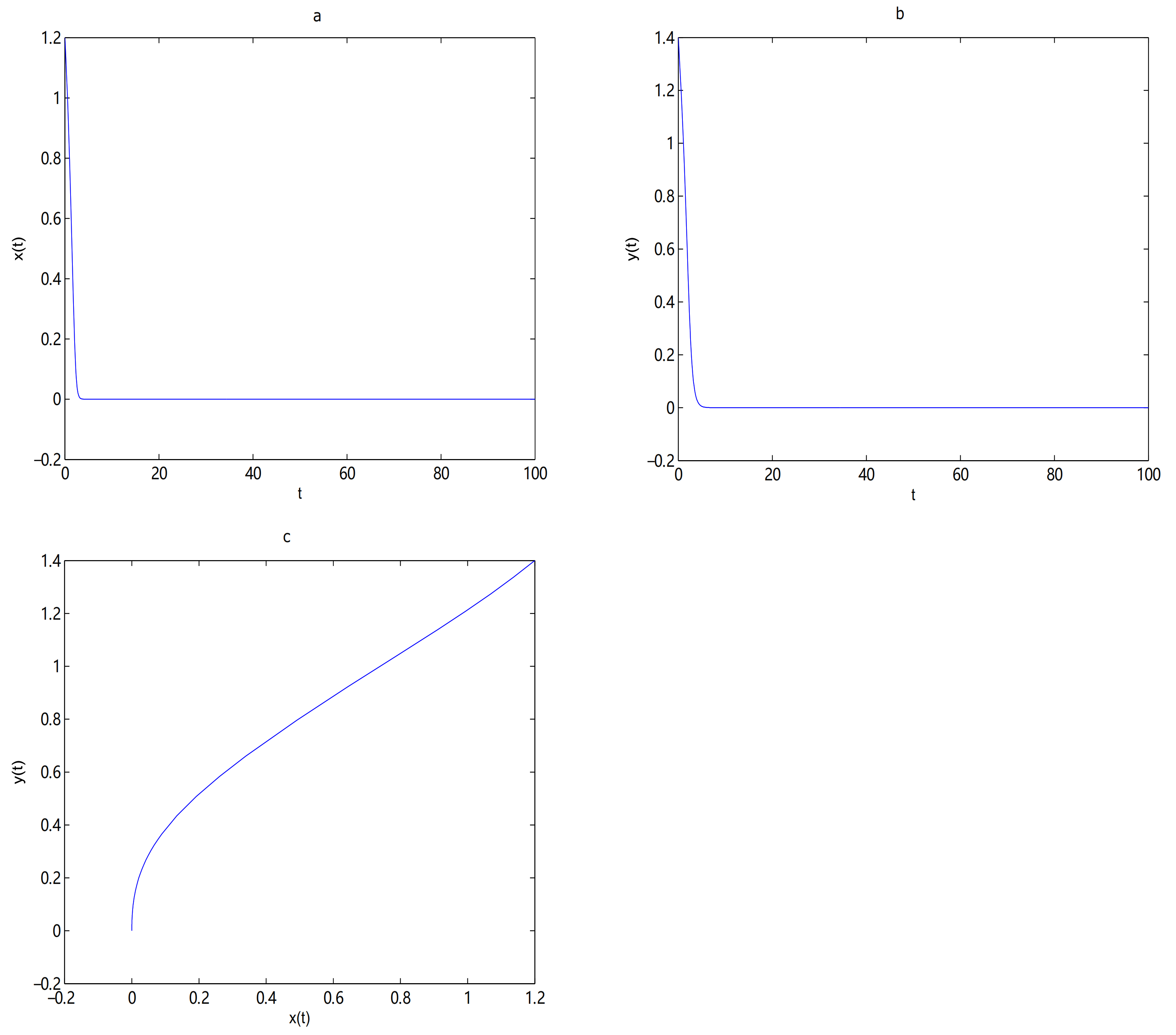
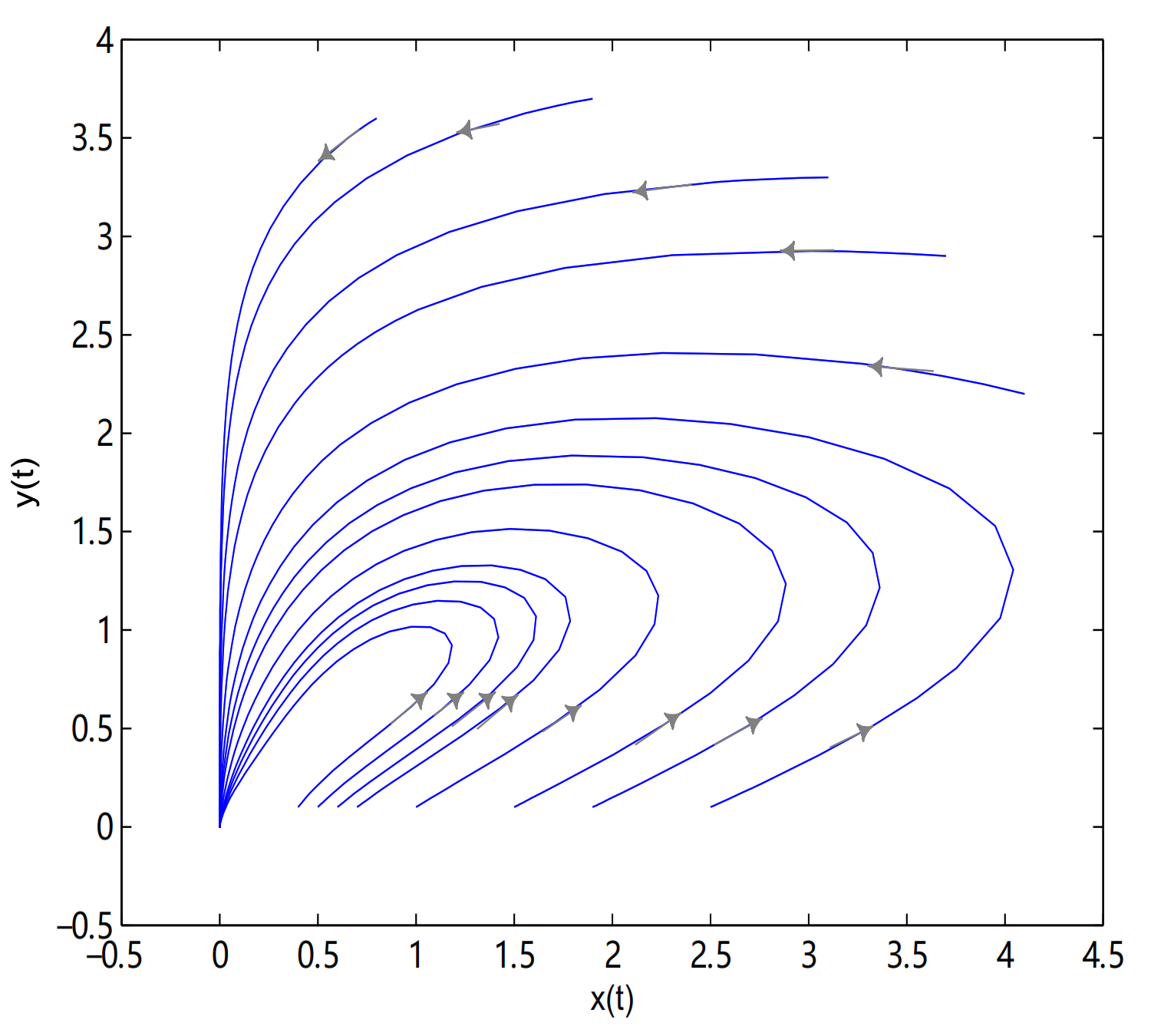
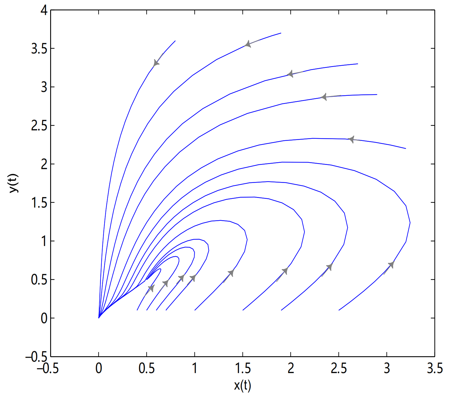
For Theorem 5, let $r=1.5,\omega =1,b=0.5,c=1$, O is always globally asymptotically stable, and $A_2,A_3$ are merged into a single equilibrium $A_4$. Meanwhile, $A_4$ is a saddle node when $\alpha =1$, in here initial values are (2.7, 3.3), (2.9, 2.9), (0.8, 3.6), (3.2, 2.2), (1.9, 3.7), (2.5, 0.1), (1.9, 0.1), (1.5, 0.1), (1, 0.1), (0.7, 0.1), (0.6, 0.1), (0.5, 0.1) and (0.4, 0.1) (see Figure 13). $A_4$ is a degenerate critical point when $\alpha =0.5$, in here initial values are (3.1, 3.3), (3.7, 2.9), (0.8, 3.6), (4.1, 2.2), (1.9, 3.7), (2.5, 0.1), (1.9, 0.1), (1.5, 0.1), (1, 0.1), (0.7, 0.1), (0.6, 0.1), (0.5, 0.1) and (0.4, 0.1) (see Figure 14).

Figure 13. O is globally asymptotically stable. $A_4$(0.5, 0.5) is a saddle node. In here $r=1.5, \omega =1$, $b=0.5, c=1, \alpha =1$.

Figure 14. O is globally asymptotically stable. $A_4$(0.5, 0.5) is a degenerate critical point. In here $r=1.5, \omega =1, b=0.5, c=1, \alpha =0.5$.

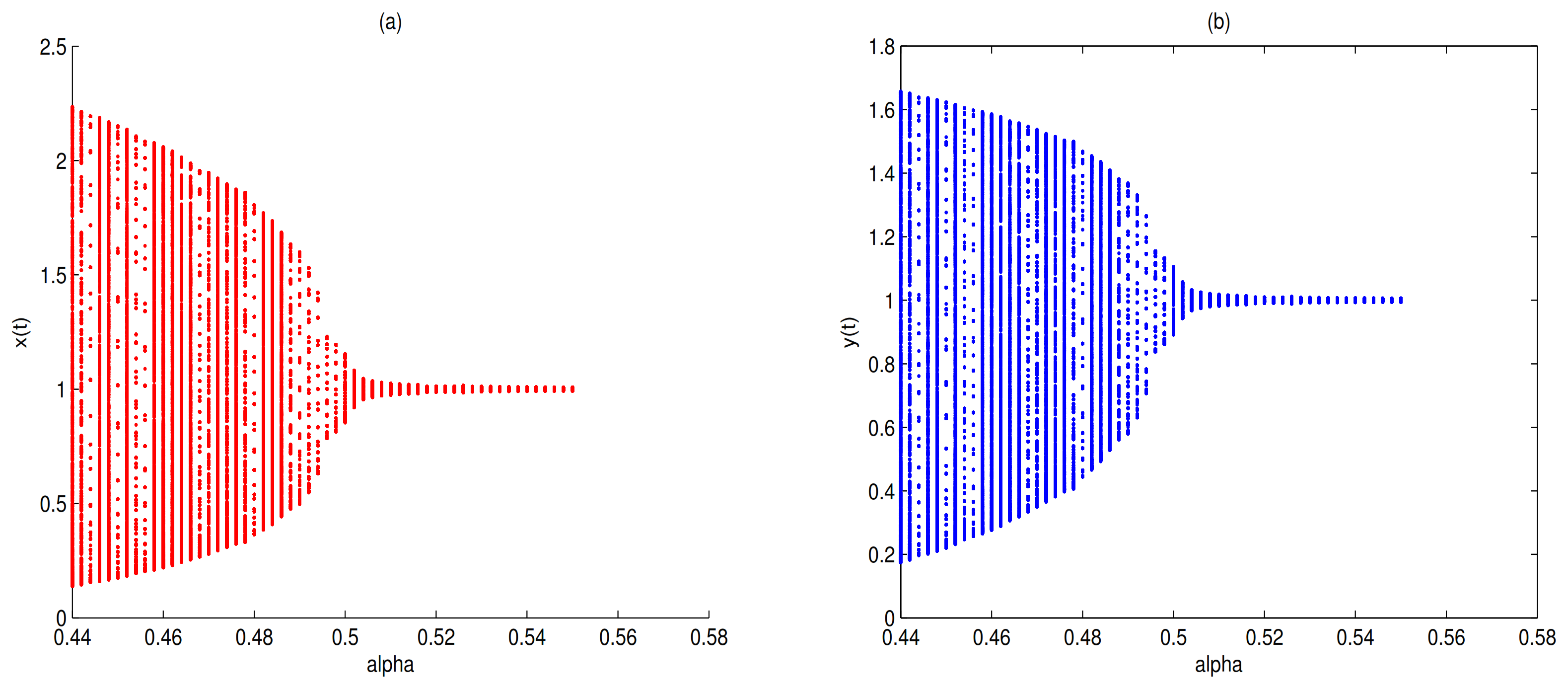
For Theorems 6–8, first, let $r=2,\omega =1,b=1$ and $c=2$; O is always a saddle node. $A_5$ is unstable and there exists a limit cycle near $A_5$ when $\alpha =0.3$, the initial value is (0.8, 0.8) (see Figure 15). $A_5$ is locally stable when $\alpha =0.93$, and the initial value is (0.89, 0.6) (see Figure 16). 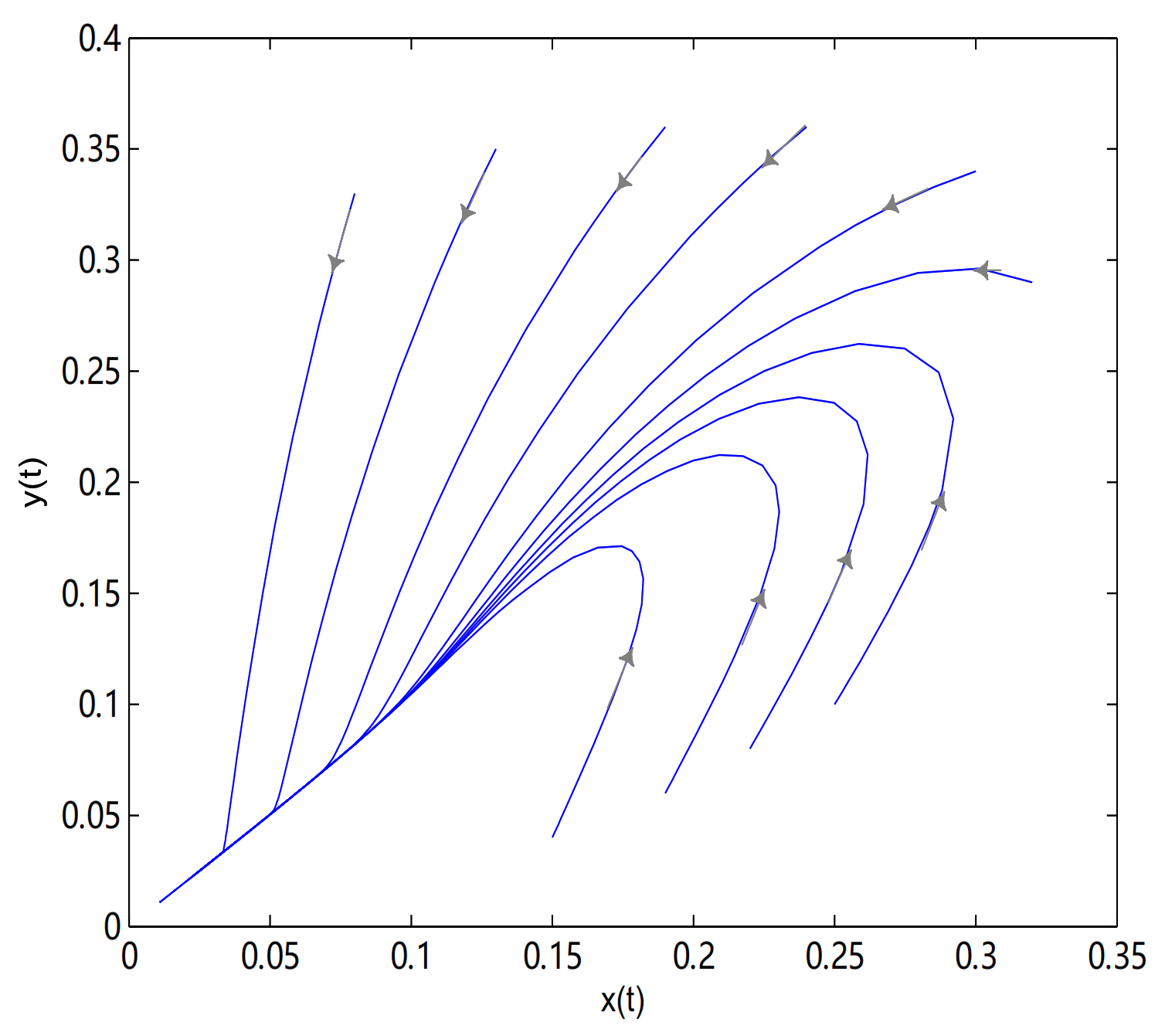By choosing $\alpha$ as a bifurcation parameter, a supercritical Hopf bifurcation occurs near $A_5$ when $\alpha$ passes through 0.5 (see Figure 17). Let $r=2,\omega =2,b=1,c=2$ and $\alpha =0.7$, O is an unstable node, in here initial values are (0.28, 0.34), (0.32, 0.29), (0.19, 0.06), (0.25, 0.1), (0.13, 0.35), (0.08, 0.33), (0.24, 0.36), (0.22, 0.08), (0.15, 0.04) and (0.19, 0.36), all trajectories tend to singular line $y=x$ (see Figure 18).

Figure 15. O is a saddle node, and there exists at least one limit cycle near $A_5(1,1)$. In here $r=2, \omega =1, b=1, c=2, \alpha =0.3$. Subfigure (a) is time series of $x\left(t\right)$, subfigure (b) is time series of $y\left(t\right)$ and subfigure (c) is phase diagram of system (9).

Figure 16. O is a saddle node. $A_5(1,1)$ is locally stable. In here $r=2, \omega =1, b=1, c=2, \alpha =0.93$. Subfigure (a) is time series of $x\left(t\right)$, subfigure (b) is time series of $y\left(t\right)$, and subfigure (c) is a phase diagram of system (9).

Figure 17. There is a supercritical Hopf bifurcation when $\xi$ passes through 0, i.e., $\alpha$ passes through 0.5. In here $r=2, \omega =1, b=1, c=2$. $\left(x\right(0),y(0\left)\right)=(0.9,0.9)$. $A_5(1,1)$. Subigure (a) is a bifurcation diagram of $x\left(t\right)$ with respect to $\alpha$ and subfigure (b) is a bifurcation diagram of $y\left(t\right)$ with respect to $\alpha$.

Figure 18. O is an unstable node. The trajectories tend to $y=x$. In here $r=2, \omega =2, b=1$, $c=2, \alpha =0.7$.

7. Conclusions

In this paper, we established a single population with distributed delay and nonlinear harvesting. Sufficient conditions of existence and stability of equilibria in three different cases have been derived. We presented the results in Table 1. We choose $\omega {\int }_{-\infty }^t\alpha exp(-\alpha (t-s))x\left(s\right)\mathrm{d}s$ as a function for the impact of distributed delay, and choose $\frac{cx\left(t\right)}{b+x\left(t\right)}$ as a function for the harvest. Since this type of harvest exists in the ecosphere especially for vertebrates, and single species population model with distributed delay and Michaelis-Menten type harvesting has never been considered and studied by other scholars, our work is novel. Our results show that the qualitative conclusions obtained are rich and have certain guiding significance for some species with nonlinear harvest. In the future work, we will study single-species models with other harvesting types, such as $\frac{B{x}^2}{A^2+x^2}$, etc.

Table 1. The results under different conditions.

Conditions	Subconditions	Equilibria	Stability
br − c > 0	η < 0	O, $A_1$	O is a saddle, A1 is globally asymptotically stable.
	η > 0	$O,A_1$	O is a saddle, $A_1$ is unstable, there exists at least one limit cycle in Ω.
	η > 0 condition (H1)	$O,A_1$	O is a saddle, $A_1$ is unstable, there exists a unique limit cycle in Ω.
	η = 0 condition (H1)	O, A1	O is a saddle, A1 is center-type, a supercritical Hopf bifurcation occurs near A1.
br − c < 0	$r-\omega b = 0$	O	O is globally asymptotically stable.
	$q^2 > 0,r - \omega b > 0,\beta < 0$	O, A2, A3	O is locally stable, A2 is a saddle, A3 is locally stable.
	$q^2 > 0,r - \omega b > 0,\beta > 0$	O, $A_2$, $A_3$	O is locally stable, A2 is a saddle, A3 is unstable.
	$q^2 > 0,r - \omega b > 0,\beta = 0$ and condition (H2)	$O,A_2$, $A_3$	O is locally stable, $A_2$ is a saddle, a supercritical Hopf bifurcation occurs near A3.
	$$\begin{gathered} q^2 = 0,r - \omega b > 0, \\ r - \omega b- 2\alpha \ne 0 \end{gathered}$$	$O,A_4$	O is globally asymptotically stable, A4 is a saddle node.
	$$\begin{gathered} q^2 = 0,r - \omega b > 0, \\ r - \omega b- 2\alpha = 0 \end{gathered}$$	O, A4	O is globally asymptotically stable, A4 is a degenerate critical point.
br − c = 0	$r-\omega b>0,\xi >0$	O, $A_5$	O is a saddle node, A5 is unstable, there exists at least one limit cycle near A5.
	$r-\omega b>0,\xi <0$	$O,A_5$	O is a saddle node, $A_5$ is locally stable.
	$r-\omega b>0,\xi =0$ and condition (H3)	$O,A_5$	O is a saddle node, $A_5$ is unstable, a supercritical Hopf bifurcation occurs near A5.
	$r-\omega b = 0$	O	O is an unstable node, system (9) has a singular line y = x.