Issues on Applying One- and Multi-Step Numerical Methods to Chaotic Oscillators for FPGA Implementation

Abstract

Chaotic oscillators have been designed with embedded systems like field-programmable gate arrays (FPGAs), and applied in different engineering areas. However, the majority of works do not detail the issues when choosing a numerical method and the associated electronic implementation. In this manner, we show the FPGA implementation of chaotic and hyper-chaotic oscillators from the selection of a one-step or multi-step numerical method. We highlight that one challenge is the selection of the time-step h to increase the frequency of operation. The case studies include the application of three one-step and three multi-step numerical methods to simulate three chaotic and two hyper-chaotic oscillators. The numerical methods provide similar chaotic time-series, which are used within a time-series analyzer (TISEAN) to evaluate the Lyapunov exponents and Kaplan–Yorke dimension ($D_{KY}$) of the (hyper-)chaotic oscillators. The oscillators providing higher exponents and $D_{KY}$ are chosen because higher values mean that the chaotic time series may be more random to find applications in chaotic secure communications. In addition, we choose representative numerical methods to perform their FPGA implementation, which hardware resources are described and counted. It is highlighted that the Forward Euler method requires the lowest hardware resources, but it has lower stability and exactness compared to other one-step and multi-step methods.

1. Introduction

Chaos is a nonlinear and unpredictable behavior that can be modeled by ordinary differential equations (ODEs). In continuous-time, the minimum number of ODEs for autonomous chaotic oscillators is three, as for example in [1,2]. A dynamical system modeled by four or more ODEs can generate hyper-chaotic behavior, as for example in [3]. Although sensitivity to initial conditions does not necessarily yield chaos [4], the majority of authors agree that the main characteristic of a dynamical system that generates chaos is the high sensibility to initial conditions, which is associated with a high unpredictability in the evolution of the time series of the state variables. The chaotic time series can be used to estimate Lyapunov exponents, as already shown in the seminal work [5], and by using the software for TIme SEries ANalysis (TISEAN) introduced in [6]. Lyapunov exponents are quite useful to characterize the behavior of a dynamical system, and they quantify the exponentially fast divergence or convergence of nearby orbits that can be seen in phase space.

Nowadays, it is said that a system with one positive Lyapunov exponent (LE+) is defined to be chaotic, and a system with more than one LE+ is hyper-chaotic. Some engineering applications of chaotic oscillators can be found in [7], which provides guidelines on the implementation by using field-programmable gate arrays (FPGAs), and shows the design of random number generators (RNGs) and chaotic secure communication systems [8]. The applications based on (hyper-)chaotic oscillators can be enhanced by guaranteeing higher unpredictability of the chaotic time series. One way is finding the chaotic oscillator having the highest LE+ [2], and also one must take into account other dynamical characteristics such as entropy and Kaplan–Yorke dimension ($D_{KY}$). For a chaotic oscillator having three ODEs, one computes three Lyapunov exponents, where one must be positive, one zero and one negative. There are methods to evaluate the Lyapunov spectrum [9,10], the seminal one was introduced in [5], and herein we apply TISEAN [6].

Recent works show the usefulness of chaotic oscillators in different engineering problems [11,12,13], however, there is no information on the issues related to the implementation of the numerical methods in electronic systems. In this manner, this paper uses three representative chaotic and two hyper-chaotic oscillators as case studies, which are listed in Table 1, along with their associated name, ODEs and parameter values that are used herein to generate chaotic behavior. The five chaotic oscillators are case studies to evaluate LE+ and $D_{KY}$ from their chaotic time series that are generated by applying three one-step and three multi-step methods. Representative numerical methods are chosen to be implemented on a FPGA and their hardware resources are counted to show the challenges of minimizing hardware resources while guaranteeing the highest exactness and stability of the numerical simulations.

Table 1. Chaotic and hyper-chaotic oscillators.

Name	ODEs	Parameters
CO1 [1]	$\begin{array}{c}\dot{x}=\sigma (y-x)\hfill \\ \dot{y}=x(\rho -z)-y\hfill \\ \dot{z}=xy-\beta z\hfill \end{array}$	$\begin{array}{c}\sigma =10,\beta =8/3,\hfill \\ \rho =28\hfill \end{array}$
CO2 [1]	$\begin{array}{c}\dot{x}=-y-z\hfill \\ \dot{y}=x+ay\hfill \\ \dot{z}=b+z(x-c)\hfill \end{array}$	$\begin{array}{c}a=b=0.2,\hfill \\ c=5.7\hfill \end{array}$
CO3 [2]	$\begin{array}{c}\dot{x}=y\hfill \\ \dot{y}=z\hfill \\ \dot{z}=-ax-by-cz\hfill \\ +d_{1}f(x,m)\hfill \end{array}$	$\begin{array}{c}a=0.7,b=0.7,\hfill \\ c=0.7,d_1=0.7\hfill \end{array}$
HO4 [3]	$\begin{array}{c}\dot{x}=a(y-x)+yz+w\hfill \\ \dot{y}=by+cxz-p{x}^2+w\hfill \\ \dot{z}=xy-d\hfill \\ \dot{w}=-x-y\hfill \end{array}$	$\begin{array}{c}a=16,b=3,\hfill \\ c=8,d=20,\hfill \\ p=0.1\hfill \end{array}$
HO5 [17]	$\begin{array}{c}\dot{x}=a(y-x)-w\hfill \\ \dot{y}=bx+2y+xz\hfill \\ \dot{z}=c-xy\hfill \\ \dot{w}=x\hfill \end{array}$	$\begin{array}{c}a=6,b=5,\hfill \\ c=50\hfill \end{array}$

The three chaotic and two hyper-chaotic oscillators that are case studies in this paper are detailed in Section 2. Three one-step and three multi-step numerical methods are given in Section 3. The chaotic time series of each state variable of each (hyper-)chaotic oscillator are generated by applying all the numerical methods, and the LE+ and $D_{KY}$ of each state variable are evaluated in Section 4. The FPGA implementation of representative numerical methods is detailed in Section 5. Finally, the conclusions are summarized in Section 6.

2. Chaotic and Hyper-Chaotic Oscillators

The three chaotic (modeled by three ODEs) and two hyper-chaotic (modeled by four ODEs) oscillators that are case studies herein are given in Table 1. In this Table CO1 is the well-known Lorenz system, introduced in 1963 as a simplified mathematical model for atmospheric convection [14], and from which was accidentally discovered the property associated to the high sensitivity to initial conditions. This originated one of the main characteristics in chaos theory and this CO1 is widely used as a work-horse to verify simulation and hardware implementation issues. In phase space, the Lorenz attractor resembles a butterfly effect, which stems from the real-world implications, i.e., in any physical system, the prediction of the evolution of the chaotic trajectories of the state variables will always fail in the absence of perfect knowledge of the initial conditions. In this manner, although physical systems can be completely deterministic, their chaotic behavior makes them inherently unpredictable (https://en.wikipedia.org/wiki/Lorenz_system#cite_note-lorenz-1).

The chaotic oscillator labeled as CO2 is another well-known system introduced by Otto Rössler in 1976, originally intended to behave similarly to the Lorenz attractor, but its dynamical behavior is simpler and has only one manifold. In the Rössler system, an orbit within the attractor follows an outward spiral around an unstable fixed point. From the mathematical model of CO2 given in Table 1, this spiral effect is seen in the $x,y$ plane, and once the graph spirals out enough, the z-dimension shows the influence of a second fixed point causing rise and twist. After the introduction of the Rössler system, important news was that the original model was useful in modeling equilibrium in chemical reactions [15].

CO3 is based on a saturated nonlinear function series that can be approximated by a piecewise-linear (PWL) function. Considering that the PWL function has saturation levels $k_i$, break-points $B_i$ and slope m, then Equation (1) can be used to generate two scrolls, and Equation (2) to generate three scrolls. In a general sense, the PWL function given in Equation (1) can be increased to generate an even number of scrolls, and Equation (2) to generate an odd number of scrolls, as shown in [16].

The hyper-chaotic oscillators labeled as HO4 and HO5, both have more than three ODEs in order to have more than one positive Lyapunov exponent, so that they present a more complex behavior than chaotic oscillators modeled by three ODEs.

$$f\left(x\right)=\left\{\begin{array}{cc}{k}_1& \mathrm{if}{B}_1<x<B_2\\ mx& \mathrm{if}{B}_2\le x\le B_3\\ k_2& \mathrm{if}{B}_3<x<B_4\end{array}\right.$$

(1)

$$f\left(x\right)=\left\{\begin{array}{cc}{k}_1& \mathrm{if}{B}_1<x<B_2\\ m\left(x-\frac{B_2+B_3}{2}-\frac{k_1+k_2}{2}\right)& \mathrm{if}{B}_2\le x\le B_3\\ k_2& \mathrm{if}{B}_3<x<B_4\\ m\left(x-\frac{B_4+B_5}{2}-\frac{k_2+k_3}{2}\right)& \mathrm{if}{B}_4\le x\le B_5\\ k_3& \mathrm{if}{B}_5<x<B_6\end{array}\right.$$

(2)

3. One-Step and Multi-Step Methods

The mathematical models of the chaotic and hyper-chaotic oscillators given in Table 1 can be formulated as initial value problems of the type $\dot{x}=f\left(x\right)$. The solution of the ODEs can be performed by applying one-step and multi-step methods. The former requires values evaluated in one step $x_i$ to evaluate the next step denoted by $x_{i+1}$, while the multi-step methods require two or more previous step values denoted as $x_i,x_{i-1},x_{i-2,\cdots }$ to evaluate $x_{i+1}$. Other classifications are predictor or explicit and corrector or implicit methods. The explicit methods require past steps to evaluate the current step at iteration $i+1$, but the implicit methods require estimation of the value at the current step $i+1$ and past values at steps $x_i,x_{i-1},x_{i-2,\cdots }$. In this manner, it is common to name predictor–corrector [18] to the implicit methods, and they require an explicit method to evaluate the functions at the current iteration.

The explicit methods are faster than the implicit ones, but they may present numerical instability and lower exactness than the implicit methods. There are some rules for choosing the explicit method that is used within an implicit one to evaluate the current step $x_{i+1}$ [18]. The step-size can also be varied during the computation or it can be constant and can be estimated from the stability analysis of the method, but one must take care of choosing the correct step-size to avoid non-convergence [19]. The explicit or predictor is the weak part in an implicit method due to the inherent truncation error, so that it puts a condition on the exactness of the initial prediction and the step-size of the corrector [18]. To enhance FPGA implementations of the numerical methods, the challenge is the selection of a method that allows a large step-size. That way, the larger the step-size of a numerical method, the higher the operating frequency of the FPGA implementation, as shown in Section 5.

The solution of the five chaotic oscillators given in the previous section are solved herein by applying the three one-step methods given in Table 2, and the three multi-step methods given in Table 3. The one-step methods are labeled as Forward Euler (FE), Backward Euler (BE) and fourth-order Runge–Kutta (RK4). The multi-step methods are labeled as sixth-order Adams–Bashforth (AB6), fourth-order Adams–Moulton (AM4) and fourth-order Gear (G4).

Table 2. One-step methods.

Method	Iterative Equation
Forward Euler (FE)	$y_{i+1}=y_i+hf(y_i,t_i)$
Backward Euler (BE)	$y_{i+1}=y_i+hf(y_{i+1},t_{i+1})$
Runge–Kutta 4 (RK4)	$\begin{array}{c}{k}_1=hf(x_i,y_i)\hfill \\ k_2=hf(x_i+\frac{1}{2}h,y_i+\frac{1}{2}{k}_1),\hfill \\ k_3=hf(x_i+\frac{1}{2}h,y_i+\frac{1}{2}{k}_2),\hfill \\ k_4=hf(x_i+h,y_i+k_3),\hfill \\ y_{i+1}=y_i+\frac{1}{6}(k_1+2k_2+2k_3+k_4)\hfill \end{array}$

Table 3. Multi-step methods.

Method	Iterative Equation
Adams– Bashforth 6 (AB6)	$\begin{array}{c}{y}_{i+1}=y_i+\frac{h}{1440}(4277f(t_i,y_i)\hfill \\ -7923f(t_{i-1},y_{i-1})+9982f(t_{i-2},y_{i-2})\hfill \\ -7298f(t_{i-3},y_{i-3})+2877f(t_{i-4},y_{i-4})\hfill \\ -475f(t_{i-5},y_{i-5}))\hfill \end{array}$
Adams– Moulton 4 (AM4)	$\begin{array}{c}{y}_{i+1}=y_i+\frac{h}{24}(9f(t_{i+1},y_{i+1})\hfill \\ +19f(t_i,y_i)-5f(t_{i-1},y_{i-1})\hfill \\ +f(t_{i-2},y_{i-2}))\hfill \end{array}$
Gear 4 (G4)	$\begin{array}{c}{y}_{i+1}=\frac{48}{25}{y}_i+-\frac{36}{25}{y}_{i-1}\hfill \\ +\frac{16}{25}{y}_{i-2}-\frac{3}{25}{y}_{i-3}\hfill \\ +\frac{12}{25}hf\left(y_{i+1}\right)\hfill \end{array}$

4. Chaotic Time Series, LE+ and ${\mathbf{D}}_{\mathbf{KY}}$

In Table 1, CO1 is the well-known Lorenz system, therefore, we show the simulation results for CO2, CO3, HO4 and HO5. The step-size h for each numerical method is given in the upper corner of each figure. One can appreciate that in some cases h is decreased to generate the same behavior provided by the majority of methods. Although the time evolution of the chaotic series is different for each method, the LE+ and $D_{KY}$ are similar, and it can be improved by varying h, which is not a trivial task and requires the analysis of the eigenvalues associated to each Jacobian matrix of each equilibrium point of each chaotic oscillator.

Figure 1, Figure 2, Figure 3 and Figure 4 show some chaotic time series of the (hyper-)chaotic oscillators simulated by applying the six numerical methods and listing the step-size h. The six methods were programmed into MatLab, and afterwards described in hardware language for FPGA implementation. In this case, a large h is desired to increase the operation frequency of an FPGA implementation, as shown in the following section.

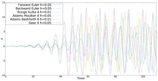
Figure 1. Time series of x of CO2 given in Table 1 with initial conditions $x_0=y_0=z_0=0.01$.

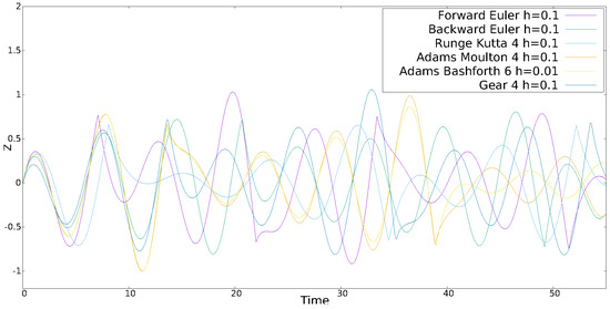
Figure 2. Time series of z of CO3 given in Table 1 with initial conditions $x_0=y_0=0.1,z_0=0.0$.

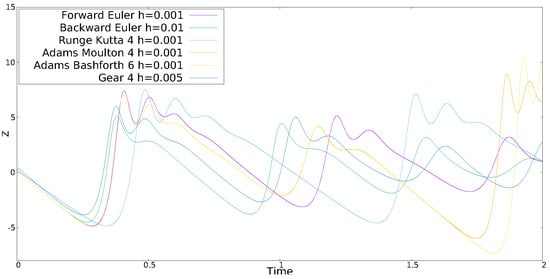
Figure 3. Time series of z of HO4 given in Table 1 with initial conditions $x_0=y_0=z_0=w_0=0.2$.

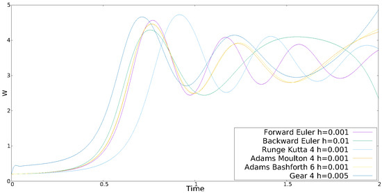
Figure 4. Time series of w of HO5 given in Table 1 with initial conditions $x_0=y_0=z_0=w_0=0.2$.

The $D_{KY}$ is evaluated from the Lyapunov exponents [9], and for an n-dimensional system it is evaluated by Equation (3), where $L{E}_1,\dots ,L{E}_n$ are Lyapunov exponent values ordered from the highest to the lowest value.

$$D_{KY}=(n-1)+{\displaystyle \frac{L{E}_1+L{E}_2+L{E}_{n-1}}{|L{E}_n|}}$$

(3)

The LE+ and $D_{KY}$ were evaluated by TISEAN [6], which is based on the method introduced in [20]. The parameters for TISEAN are different for each state variable and analysis is performed using 50,000 samples for each chaotic time series. The LE+ for each state variable of each oscillator is shown in Table 4, and ordered from the highest to the lowest value. The highest LE+ is from the state variable x of HO4 and simulated with the fourth-order Runge–Kutta method, so that it is labeled as x_HO4_RK4. The same labels were adopted for the evaluation of $D_{KY}$, whose results are shown in Table 5.

Table 4. LE+ (ordered from the highest to the lowest) evaluated by time series analysis (TISEAN) for each state variable of the five oscillators given in Table 1, and for each numerical method.

Variable	LE+	Variable	LE+
x_HO4_RK4	0.48209	x_HO4_G4	0.05828
y_HO4_RK4	0.46388	y_HO4_BE	0.05650
w_HO4_FE	0.44930	x_HO5_BE	0.05628
z_HO4_FE	0.44903	z_HO4_BE	0.05575
x_HO4_FE	0.43356	y_HO5_FE	0.05489
w_HO4_RK4	0.43249	x_HO5_AM4	0.05380
z_HO4_AB6	0.42495	z_HO4_G4	0.05366
z_HO4_AM4	0.41541	w_HO5_BE	0.05221
w_HO4_AB6	0.41065	x_CO1_G4	0.05066
w_HO4_AM4	0.40906	x_CO1_AM4	0.04997
x_HO4_AM4	0.40645	w_HO5_G4	0.04912
x_HO4_AB6	0.40141	y_CO2_AB6	0.04814
z_HO4_RK4	0.38334	x_HO5_G4	0.04812
y_HO4_FE	0.37315	w_HO5_AM4	0.04610
y_HO4_AB6	0.36170	w_HO4_G4	0.04488
y_HO4_AM4	0.35865	y_HO5_AB6	0.04372
x_CO2_FE	0.29526	z_CO3_AM4	0.04275
z_HO5_FE	0.22398	y_HO5_AM4	0.04017
y_CO2_FE	0.20778	y_HO5_G4	0.03834
z_CO2_AM4	0.20292	z_CO3_G4	0.03809
z_CO2_G4	0.20292	y_HO4_G4	0.03730
z_HO5_RK4	0.15873	x_CO1_BE	0.03651
z_CO2_BE	0.15520	y_HO5_BE	0.03585
w_HO5_RK4	0.13860	y_CO1_RK4	0.03529
z_HO5_AB6	0.12956	z_CO3_BE	0.03187
z_CO3_RK4	0.11378	y_CO1_BE	0.02697
w_HO5_AB6	0.10937	y_CO1_FE	0.02547
y_CO2_BE	0.10362	y_CO3_FE	0.02457
w_HO4_BE	0.09907	x_CO2_G4	0.02429
x_HO5_RK4	0.09784	x_CO3_AB6	0.02294
z_HO5_G4	0.09718	y_CO3_RK4	0.02166
w_HO5_FE	0.09207	z_CO1_BE	0.02024
y_CO2_G4	0.09088	x_CO2_RK4	0.01952
y_CO1_AM4	0.08520	y_CO1_AB6	0.01944
z_HO5_AM4	0.08389	y_CO3_AM4	0.01918
z_CO2_FE	0.08388	x_CO2_AM4	0.01659
y_CO2_RK4	0.08253	x_CO1_AB6	0.01596
x_HO4_BE	0.08253	z_CO1_RK4	0.01593
x_HO5_AB6	0.08008	y_CO3_G4	0.01488
z_CO3_FE	0.08000	x_CO3_RK4	0.01414
z_CO1_AM4	0.07899	x_CO3_FE	0.01380
x_CO2_AB6	0.07732	x_CO2_BE	0.01352
y_CO1_G4	0.07696	z_CO1_AB6	0.01333
x_CO1_FE	0.07658	z_CO1_FE	0.01107
z_CO2_AB6	0.07475	z_CO3_AB6	0.01041
z_HO5_BE	0.07097	x_CO3_G4	0.01024
x_HO5_FE	0.06928	y_CO3_AB6	0.00988
z_CO2_RK4	0.06513	x_CO3_AM4	0.00959
x_CO1_RK4	0.06501	z_CO1_G4	0.00826
y_CO2_AM4	0.06107	x_CO3_BE	0.00788
y_HO5_RK4	0.06064	y_CO3_BE	0.00642

Table 5. $D_{KY}$ (ordered from the highest to the lowest) evaluated by TISEAN for each state variable of the five oscillators given in Table 1, and for each numerical method.

Variable	D-KY	Variable	D-KY
x_HO5_BE	4.00000	z_CO2_RK4	3.00000
z_HO5_AM4	4.00000	x_CO1_AB6	2.98513
z_HO5_AB6	4.00000	x_CO1_BE	2.90439
z_HO5_G4	4.00000	y_HO5_BE	2.90363
w_HO5_BE	4.00000	y_CO2_BE	2.89287
z_HO4_G4	3.94577	y_HO5_AM4	2.87440
z_HO5_BE	3.92788	y_CO2_AB6	2.87170
w_HO5_G4	3.92303	y_CO1_G4	2.84422
w_HO5_AB6	3.92021	y_HO5_G4	2.81868
z_HO5_RK4	3.91847	z_CO2_FE	2.81799
w_HO5_AM4	3.90834	x_CO2_FE	2.73846
z_HO5_FE	3.90638	y_HO4_G4	2.73341
w_HO5_FE	3.88397	z_CO3_RK4	2.71019
x_HO5_AB6	3.86937	z_CO2_AM4	2.68730
x_HO5_RK4	3.86684	z_CO2_G4	2.68730
w_HO5_RK4	3.84980	y_CO2_G4	2.65563
x_HO5_AM4	3.80773	z_CO2_AB6	2.50008
w_HO4_RK4	3.71818	z_CO3_FE	2.37750
y_HO4_AM4	3.70668	x_CO3_AB6	2.37036
x_HO4_FE	3.68494	x_CO2_AB6	2.35488
x_HO4_AM4	3.68262	y_CO2_FE	2.28816
y_HO4_AB6	3.68177	y_CO2_AM4	2.26332
w_HO4_AB6	3.68161	z_CO3_AM4	2.24167
x_HO4_AB6	3.68044	x_CO3_RK4	2.20126
w_HO4_FE	3.67562	z_CO1_BE	2.18781
z_HO4_RK4	3.66694	z_CO1_RK4	2.17805
w_HO4_AM4	3.66422	x_CO3_FE	2.17802
z_HO4_AM4	3.65360	y_CO3_AM4	2.16888
x_HO4_G4	3.64872	z_CO3_BE	2.16674
y_HO4_FE	3.63942	z_CO3_G4	2.15179
z_HO4_AB6	3.62949	x_CO3_G4	2.14228
z_HO4_FE	3.62776	y_CO3_FE	2.13910
y_HO4_RK4	3.59111	x_CO3_AM4	2.13357
x_HO4_RK4	3.58378	y_CO1_RK4	2.12505
x_HO5_G4	3.57333	y_CO3_G4	2.11978
x_HO4_BE	3.54548	z_CO1_AB6	2.11110
y_HO5_RK4	3.53267	x_CO3_BE	2.09697
w_HO4_BE	3.44177	y_CO1_AM4	2.09374
y_HO5_FE	3.37649	z_CO3_AB6	2.08648
z_HO4_BE	3.30898	x_CO2_RK4	2.08539
y_HO5_AB6	3.30389	y_CO3_RK4	2.08183
x_HO5_FE	3.17620	z_CO1_AM4	2.06457
y_HO4_BE	3.16271	x_CO1_AM4	2.06136
w_HO4_G4	3.15787	z_CO1_FE	2.05527
x_CO1_FE	3.00000	y_CO1_FE	2.04314
x_CO1_RK4	3.00000	x_CO2_G4	2.03557
x_CO1_G4	3.00000	y_CO3_AB6	2.03262
y_CO1_BE	3.00000	z_CO1_G4	2.02645
y_CO1_AB6	3.00000	x_CO2_AM4	2.00114
y_CO2_RK4	3.00000	y_CO3_BE	2.00079
z_CO2_BE	3.00000	x_CO2_BE	1.98573

5. FPGA Implementation Issues

The development of engineering applications like chaotic secure communication systems and lightweight cryptography have positioned chaotic oscillators as a hot topic for research in this century. Nowadays, one can find implementations of chaotic systems using either analog or digital electronics, as already shown in [21]. This paper shows the implementation of (hyper-)chaotic oscillators from the selection of a numerical method, and by using FPGAs, which can be programmed/configured in the field after manufacture, and allow fast prototyping at relatively low development cost while providing good performance, computational power and programming flexibility.

Lets us consider the Lorenz oscillator (CO1) given in Table 1. The ODEs can be discretized by applying the most simple method known as Forward Euler (FE), to give the equations given in Equation (4). It is easy to see that these equations can be implemented by using multipliers, adders and subtractors. In addition, each block can be implemented including a clock (clk) and a reset (rst) pin to control the iterative process. As the multiplier consumes more power, if the multiplication includes a constant, as $h,\sigma ,\rho ,\beta$, one can design single-constant-multipliers (SCMs), as shown in [21], which use shift registers and adders to reduce power consumption and hardware resources. In this manner, the block description of Equation (4) is shown in Figure 5. The registers have an enable (en) pin and the description is divided into the macro-blocks labeled as Function Evaluation and Integrator FE. A counter is added to control the number of clks required in the FPGA implementation to evaluate the current iteration at $n+1$, which is saved in the registers to process the next iteration.

$$\begin{array}{cc}\hfill & x_{{fe}_{n+1}}=x_n+h\left[\sigma (y_n-x_n)\right]\hfill \\ \hfill & y_{{fe}_{n+1}}=y_n+h[-x_n{z}_n+\rho x_n-y_n]\hfill \\ \hfill & z_{{fe}_{n+1}}=z_n+h[x_n{y}_n-\beta z_n]\hfill \end{array}$$

(4)

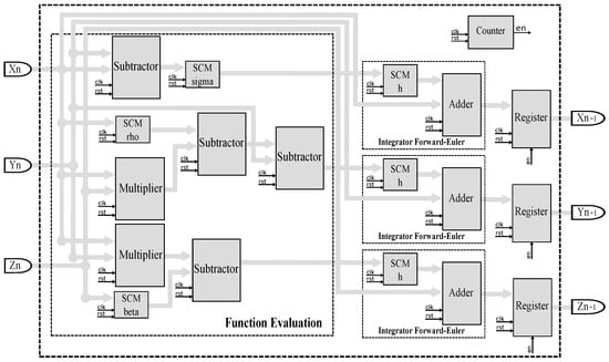
Figure 5. Block diagram of Equation (4) for field-programmable gate array (FPGA) implementation applying Forward Euler (FE).

The discretization of CO1 by applying an implicit method like Backward Euler (BE) is given in Equation (5), where it can be appreciated that the predictor is the FE given in Equation (4) to evaluate $x_{{fe}_{n+1}},x_{{fe}_{n+1}},x_{{fe}_{n+1}}$. The block description for FPGA implementation is more complex and it embeds the FE method as shown in Figure 6. One can infer that the hardware resources for the BE method almost double compared to FE.

$$\begin{array}{cc}\hfill & x_{n+1}=x_n+h\left[\sigma (y_{f{e}_{n+1}}-x_{f{e}_{n+1}})\right]\hfill \\ \hfill & y_{n+1}=y_n+h[-x_{f{e}_{n+1}}{z}_{f{e}_{n+1}}+\rho x_{f{e}_{n+1}}-y_{f{e}_{n+1}}]\hfill \\ \hfill & z_{n+1}=z_n+h[x_{f{e}_{n+1}}{y}_{f{e}_{n+1}}-\beta z_{f{e}_{n+1}}]\hfill \end{array}$$

(5)

Figure 6. Block diagram description of Equation (5) applying Backward Euler (BE) highlighting function evaluation, integrator Forward Euler and integrator Backward Euler blocks.

The application of other one-step and multi-step methods to discretize a (hyper-)chaotic oscillator is performed in a similar manner as for the FE and BE methods. For example, the application of the multi-step sixth-order Adams–Bashforth (AB6) method is more complex than FE or BE. It requires five past steps associated to $f\left(n\right),f(n-1),$$f(n-2),f(n-3),f(n-4),f(n-5)$ that can be evaluated by the 4th-order Runge–Kutta (RK4) method. In this manner, using the iterative equation associated to AB6 that is given in Table 3, the discrete equations of CO1 are given in Equation (6). Figure 7 shows the block description for the FPGA implementation of CO1. One can see the predictor RK4, function evaluation and integrator Adams–Bashforth blocks, which are designed as for the FE and BE methods. The evaluation of Equation (6) also requires a finite-state machine (FSM) to control the iterative process, a cumulative sum block to process the RK4 method and random access memories (RAMs) to save the past steps $f\left(n\right),f(n-1),f(n-2),f(n-3),f(n-4),f(n-5)$ that are required for the next iteration, and they are controlled by STP (StarT Prediction) and EOP (End Of Prediction). The predictor RK4 is disconnected after the first iteration, which is controlled by the FSM.

$$\begin{array}{cc}\hfill & x_{ab{6}_{n+1}}=x_n+h/1440[4277f\left(n\right)-7923f(n-1)+9982f(n-2)-7298f(n-3)+2877f(n-4)-475f(n-5)]\hfill \\ \hfill & y_{ab{6}_{n+1}}=y_n+h/1440[4277f\left(n\right)-7923f(n-1)+9982f(n-2)-7298f(n-3)+2877f(n-4)-475f(n-5)]\hfill \\ \hfill & z_{ab{6}_{n+1}}=z_n+h/1440[4277f\left(n\right)-7923f(n-1)+9982f(n-2)-7298f(n-3)+2877f(n-4)-475f(n-5)]\hfill \end{array}$$

(6)

Figure 7. Block diagram description of Equation (6) for FPGA implementation applying AB6 highlighting function evaluation, integrator Adams–Bashforth, cumulative sum, finite-state machine (FSM) and RK4.

In all the previous cases, the FPGA synthesis can be performed by adopting computer arithmetic of fixed-point notation, where the number of bits depends on the amplitudes of the state variables, as detailed in [7], where one can also find guidelines on Very High Speed Integrated Circuit Hardware Description Language (VHDL) programming. In this paper, the fixed-point notation has the format 12.20. Table 6 summarizes the hardware resources for the implementation of CO1, CO2, CO3, HO4 and HO5 applying FE and using FPGA Cyclone IV EP4CGX150DF31C7 under the synthesizer of software “Quartus II 13.0”. In the same table, the last two rows provide the number of clk cycles that are required to evaluate one iteration n, and the latency is given in nanoseconds when using a 50 MHz clk signal.

Table 6. Hardware resources using FPGA Cyclone IV EP4CGX150DF31C7 and applying FE to CO1, CO2, CO3, HO4 and HO5.

Resources	CO1	CO2	CO3	HO4	HO5	Available
Logic elements	1295	1083	2567	2554	1707	149,760
Registers	654	565	588	1591	1045	149,760
9*9 bit multipliers	16	8	8	135	92	720
Max freq (MHz)	90.88	102.75	58.55	79.77	82.7	50
Clock cycles by iteration	5	7	9	12	9	-
Latency (ns)	100	140	180	240	180	-

Table 7 shows the hardware resources for CO1 using FPGA Cyclone IV EP4CGX150DF31C7 under “Quartus II 13.0” and by applying the three one-step (FE, BE, RK4) and three multi-step (AB6, AM4, G4) methods. As supposed, FE requires the lowest hardware resources and clks to process one iteration. The use of SCMs makes a considerable reduction on the number of multipliers. Although RK4 requires almost four times the hardware resources than FE, it is more exact and allows a higher h [7]. AB6 requires the higher number of hardware resources compared to the other five methods. If one does not design an SCM, the VHDL description of AB6 will require more than the 720 available multipliers in the FPGA Cyclone IV, and therefore it may not be implemented on this FPGA, so that one must use an FPGA with more density resources.

Table 7. Hardware resources for CO1 using FPGA Cyclone IV and applying different methods.

Resources	FE	BE	RK4	AB6	AM4	G4	Available
Logic elements	1295	1988	4708	8512	7684	7220	149,760
Registers	654	1160	2662	4232	3856	3484	149,760
Multipliers	16	32	208	325	290	274	720
Freq (MHz)	90.88	92.59	84.77	83.53	84.18	82.73	50
Clks/iteration	5	11	32	190	130	100	-
Latency (ns)	100	220	640	3800	2600	2000	-

The hardware resources for the FPGA implementation of the remaining chaotic systems labeled as CO2, CO3, HO4 and HO5, have similar increases for each numerical method, the main difference being due to the number of ODEs and nonlinear functions.

Figure 8 shows a representative case of the FPGA implementation of CO1 applying the one-step method BE, and Figure 9 shows the application of the multi-step method G4, considering $h=0.001$ in both cases.

Figure 8. FPGA simulation of CO1 applying BE.

Figure 9. FPGA simulation of CO1 applying G4.

6. Conclusions

We have shown the issues with the FPGA implementation of chaotic and hyper-chaotic oscillators from the selection of a one-step and multi-step numerical method. The challenge is the selection of the time-step h to increase the frequency of operation of the FPGA design. It was appreciated that each one-step or multi-step method requires different hardware resources, so that trade-offs arise among reducing hardware resources, improving exactness and maximum operation frequency. Another open problem is the selection of the best chaotic oscillator, which can be done by evaluating the LE+ and $D_{KY}$. This last characteristic increases as the number of ODEs increases, so that according to the results provided by TISEAN, the hyper-chaotic oscillators have the higher LE+ and $D_{KY}$ values. The FPGA implementation of the Lorenz system CO1 showed good agreement on the time series generated by applying BE and G4 methods, and using 32 bits in fixed-point notation of 12.30. The exactness can also be accomplished through using more bits, so that one can enhance applications in chaotic secure communications and the Internet of Things (IoT) to guarantee security and privacy. In particular, the IoT application requires a connectivity protocol in which chaotic oscillators can be synchronized to mask the data being transmitted, like in the extremely lightweight publish/subscribe messaging transport known as MQTT (mqtt.org), which is ideal for connecting remote devices with a small code footprint and minimal network bandwidth.

References

- Fuchs, A. Nonlinear Dynamics in Complex Systems, 1st ed.; Springer: Berlin/Heidelberg, Germany, 2013. [Google Scholar] [CrossRef]
- Muñoz-Pacheco, J.M.; Guevara-Flores, D.K.; Félix-Beltrán, O.G.; Tlelo-Cuautle, E.; Barradas-Guevara, J.E.; Volos, C.K. Experimental Verification of Optimized Multiscroll Chaotic Oscillators Based on Irregular Saturated Functions. Complexity 2018, 2018, 3151840. [Google Scholar] [CrossRef]
- Vaidyanathan, S.; Lien, C.H.; Fuadi, W.; Mujiarto; Mamat, M.; Subiyanto. A New 4-D Multi-Stable Hyperchaotic Two-Scroll System with No-Equilibrium and its Hyperchaos Synchronization. J. Phys. Conf. Ser. 2020, 1477, 022018. [Google Scholar] [CrossRef]
- Shang, Y. Deffuant model with general opinion distributions: First impression and critical confidence bound. Complexity 2013, 19, 38–49. [Google Scholar] [CrossRef]
- Wolf, A.; Swift, J.B.; Swinney, H.L.; Vastano, J.A. Determining Lyapunov exponents from a time series. Phys. D Nonlinear Phenom. 1985, 16, 285–317. [Google Scholar] [CrossRef]
- Hegger, R.; Kantz, H.; Schreiber, T. Practical implementation of nonlinear time series methods: The TISEAN package. Chaos Interdiscip. J. Nonlinear Sci. 1999, 9, 413–435. [Google Scholar] [CrossRef] [PubMed]
- Tlelo-Cuautle, E.; Rangel-Magdaleno, J.; de la Fraga, L.G. Engineering Applications of FPGAs; Springer International Publishing: Cham, Switzerland, 2016; pp. 1–222. [Google Scholar] [CrossRef]
- Fountain, D.M.; Kolias, A.G.; Laing, R.J.; Hutchinson, P.J. The financial outcome of traumatic brain injury: A single centre study. Br. J. Neurosurg. 2017, 31, 350–355. [Google Scholar] [CrossRef] [PubMed]
- Chen, H.; Bayani, A.; Akgul, A.; Jafari, M.A.; Pham, V.T.; Wang, X.; Jafari, S. A flexible chaotic system with adjustable amplitude, largest Lyapunov exponent, and local Kaplan—Yorke dimension and its usage in engineering applications. Nonlinear Dyn. 2018, 92, 1791–1800. [Google Scholar] [CrossRef]
- Yakovleva, T.V.; Kutepov, I.E.; Karas, A.Y.; Yakovlev, N.M.; Dobriyan, V.V.; Papkova, I.V.; Zhigalov, M.V.; Saltykova, O.A.; Krysko, A.V.; Yaroshenko, T.Y.; et al. EEG Analysis in Structural Focal Epilepsy Using the Methods of Nonlinear Dynamics (Lyapunov Exponents, Lempel-Ziv Complexity, and Multiscale Entropy). Sci. World J. 2020, 2020, 8407872. [Google Scholar] [CrossRef] [PubMed]
- Akhmet, M.; Tleubergenova, M.; Zhamanshin, A. Inertial Neural Networks with Unpredictable Oscillations. Mathematics 2020, 8, 1797. [Google Scholar] [CrossRef]
- Jia, H.; Guo, C. The Application of Accurate Exponential Solution of a Differential Equation in Optimizing Stability Control of One Class of Chaotic System. Mathematics 2020, 8, 1740. [Google Scholar] [CrossRef]
- Lin, C.H.; Hu, G.H.; Yan, J.J. Chaos Suppression in Uncertain Generalized Lorenz–Stenflo Systems via a Single Rippling Controller with Input Nonlinearity. Mathematics 2020, 8, 327. [Google Scholar] [CrossRef]
- Lorenz, E.N. Deterministic nonperiodic flow. J. Atmos. Sci. 1963, 20, 130–141. [Google Scholar] [CrossRef]
- Gosar, Z. Chaotic Dynamics—Rössler System. Unpublished work. 2011. [Google Scholar] [CrossRef]
- Tlelo-Cuautle, E.; Quintas-Valles, A.D.J.; de la Fraga, L.G.; Rangel-Magdaleno, J.D.J. VHDL Descriptions for the FPGA Implementation of PWL-Function-Based Multi-Scroll Chaotic Oscillators. PLoS ONE 2016, 11, e0168300. [Google Scholar] [CrossRef] [PubMed]
- Vaidyanathan, S.; Tlelo-Cuautle, E.; Munoz-Pacheco, J.M.; Sambas, A. A new four-dimensional chaotic system with hidden attractor and its circuit design. In Proceedings of the 2018 IEEE 9th Latin American Symposium on Circuits & Systems (LASCAS), Puerto Vallarta, Mexico, 25–28 February 2018; pp. 1–4. [Google Scholar] [CrossRef]
- Chapra, S.C.; Canale, R.P. Numerical Methods for Engineers, 5th ed.; McGraw-Hill/Interamericana: New York, NY, USA, 2006. [Google Scholar]
- Tannehill, J.C.; Anderson, D.A.; Pletcher, R.H. Computational Fluid Mechanics and Heat Transfer, 2nd ed.; Taylor & Francis: Boca Raton, FL, USA, 1997; pp. 1–740. [Google Scholar]
- Sano, M.; Sawada, Y. Measurement of the Lyapunov Spectrum from a Chaotic Time Series. Phys. Rev. Lett. 1985, 55, 1082–1085. [Google Scholar] [CrossRef] [PubMed]
- Tlelo-Cuautle, E.; Pano-Azucena, A.D.; Guillén-Fernández, O.; Silva-Juárez, A. Analog/Digital Implementation of Fractional Order Chaotic Circuits and Applications; Springer: Berlin/Heidelberg, Germany, 2020. [Google Scholar]
Publisher’s Note: MDPI stays neutral with regard to jurisdictional claims in published maps and institutional affiliations. |
© 2021 by the authors. Licensee MDPI, Basel, Switzerland. This article is an open access article distributed under the terms and conditions of the Creative Commons Attribution (CC BY) license (http://creativecommons.org/licenses/by/4.0/).