A Kriging-Assisted Multi-Objective Constrained Global Optimization Method for Expensive Black-Box Functions ^†

Abstract

The kriging optimization method that can only obtain one sampling point per cycle has encountered a bottleneck in practical engineering applications. How to find a suitable optimization method to generate multiple sampling points at a time while improving the accuracy of convergence and reducing the number of expensive evaluations has been a wide concern. For this reason, a kriging-assisted multi-objective constrained global optimization (KMCGO) method has been proposed. The sample data obtained from the expensive function evaluation is first used to construct or update the kriging model in each cycle. Then, kriging-based estimated target, RMSE (root mean square error), and feasibility probability are used to form three objectives, which are optimized to generate the Pareto frontier set through multi-objective optimization. Finally, the sample data from the Pareto frontier set is further screened to obtain more promising and valuable sampling points. The test results of five benchmark functions, four design problems, and a fuel economy simulation optimization prove the effectiveness of the proposed algorithm.

1. Introduction

The application of surrogate models (i.e., metamodels or response surface models) has effectively enhanced optimization performance in many engineering design fields [1]. The surrogate models, which approximately replace the complex black-box functions, can not only express a practical problem in a simple form but also make researchers grasp characteristics of a primitive function step-by-step. Surrogate models include polynomial response surface [2], radial basis functions [3], multivariate adaptive regression spline [4], support vector regression [5], and kriging model [6]. The Bayesian statistic kriging, which offers the predictions of mean and variance at any point, is widely used.

The kriging-based EGO (efficient global optimization) method [7] and its extensions [8,9,10,11,12,13] have solved some optimization problems of expensive black-box objectives or constraints. Most of them are single-objective optimization approaches, which can only get one sampling point in per infill search loop. They are unable to realize expensive parallel evaluations. However, for the actual kriging-based single-objective black-box constrained objective optimization problem, if we can obtain l mutually independent sampling points with greater potential value in one cycle while ensuring that certain accuracy requirements are met, then the time consumption of the entire optimization process will be reduced by nearly l times under the condition that the maximum expensive times remain unchanged. This advantage is especially obvious when the black-box problem is extremely time-consuming. In this case, the following ideas may be appropriate for the kriging-based optimization. We first construct multiple optimization objectives from the kriging model parameters, then optimize these targets to generate the Pareto frontier set. Finally, expensive evaluation points with greater prospects are chosen. Therefore, kriging-assisted multi-objective optimization methods are attracted to improve the accuracy and efficiency of optimization.

Multi-objective optimization usually optimizes multiple conflicting objective functions at the same time. The optimization result can provide a Pareto optimal set [14] of equilibrium objectives. Luckily, the predicted information (mainly including estimated objectives and variances) from the kriging model can be used to directly or indirectly create some prospective optimization objectives at a low cost [15]. For this reason, Zakerifar [16] described the kriging-based multi-objective optimization method, whose test results indicate that kriging modeling can offer new opportunities to solve multi-objective problems. To reduce the computational complexity of multi-objective evolutionary optimization, a multi-objective robust spatial fuzzy clustering algorithm based on kriging and reference vector guidance [17] is proposed and successfully applied to image segmentation. The combination of cheap co-kriging and typical kriging, an efficient multi-objective evolutionary optimization method [18], is proposed in order to realize the antenna optimization design. To deal with the problem of scalability in the application of more than two objectives, an efficient kriging-based evolutionary multi-objective design optimization scheme [19] is proposed. Additionally, an adaptive optimization is carried out in iterative optimization settings to support uncertainty quantification and design optimization at the same time. In addition, a K-MOGA (kriging-assisted multi-objective genetic algorithm) [20] employed a kriging model to adaptively evaluate design points. Rajagopal and Ganguli [21] applied an improved K-MOGA in the conceptual design of UAV. Ahmed et al. [22] used a kriging-based bi-objective optimization design method and stability constraints to seek an optimal solution for hypersonic spines.

In the above optimization methods, evolutionary algorithms are mostly used to achieve multi-objective optimization based on the kriging model. However, there are few methods that can dig into the potential prediction information of kriging and be made full use of to reduce the computational cost of expensive evaluations and improve convergence accuracy. Based on the multi-objective PSO (particle swarm optimization) of crowding distance and generalized EI (expected improvement), Jie et al. [23] constructed kriging adaptively for each expensive target, and then used its nondominated solution to guide the update of particle swarm. By using the expected hypervolume improvement of the nondominated solution front and the feasibility probability of new candidates, a new infilling sampling criterion in kriging-based multi-objective constraint optimization [24] is proposed to complete optimal sampling. Li et al. [25] proposed a multi-objective optimization method that uses the approximate characteristics of adaptive kriging to transform an uncertain optimization problem into a determined multi-objective optimization problem. Combining the kriging model with PSO, a fast multi-objective optimization algorithm [26] depending on only a few exact evaluations is presented to complete the optimization of permanent magnet synchronous motors used in hybrid or electric vehicles. Rojas-Gonzalez et al. [27] reviewed the kriging-based multi-objective simulation optimization filling algorithm. It mainly introduces how to use the effective information provided by the kriging metamodel and balance global and local searches with the aid of multi-objective optimization. In addition, a multi-objective random simulation optimization algorithm [28] based on the kriging model has appeared to further improve the search efficiency. Some multi-objective robust optimization algorithms [29,30] that can be applied to uncertain environments also show that using the kriging model can get better optimization results.

To enhance the optimization property, a kriging-assisted multi-objective constrained global optimization (KMCGO) method is proposed to solve the following problem:

$$\begin{array}{l}\min f(\mathbf{x}),\hspace{1em}\mathbf{a}\le \mathbf{x}\le \mathbf{b},\hspace{1em}\mathbf{x}\in {\Re }^n\\ \hspace{1em}\hspace{1em}\hspace{1em}\mathrm{s}.\mathrm{t}. g_i(\mathbf{x})\le 0,\hspace{1em}\hspace{0.17em}i=1,\dots ,q\end{array}$$

(1)

In KMCGO, the sampled expensive experimental design data are first used to build or rebuild the kriging model, and then the model parameters of kriging are used to generate estimated objective, mean square error of prediction, and feasibility probability. Second, three objectives are optimized through the NSGA-II solver. Then, some more promising design points are chosen from the Pareto optimal front set. Finally, the test results of five benchmark functions, four design problems, and a fuel economy simulation optimization example on hydrogen energy vehicles show the effectiveness of KMCGO.

The structure of this article is mainly composed of five sections. The second section introduces the research background of this work; the third section elaborates on the construction of the three optimization objectives and the specific implementation process of the proposed method; the fourth section tests, researches, and analyzes five benchmark functions, four design problems, and an application simulation example; and finally, conclusions and further research directions are given.

2. Background

2.1. Kriging Model

For m design points, kriging based on statistical interpolation and composed of the trend function $H\mathsf{\beta }$ and random process $Z(x)$ [31] can be written as

$$y(x)=H\mathsf{\beta }+Z(x)$$

(2)

where the matrix $H$ is composed of the regression function $h_i(x^{(j)})$($i=1,\dots , p$,$j=1,\dots , m$). The vector $\mathsf{\beta }$ is formed by the coefficients of all regression functions. The function $Z(x)$ is the realization of a stochastic process with zero mean and nonnegative covariance of

$$Cov[z(x_i),z(x_j)]={\sigma }^{2}R(\mathsf{\theta },x^{(i)},x^{(j)})$$

(3)

The above parameters ${\sigma }^2$ and $\mathsf{\theta }$ are, respectively, process variance and correlation coefficient vector. For an n-dimensional problem, the spatial correlation function $R(\mathsf{\theta },x^{(i)},x^{(j)})$ that represents the correlation between point $x^{(i)}$ and point $x^{(j)}$ is shown by

$$R(\mathsf{\theta },x^{(i)},x^{(j)})={\displaystyle \prod _{k=1}^n{R}_k({\theta }_k,x_k^{(i)}-x_k^{(j)})}$$

(4)

Based on an unbiased estimator, the regression term $H\mathsf{\beta }\approx Y$ has a generalized least squares solution (Equation (4)) and maximum likelihood estimation (Equation (5)) of variance.

$$\widehat{\mathsf{\beta }}={(H^{\mathrm{T}}{R}^{-1}H)}^{-1}{H}^{\mathrm{T}}{R}^{-1}Y$$

(5)

$${\widehat{\mathsf{\sigma }}}^2=\frac{1}{m}{(Y-H\widehat{\mathsf{\beta }})}^{\mathrm{T}}{R}^{-1}(Y-H\widehat{\mathsf{\beta }})$$

(6)

The correlation matrix $R_{m\times m}$ is composed of $R(\mathsf{\theta },x^{(i)},x^{(j)})$($i,j=1,\dots , m$). The predicted objective and MSE (mean square error) for the kriging model at any point ${\mathrm{x}}^{*}$ can be expressed by Equations (6) and (7), respectively.

$$\widehat{y}(x^{*})=H\widehat{\mathsf{\beta }}+r^{\mathrm{T}}(x^{*})\widehat{\mathsf{\gamma }}$$

(7)

$${\widehat{s}}^2(x^{*})=\mathrm{MSE}[Y(x^{*})]={\widehat{\mathsf{\sigma }}}^2\left\{1-[h{(x^{*})}^{\mathrm{T}} r{(x^{*})}^{\mathrm{T}}]\left[\begin{array}{l}0 H^{\mathrm{T}}\\ H R\end{array}\right]\left[\begin{array}{l}h(x^{*})\\ r(x^{*})\end{array}\right]\right\}$$

(8)

where $\widehat{\mathsf{\gamma }}=R^{-1}(Y-H\widehat{\mathsf{\beta }})$,$r^{\mathrm{T}}(x^{*})=[R(\mathsf{\theta },x^{*},x_1^{*}),\dots ,R(\mathsf{\theta },x^{*},x_m^{*})]$.

2.2. Multi-Objective Constrained EGO Algorithm

Based on single objective optimization, the EGO [7] algorithm can use the prediction objective $\widehat{y}$ and standard deviation $\widehat{s}$ of the kriging model to construct the infill sampling criterion EI shown in Equation (8).

$$EI(x)=\left\{\begin{array}{ll}(f_{\min }-\widehat{y})\Phi (\frac{f_{\min }-\widehat{y}}{\widehat{s}})+s\varphi (\frac{f_{\min }-\widehat{y}}{\widehat{s}})& \mathrm{if} \widehat{s}>0\\ 0& \mathrm{if} \widehat{s}=0\end{array}\right.$$

(9)

In Equation (8), the expresses $\Phi (\cdot )$ and $\varphi (\cdot )$ are the normal cumulative distribution function and probability density function, respectively. The sign $f_{\min }$ is the minimum value of the existing expensive objective evaluations. The EGO first creates kriging approximation by performing initial sampling and expensive function estimation, and then EI is maximized to get new update points. This process will continue to loop until termination conditions are met.

When the distance between an unsampled point and the current optimal solution is far, big EI can effectively balance exploration and exploitation for kriging. However, in some cases, EGO is easy to sink into the local optimal basin when the optimal solution has been found in initial sampling. In addition to this, the introduction of sampling points will lead to the increasing cost of calculation. How to overcome these difficulties needs to be studied in depth.

The constraints based on the kriging model are mainly realized by two methods. One is to calculate the feasibility probability (PF) of constraint functions. Another way is to take the expectation violation (EV) as the constraint condition and obtain the feasible solutions in the iterative optimization process.

The expression [32] on the EV is shown in Equation (9). The EV is similar to the EI. When constraints are not violated or show big uncertainty, the EV has a high reference value. If the value is higher than the specified threshold, it is generally considered that the current sampling point is feasible. Maximizing the PF of constraints [33] has attracted more researchers’ attention. Due to the estimated mean ${\widehat{g}}_i(x)$ and root mean square error (RMSE) ${\widehat{s}}_{g_i}(x)$ of the ith constraint, the corresponding PF is shown in Equation (10).

$$E{V}_i(x)=-{\widehat{g}}_i(x)\Phi \left(-\frac{{\widehat{g}}_i(x)}{{\widehat{s}}_{g_i}(x)}\right)+{\widehat{s}}_{g_i}(x)\Phi \left(-\frac{{\widehat{g}}_i(x)}{{\widehat{s}}_{g_i}(x)}\right)$$

(10)

$$P{F}_i(\mathrm{x})=\Phi \left(-\frac{{\widehat{g}}_i(\mathrm{x})}{{\widehat{s}}_{g_i}(\mathrm{x})}\right)$$

(11)

By multiplying the EI and PF ($EI\times PF=EI\times {\displaystyle \prod _{i=1}^{q}P{F}_i}$) [34], a constrained optimization problem can be transformed into an unconstrained one.

3. KMCGO Method

For kriging-based multi-objective optimization, the combination of kriging prediction objective and estimation variance can be maximized in the sampling optimization process to achieve a balance between global and local searches to a certain extent. In addition, to prevent the construction failure resulting from the singularity of the covariance matrix R in the kriging modeling process, it is necessary to avoid any two sampling points being too close. Further, selecting a more promising sampling point from the Pareto frontier set can reduce many unnecessary expensive function evaluations, which is also in line with the original intention of surrogate model optimization. If these factors are taken into consideration to realize the constraint optimization based on the kriging model, the convergence accuracy might be further improved. In view of this condition, three objectives introduced into KMCGO are optimized to further select update points and complete the exploration of the optimal feasible solution.

3.1. Three Optimization Objectives

3.1.1. Optimization Objective I

The constrained optimization based on the kriging model not only requires that an algorithm has a more careful search in local region near the optimal solution, but also hopes that it can dig out some more promising sampling points from some unexplored areas. To this end, it need take advantage of some parameters of the known kriging model.

For the kriging model, when two points are farther apart, they have a higher mutual independence, and their correlation is close to 0, which can ensure that the information of the two points is mutually exclusive. It can ensure that each point has the greatest value to the model construction. Similarly, when the two points are closer together, the mutual independence between the two sampling points is lower, and the correlation value is closer to 1. This easily causes the correlation matrix R of the kriging model to be not full rank and become ill-conditioned, which in turn results in the update of the kriging model to fail. Therefore, it is necessary to ensure that the distance between the acquired sample point and the existing sample is not too close by a certain method. To avoid this issue, Equation (11) can be employed to describe the first optimization objective:

$$\min \widehat{f}(x)\cdot d^e, \mathrm{s}.\mathrm{t}. a\le x\le b$$

(12)

where parameter $\widehat{f}(x)$ is the prediction of the kriging model at any point $\mathrm{x}$. The non-negative weight index e is polled in a set of increasing number sequence $\{e_1,e_2\dots ,e_k\}$ greater than or equal to 0 to adjust the influence of the distance factor $d$ in the objective function according to iteration times. The recommended choice in this work is a geometric sequence as shown in $\{\dots ,0.001,0.01,0.1,1,10,\dots \}$. The adaptive choice of e in the iteration process can be described as follows: We assume that the iteration number is $iternum$. When $\mathrm{mod}(iternum,k)\ne 0$ is satisfied, the current value of e is set to $e_{\mathrm{mod}(iternum,k)}$. Otherwise, it is assigned to $e_k$. In addition, the distance factor $d$ [35] is shown in Equation (12).

$$d=\left\{\begin{array}{c}1-\frac{d_{\max }-d_{\min }^{’}}{\left|\right|b-a\left|\right|},\widehat{f}(x)\le 0\\ \frac{d_{\max }-d_{\min }^{’}}{\left|\right|b-a\left|\right|},\widehat{f}(x)>0\end{array}\right.$$

(13)

In Equation (12), the parameter $d_{\max }$ is a maximum distance between all existing sampled design points $(x_1,...,x_m)$. The parameter $d_{\min }^{’}=\min (||x-x_1||,\dots ,||x-x_m||)$ is the minimal distance value between a candidate point $\mathrm{x}$ and any point of the set $\mathrm{X}={[x_1,...,x_m]}^{\mathrm{T}}$.

3.1.2. Optimization Objective II

If the candidate points generated by kriging-based optimization lie on the boundary of the approximate constrained model, they may not be the real feasible sampling points. However, the candidate points near the feasible region with a small deviation from the constraint boundary may be the real feasible points.

When the values of all constraint functions in problem (1) are less than or equal to zero, the corresponding sampling point is considered feasible. However, the calculation is a little cumbersome. For this reason, we set a maximum constraint violation as the equation $g_{\max }=\max [g_1(x),\dots ,g_q(x)]$. If this violation $g_{\max }$ is not greater than 0, we believe that other constraints are also satisfied. When all constraint functions in KMCGO are replaced by kriging models, the probability of maximum constraint violation [11] is expressed by

$$P(g_{\max }\le 0)=1-\Phi ({\widehat{g}}_{\max }/{\widehat{s}}_{\max })$$

(14)

where the sign $\Phi (\cdot )$ is a normal cumulative distribution function, and the value of ${\widehat{s}}_{\max }$ can be calculated by Formula (7). As Equation (14) shows, a sampling point with great feasibility can be obtained by maximizing the feasible probability P.

$$\begin{array}{l}\max P\\ \mathrm{s}.\mathrm{t}. a\le x\le b\end{array}$$

(15)

3.1.3. Optimization Objective III

For the objective function and constraint function approximated by the kriging model, it is necessary to consider the RMSE (see Equation (7)) predicted by kriging in the KMCGO method. For the kriging approximate function, large estimated RMSE is helpful for KMCGO to explore some undeveloped regions so as to further enhance the possibility of obtaining the global optimal solution. Furthermore, the application of maximizing RMSE and minimizing problem (11) is conductive to balance exploration and exploitation. Therefore, in the KMCGO optimization process, it is appropriate to use the kriging model to approximate the objective function and maximize its RMSE.

Besides the objective function, the estimated RMSEs for constraint functions should also be taken into account. Assuming that a global optimal solution is located in the region with large prediction variance, KMCGO may be unable to seek out the optimal solution with sufficient credibility in the optimization process. Thus, reducing the RMSE of an effective constraint will be used to explore an approximate global optimal solution close to the actual constraint boundary. Therefore, minimizing the predicted RMSEs of constraints is feasible in the whole process of KMCGO optimization. To this end, the third optimization objective is defined as Equation (15).

$$\max \left[{\widehat{s}}_f(x)-{\displaystyle \sum _{i=1}^q{\widehat{s}}_{g_i}(x)}\right]$$

(16)

All estimates of the root mean square error in Equation (15) can be calculated by Equation (7).

Finally, the three optimization objectives are gathered together and shown in Equation (16) according to Section 3.1.1, Section 3.1.2 and Section 3.1.3.

$$\left\{\min \widehat{f}(x)\cdot d^e, \min [-P], \min \left[{\displaystyle \sum _{i=1}^q{\widehat{s}}_{g_i}(x)}-{\widehat{s}}_f(x)\right]\right\}$$

(17)

3.2. Deep Filtering of Data in Pareto Optimal Set

Using the NSGA-II solver to optimize the three objectives in Formula (16) can generate the Pareto frontier. Because there are many sampling points in the Pareto frontier, they cannot all meet the requirements of being good feasible points. Therefore, it is very important to design an effective filtering method to select more promising candidates from the Pareto optimal frontier. It is assumed that the Pareto frontier set is ${\mathrm{X}}^{’}=\{{\mathrm{x}}_1,\dots ,{\mathrm{x}}_j\}$. After the set ${\mathrm{X}}^{’}$ and the sampled sample set $\mathrm{X}$ are standardized, we will follow the steps below to complete the deep filtering of the Pareto frontier data [36].

Step 1: For any candidate point $x_i$ in the Pareto frontier set, if the feasible probability (see Formula (13)) is not less than 99%, we believe that such sampling point is feasible and can be temporarily accepted. When the number $v$ of the accepted sampling points is not less than 4n, it will skip to step 3. Otherwise, it need carry out step 2 in sequence. The reasons can be explained as follows.

First, obtaining feasible sampling points is the premise and foundation for further constraint optimization. Multi-objective optimization focuses on the mutual balance between optimization objectives. However, it does not consider the feasibility of sampling points. If it has been unable to obtain any feasible point, then it is impossible to explore the feasible optimal solution, and the next optimization will be meaningless. Therefore, the optimization of objective 2 in Formula (14) is a prerequisite for obtaining feasible sampling points and sample selection. Therefore, it is essential to satisfy the condition $P\left(g_{\max }(x_i)\le 0\right)\ge 99\%$ here.

Step 2: If there are no such candidates, the $w$ sampling points, whose feasible probability is close to 99%, will be chosen to perform further filtering. It should be noted that the number $v$ of sampling points with feasible probability greater than 99% and the number w of sampling points with feasible probability close to 99% should be equal to 4n.

Step 3: When the distance between the new sampling point and the existing sampling data is too close, it may lead to the failure of kriging construction. To avoid this, it should first calculate the minimum distance $d_{\min }=\left|\right|x_m-x_n|{|}^2, m\ne n$ in the sample set $\mathrm{X}$. Another minimum distance $d_{\min }^{’}=\left|\right|x_i-x_k|{|}^2$($x_k\in \mathrm{X}$) between the new choice point $x_k$ ($k\in 1,\dots ,j$) and $\mathrm{X}$ should also be calculated. Due to $d_{\min }$ and $d_{\min }^{’}$, the distance improvement index $\delta =|y_m-y_n|/d_{\min }$ in the set $\mathrm{X}$ and the new distance improvement index ${\delta }^{’}=|{\widehat{y}}_i-y_k|/d_{\min }^{’}$ of an update point can be generated. When ${\delta }^{’}<\delta$, $x_k$ will be abandoned, or else, the point $x_i$ will be accepted.

Step 4: In order to balance the local and global search behaviors, the new sampling point with a larger estimated variance and a smaller predicted objective is appropriate. Therefore, for each newly selected candidate point, we subtract the predicted RMSE (see Equation (7)) from the estimated objective (see Equation (6)), and the results are arranged in the order of small to large. Finally, the sampling points corresponding to the 2*n data arranged in the front are selected as the final sample points for expensive evaluations.

3.3. Exploration of Promising Areas

In KMCGO, how to jump out of the current local optimal area is a problem that needs to be dealt with. If no better feasible point is discovered after 2*n+1 function evaluations, and the number $k$ of the feasible sampling points $\{x_1,\dots ,x_k\}$ newly selected is not less than 2*n, it is considered that the current optimization region may not be suitable for further search. In that way, the KMCGO algorithm should jump out of the current basin and search for some promising solutions to other unexplored areas. Even if the number $k$ is less than 2*n or equal to 0, it is also reasonable to jump out of the current area and explore more promising areas. For this, we use the point $x^{*}=(x^{*}\left(1\right), x^{*}\left(2\right))\leftarrow (x_1+\cdot \cdot \cdot +x_k)/2$ as a center one, and increase or decrease the value $d_{\mathrm{mean}}$ = $(d_{\max }-d_{\min })/2$ for each coordinate axis to generate 2ⁿ+1 new points. Like in a two-dimensional problem, all new points are $(x^{*}\left(1\right), x^{*}\left(2\right))$,$(x^{*}\left(1\right)\pm d_{\mathrm{mean}}, x^{*}\left(2\right))$, and $(x^{*}\left(1\right), x^{*}\left(2\right)\pm d_{\mathrm{mean}})$, respectively. If $x^{*}\left(1\right)-d_{\mathrm{mean}}$ is lower than $a(1)$, we will use $a(1)$ instead of $x^{*}\left(1\right)-d_{\mathrm{mean}}$. Other situations are similar to it. Then a final sampling point $x_{\mathrm{final}}$ with good feasibility and small objective estimation value is chosen from the four new points. At the same time, the function evaluation of $x_{\mathrm{final}}$ is carried out, and it is added to the sample set $\{X,Y\}$ to rebuild the kriging model and perform the next iterative optimization.

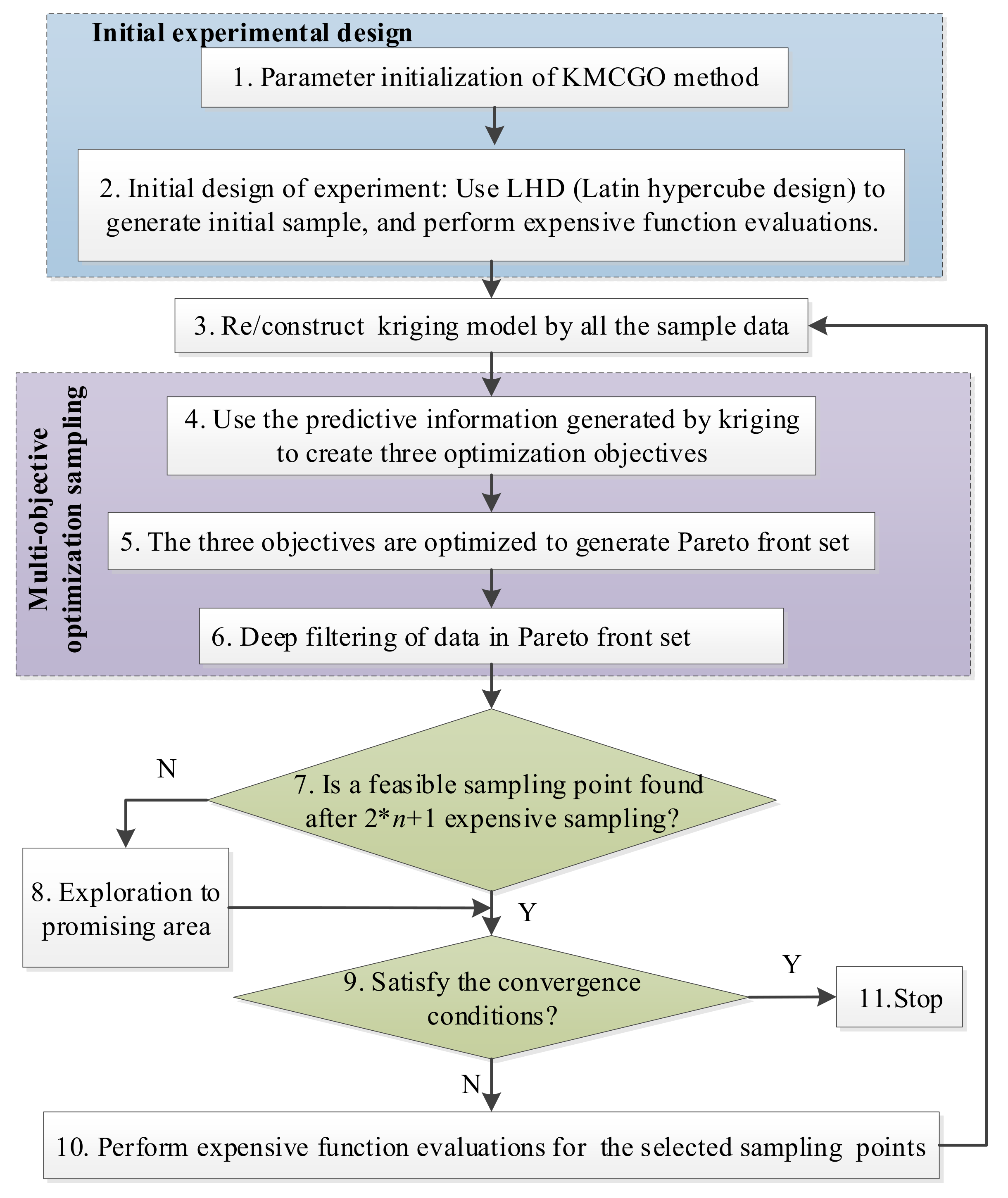
3.4. The Specific Implementation Flows

The flowchart and specific realization are shown in Figure 1. The input and output of KMCGO are shown in

Table 1. Input and output parameters of the KMCGO method.

Input

A black-box problem $f(x)$ and constrain functions $g_1(x),\dots ,g_q(x)$. Initial sampling data $X={[x_1,\dots ,x_{\mathrm{m}}]}^{\mathrm{T}}$ obtained by LHD (Latin hypercube design) [37]. A kriging model using Gaussian correlation expression as kernel function. Set the upper limit value $N_{\max }$ of expensive evaluation number as $20*n+10$. The non-negative exponential parameter e will be adaptively selected from the data set $\{0.0001,0.001,0.01,0.1,1,10,100\}$.

Output

The optimal point $(x_{\mathrm{best}},y_{\mathrm{best}})$ obtained by KMCGO.

and

Table 2. The specific realization of the KMCGO method.

The KMCGO Method

Step 1.Parameter initialization. For different optimization problems, the initial parameters (for example, design domain, number of initial sampling points, some parameters given in Table 1, etc.) of the kriging model are assigned. Step 2. Initial experiment design. In order to be able to search for more unknown areas, thereby increasing the probability of obtaining feasible sampling points, it is necessary to slightly increase some initial experimental design points. Therefore, for the n-dimensional problem, 2*n+6 initial sampling points are obtained by LHD. Next, the expensive function evaluation is carried out for each sampling point to form the initial sample set $\{X,Y\}$. Finally, the initial sample set is divided into feasible sample set $\left\{X_{\mathrm{fea}},Y_{\mathrm{fea}}\right\}$ and infeasible one $\left\{X_{\mathrm{infea}},Y_{\mathrm{infea}}\right\}$ by calculating and judging the values of all constraint functions. Meanwhile, the initial optimal solution is assigned as $(x_{\mathrm{best}},y_{\mathrm{best}})$. Step 3. Re/constructing kriging. Use the current sample set $\{X,Y\}$ ($\{X,Y\}$ = $\left\{X_{\mathrm{fea}},Y_{\mathrm{fea}}\right\}$+$\left\{X_{\mathrm{infea}},Y_{\mathrm{infea}}\right\}$) to construct the kriging surrogate model of objective and constraint functions. Step 4. Creating three optimization objectives. The prediction parameter $\widehat{f}$, ${\widehat{g}}_i$ and RMSE related to the objective and constraints can be calculated by the kriging model (see Equations (8) and (9)). The three optimization objectives in Equation (16) will be formed by the prediction parameters. Refer to Section 3.1 for the specific construction process. Step 5. Optimizing three objectives. The three objectives generated in Step 4 are optimized by the NSGA-II solver to generate the Pareto frontier. Step 6. Deep filtering of data in the Pareto frontier set. The data in the Pareto frontier need further judgment and detection, and select promising sampling points for expensive black-box evaluations. Section 3.2 details the selection process. Step 7. Determining whether a feasible point has been found. When some feasible sampling point(s) can be found after 2*n+1 expensive function evaluations, it needs to skip to Step 9 directly. Otherwise, Step 8 will be executed in sequence. Step 8. Exploration on more promising areas. See Section 3.3 for the specific process. Step 9. Stop criterion. Determine whether the given stop criterion is met. If not, perform Step 10 in sequence. Otherwise, skip to Step 11. Step 10. Expensive evaluations of new selected sampling points. The new sampling points finally selected from the above steps will be used for expensive function evaluations. Additionally, the sampling points and evaluation results will be classified and respectively added to the sample sets $\{X_{\mathrm{fea}},Y_{\mathrm{fea}}\}$ and $\{X_{\mathrm{infea}},Y_{\mathrm{infea}}\}$. Step 11. Stop. The whole iterative process is finished, and the global optimal solution $(x_{\mathrm{best}},y_{\mathrm{best}})$ is the output.

.

4. Test

To verify the performance of the proposed method, five benchmark numerical functions [38] (G4, G6, G7, G8, and G9) and four design problems (TSD-tension string design, PVD-pressure vessel design, WBD-welded beam design, SRD-speed reducer design) [39] were tested. Among them, the main information is shown in

Table 3. The main information of test problems. It includes BDF (benchmark or design problems), D (dimension), NCF (number of constraint functions), bound constraint, GOS (global optimal solution), and RET (relative error threshold).

BDF	D	NCF	Bound Constraint	GOS	RET
G8	2	2	[0, 10]2	−0.095825	1 × 10−4
G6	2	2	[13, 100] × [0, 100]	−6961.81388	1 × 10−5
TSD	3	4	[0, 100]3	0.01267	0.05
PVD	4	4	[0.0625, 6.1875]2 × [10, 200]2	5888.66	0.05
WBD	4	6	[0.125, 10] × [0.1, 10]3	1.7249	0.05
G4	5	6	[78, 102] × [33, 45] × [27, 45]3	−30,665.539	1 × 10−5
G9	7	4	[−10, 10]7	680.630057	0.5
SRD	7	11	[2.6, 3.6] × [0.7, 0.8] × [17, 28] × [7.3, 8.3]2 × [2.9, 3.9] × [5, 5.5]	2994.42	0.001
G7	10	8	[−10, 10]10	24.30621	0.01

.

For kriging-based constraint optimization, the KCGO (kriging-based constrained global optimization) algorithm [11] can deal with the problem that the objective and constraints are black-box functions when all sampling points are infeasible. Combined with a space reduction strategy, the SCGOSR (surrogate-based constrained global optimization using space reduction) algorithm [40] also completes the optimization of the black-box constraint problem. In addition, based on the EI, feasibility probability, and prediction variance of the constraint function, the three-objective kriging-based constrained global optimization (TOKCGO) [41] method is realized. Therefore, it first provides the iterative process of the proposed method and compares the test results with those of KCGO, TOKCOGO, and SCGOSR in this section. In the test process, KMCGO mainly uses two stop conditions: (1) For the n-dimensional test problem, except G4, set the maximum number of expensive evaluations to 50 * (n − 1); (2) calculate the relative error between the approximate optimal feasible solution and the known optimal solution, and compare it with the relative error threshold in Table 3. If the relative error calculated is not greater than the error threshold, the algorithm running process will end. Once one of the above two stop conditions is satisfied, the optimization process will be terminated. In order to facilitate the graph visualization, when the relative error of the iteration points meets the requirements but the number of all the current sampling points is not an integer multiple of 50, we take the 50*i (i is a positive integer) sampling points closest to the total sample number as the stop condition. In addition, the optimization of the fuel economy simulation for hydrogen energy vehicles in Section 4.2 also shows the practicability of the proposed method. All test questions will be executed in the software Matlab 2017b on a Dell machine equipped with i7-4790 3.6 GHz CPU and 16 GB RAM.

4.1. Numerical Test

To illustrate the features of KMCGO in detail, Figure 2 shows the first-iteration Pareto frontier of the G8 problem. The Pareto frontier formed by objectives 1 ($\widehat{f}(x)\cdot d^e$) and 3 (${\displaystyle \sum _{i=1}^q{\widehat{s}}_{g_i}(x)}-{\widehat{s}}_f(x)$) has a good trend, because the constraint problem does not play a decisive role. Due to the constraint of objective 2 ($-P$), the Pareto frontier formed by objectives 1 and 2 has certain regional discontinuity and irregularity. In the whole iterative process, two feasible sampling points with very close distance are found, and the relative error between the global approximate optimal solution searched in the iterative process and the actual optimal feasible solution is about 0.063, which shows that KMCGO has certain convergence and effectiveness to some extent.

The test results of the G8 problem are shown in Figure 3 and Figure 4. Figure 3 shows the distribution of the initial LHD sampling points and the sampling points generated in the optimization process. Figure 4 shows the iteration results of the objective function values corresponding to the expensive evaluation points (also including the initial sampling points). These figures show that optimization objective 2 in Section 3.1 makes many sampling points gather near the constraint boundary, which will further increase the probability of obtaining feasible sampling points in the next optimization sampling. In addition, optimization objectives 1 and 3 in Section 3.1 and the deep filtering method in Section 3.2 not only enables the KMCGO algorithm to search more carefully in the feasible region after finding the feasible points, but also can explore more potential feasible sampling points from the Pareto frontier. The iteration result also proves that the sampling points in the feasible region can seek some better solutions in the next optimization process. Finally, the KMCGO method has found a feasible sampling point that meets the requirements of the relative error threshold through 34 iterations. Therefore, this method is suitable for solving constrained global optimization problems such as G8.

Furthermore, KMCGO will also complete the testing of other functions except G8. The results are shown in Figure 5, Figure 6, Figure 7, Figure 8, Figure 9, Figure 10, Figure 11 and Figure 12. For G6 (Figure 5) with a narrow feasible region, although no feasible sampling point is obtained in the initial sampling, it will quickly converge to a global approximate optimal solution satisfying the requirements once a feasible sampling point is found. 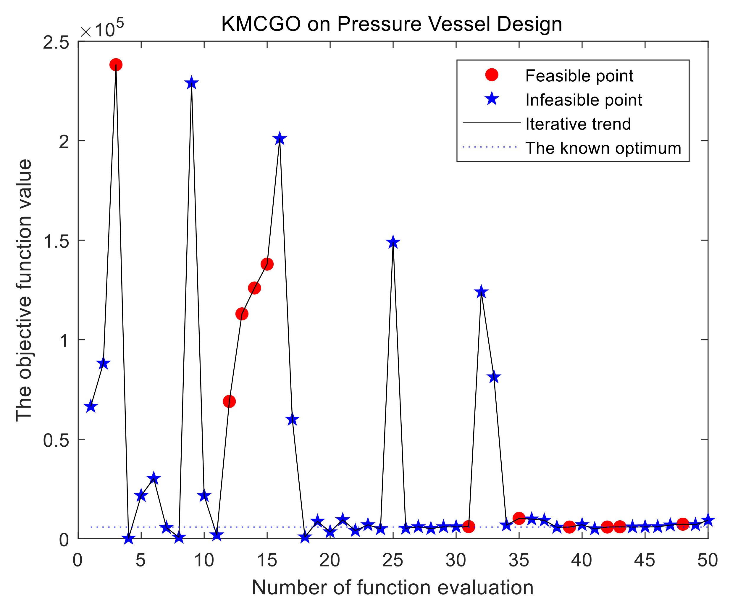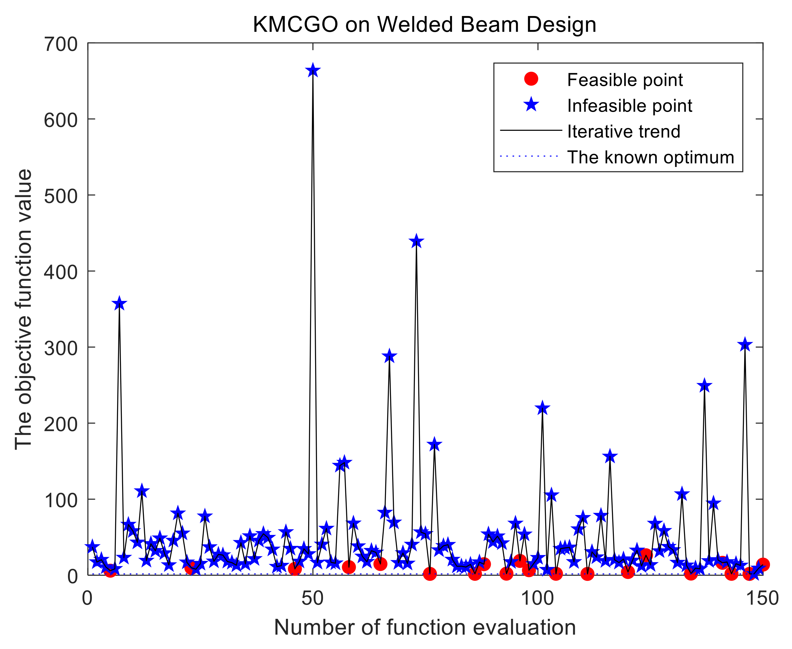For test problems such as TSD (Figure 6), PVD (Figure 7), WBD (Figure 8), and the G4 function (Figure 9) that are no more than five dimensions, as long as the feasible range is not too narrow, initial LHD sampling can find some feasible point(s) on most occasions.

For seven-dimensional problems such as the G9 function (Figure 10), SRD (Figure 11), and G7 function (Figure 12), KMCGO is unable to directly obtain feasible sampling points in the initial experimental design and usually finds feasible points in the iterative process. Therefore, it is necessary to find a better global optimal solution that satisfies the given conditions through a certain amount of evaluations. And test result of the SRD problem has good convergence, stability, and effectiveness. For example, in the 10-dimensional G7 function, it cannot obtain feasible points in the initial sampling stage because of its high dimension. In the feasible region formed by active constraints g1, g2, g3, g4, g5, and g6, the global approximate optimal solution can be found only by 150 iteration points.

To enhance the readability of the iteration test, more distinct results are given in some cases, such as TSD (Figure 6), G9 (Figure 10), and G7 (Figure 12). Obviously, KMCGO can find the appropriate approximate optimal solution, even closer to the global optimal value.

Therefore, the optimization results of the KMCGO method can meet the given accuracy requirements within the given maximum number of expensive estimates. It is suitable for black-box constrained optimization.

Refer to

Table 4. Comparison of the KMCGO, SCGOSR, TOKCGO, and KCGO methods. The comparison parameters include MEEN (mean expensive evaluation number), AOA (approximate optimum area), and RRE (real relative error).

TF	Dim	Method	MEEN	AOA	Distance to Minimizer	RRE
G8	2	KMCGO	46.2	−0.0958 ± 0.000024	[1 × 10−6, 0.000049]	[1.0 × 10−5, 5.1 × 10−4]
		SCRGOSR	51.8	−0.0958 ± 0.000013	[12 × 10−6, 0.000038]	[1.2 × 10−5, 4.0 × 10−4]
		TOKCGO	45.9	−0.0958 ± 0.000021	[4 × 10−6, 0.000046]	[4.2 × 10−5, 4.8 × 10−4]
		KCGO	47.4	−0.0958 ± 0.000020	[5 × 10−6, 0.000045]	[5.2 × 10−5, 4.7 × 10−4]
G6	2	KMCGO	41.8	−6961.802 ± 0.011	[0.00880, 0.02288]	[1.3 × 10−6, 3.3 × 10−6]
		SCRGOSR	75.1	−6961.793 ± 0.016	[0.00488, 0.03688]	[7.0 × 10−7, 5.3 × 10−6]
		TOKCGO	41.9	−6961.798 ± 0.014	[0.00188, 0.02988]	[2.7 × 10−7, 5.3 × 10−6]
		KCGO	43.6	−6961.801 ± 0.012	[0.00088, 0.02488]	[1.0 × 10−5, 4.3 × 10−6]
TSD	2	KMCGO	45.6	0.012701 ± 0.000021	[1 × 10−6, 0.000052]	[7.9 × 10−4, 4.1 × 10−2]
		SCRGOSR	75.7	0.012675 ± 0.000045	[4 × 10−6, 0.000015]	[3.2 × 10−3, 1.2 × 10−2]
		TOKCGO	44.1	0.012693 ± 0.000020	[3 × 10−6, 0.000043]	[2.4 × 10−3, 3.4 × 10−2]
		KCGO	40.8	0.012704 ± 0.000028	[6 × 10−6, 0.000062]	[4.7 × 10−3, 4.9 × 10−2]
PVD	4	KMCGO	38.8	5847.52 ± 40.31	[3.24, 83.38]	[5.6 × 10−4, 1.4 × 10−2]
		SCRGOSR	43.7	5907.2 ± 21.9	[80.85, 178.65]	[1.4 × 10−2, 3.1 × 10−2]
		TOKCGO	39.5	5903.86 ± 97.33	[6, 196.75]	[2.1 × 10−3, 3.4 × 10−3]
		KCGO	45.3	5835.81 ± 28.46	[2.9, 59.82]	[1.0 × 10−3 1.0 × 10−2]
WBD	4	KMCGO	98.4	1.7665 ± 0.026	[0.016, 0.0675]	[9.2 × 10−3, 3.9 × 10−2]
		SCRGOSR	101.9	1.7589 ± 0.032	[0.0019, 0.066]	[1.1 × 10−3, 3.8 × 10−2]
		TOKCGO	100.2	1.7834 ± 0.045	[0.0134, 0.1034]	[7.8 × 10−3, 6.0 × 10−2]
		KCGO	123.1	1.9947 ± 0.1587	[0.1110, 0.4284]	[6.4 × 10−2, 0.248]
G4	5	KMCGO	44.6	−30,665.472 ± 0.052	[0.015, 0.119]	[4.9 × 10−7, 3.9 × 10−6]
		SCRGOSR	53.9	−30,665.463 ± 0.064	[0.012, 0.140]	[3.9 × 10−7, 4.6 × 10−6]
		TOKCGO	46.5	−30,665.475 ± 0.043	[0.021, 0.127]	[6.8 × 10−7, 4.1 × 10−6]
		KCGO	32.7	−30,665.480 ± 0.035	[0.024, 0.094]	[7.8 × 10−7, 3.1 × 10−6]
G9	7	KMCGO	112.8	827.678 ± 85.57	[61.48, 255.15]	[0.0903, 0.3418]
		SCRGOSR	115.6	904.08 ± 77.78	[140.42, 294.98]	[0.2044, 0.4294]
		TOKCGO	124.4	839.195 ± 96.59	[61.98, 255.15]	[0.0916, 0.3749]
		KCGO	165.9	910.49 ± 67.96	[155.64, 291.56]	[0.2266, 0.4245]
SRD	7	KMCGO	77.3	2995.36 ± 0.95	[0.01, 1.89]	[3.34 × 10−6, 6.31 × 10−4]
		SCRGOSR	88.1	2996.15 ± 1.65	[0.08, 3.38]	[2.68 × 10−5, 1.13 × 10−3]
		TOKCGO	79.6	2996.25 ± 1.07	[0.76, 2.90]	[2.54 × 10−4, 9.68 × 10−4]
		KCGO	51.5	2997.52 ± 0.024	[3.076, 3.124]	[1.02 × 10−3, 1.04 × 10−3]
G7	10	KMCGO	124.8	24.5046 ± 0.192	[0.00639, 0.1984]	[2.63 × 10−4, 8.16 × 10−3]
		SCRGOSR	178.2	24.6559 ± 0.314	[0.00869, 0.69069]	[3.58 × 10−4, 0.02842]
		TOKCGO	130.1	24.5878 ± 0.266	[0.01559, 0.54759]	[6.41 × 10−4, 0.02253]
		KCGO	136.5	24.3139 ± 0.046	[0.00309, 0.01239]	[1.27 × 10−4, 5.10 × 10−4]

for the comparison of the KMCGO, SCGOSR, TOKCGO, and KCGO methods. For each test problem, in many cases, the average of the expensive evaluations in the KMCGO method is smaller than that of the other three optimization algorithms. This is especially evident in the PVB, WBD, G9, and G7 problems. For some problems with a narrow feasible interval (such as G6), the KMCGO and TOKCOGO methods have a smaller approximate optimal interval, while SCRGOSR and KCGO have a larger approximate optimal interval. For the problem with a wide feasible interval (such as PVD), the opposite is true. In problems on interval distance from the actual optimal solution, the KMCGO method has a smaller lower bound in many cases, which indicates that it has a greater possibility to find a smaller global optimal solution. Therefore, it can reflect the better convergence of the proposed method to a certain extent. In addition, the KMCGO method provides a better convergence effect and smaller relative error range due to the approximate optimal solution and global minimum value. Therefore, the above analysis reflects that the proposed method has good stability, feasibility, convergence, and effectiveness from different aspects. In addition, the three methods compared have their own characteristics. They also show some good performances in some test functions. For example, the KCGO and TOKCGO methods use less mean expensive evaluation number (MEEN) in the TSD and G6 problems, respectively, but their final accuracy and convergence are slightly worse. According to “distance to minimizer” and “RRE,” SCGOSR also shows good convergence in the WBD problem, but it requires a little more MEEN. However, judging from the overall performance, the proposed method shows the best performances.

For the total computational cost including the evaluation of the black-box function, if purely from the perspective of the benchmark functions, the proposed method will require a slightly higher time cost. However, the original intention of optimization based on kriging is to solve the expensive and complicated black-box problem with as few expensive valuations as possible. And its computational time consumption is usually much higher than that of kriging modeling optimization. When we apply the proposed method to the complex simulation model shown in Section 4.2, the total computational cost of all the compared optimization algorithms is almost equal. In this case, the superiority of the KMCGO method with better optimization accuracy stands out.

4.2. Fuel Economy Optimization for HFCV

The hydrogen fuel cell vehicle (HFCV) has low noise and high energy conversion efficiency. The energy generated after hydrogen fuel combustion is taken to the generator to generate electric energy and then transmitted to the vehicle battery. And then it is transmitted to the driving motor through the electric energy of the vehicle battery, thus forming the kinetic energy of vehicle movement. In the whole transmission process, the optimization of the parameters used for energy control can realize the reasonable distribution of energy between the battery and the drive motor. In view of this, the minimum power, charging power, maximum power, and minimum shutdown time of the fuel cell are taken as control strategy parameters (i.e., design variable parameters). In addition, the battery charging state, acceleration performance, speed, and climbing performance are taken as constraints. Finally, the above control strategy parameters of the hydrogen fuel cell vehicle are optimized on the advisor platform to improve the hydrogen fuel economy. The established simulation model of the vehicle system based on the hydrogen fuel cell is shown in Figure 13, and its corresponding expression of the optimization problem [42] is shown in Equation (17). According to the defined design variables, the established simulation model, and the used simulation platform, the acceleration, climbing ability, battery constraint state, and hydrogen economy of the fuel cell vehicle can be calculated by using the “adv_no_gui” function in MATLAB. In addition, the simulation of the “test procedure” function can obtain the speed error, the condition of the battery constraint state, and the hydrogen economy. Furthermore, through the “grade_test” and “accel_test” function simulation, the constraints required to limit the climbing and acceleration can be generated, respectively.

$$\max Y(x)=Hydrogen\_economy(X)$$

(18)

In order to use the proposed method for simulation optimization, the loop standard “Test_City_HYW” is set as the necessary condition of the simulation model loop. Through the initial experimental design, 20 expensive simulation evaluation points are obtained so that the initial kriging established by these 20 points can better approximate the HFCV simulation model to a certain extent. In addition, set the total number of simulation times to 100, and set 0.0001 as tolerance threshold of the active constraint function. Other design or constraint parameters not involved will maintain the settings given by the simulation system itself. Finally, the initial empirical design parameter [5 × 10³, 5 × 10³, 4.5 × 10⁴, 65] is selected as the initial model parameter value.

The objective function and constraints of the HFCV simulation model are considered to be expensive black box, so the sampling points obtained by the initial experimental design (i.e., before sequential optimization simulation) are basically not feasible. Fortunately, the KMCGO method does not need feasible sampling points in the initial samples. This kind of adaptive algorithm is also conducive to researchers’ in-depth understanding and grasp of the simulation model. In the iterative optimization process, the “adv_no_gui” function returns the hydrogen economy to the user, and the returned value is equivalent to the MPGGE (miles per gallon gasoline equivalent). Therefore, it uses MPGGE as objective and finishes the simulation optimization by maximizing this objective.

None of the 20 sampling points designed in the initial experiment is feasible. The MPGGE with the least constraint conflict is 61.0891. In view of this, the KMCGO method needs to find a feasible point after initial sampling. Additionally, before the termination condition is satisfied, the optimal feasible solution needs to be found. Through acceleration test, climbing test, simulation test, and 100 expensive simulation estimates under cyclic conditions, the time spent is about 40 h.

The flowchart and specific realization are respectively shown in Figure 1. The input and output of KMCGO are shown in Table 1 and Table 2.

Under the same expensive simulation number, the comparison results of KMCGO, SCGOSR, TOKCOGO, and KCGO are shown in Figure 14. In the multi-objective optimization methods KMCGO and TOKCOGO, although there are poor simulation values in the initial stage of optimization, the final test results show that the two methods have better convergence accuracy. The other two methods, KCGO and SCGOSR, get better objective values in the initial stage, but they do not show good convergence with the increase of sampling points. In general, KMCGO outperforms the other three methods in terms of convergence speed and accuracy. It also proves that the KMCGO method is more applicable for practical engineering simulation problems.

5. Conclusions

To solve the problem of black-box constrained optimization, a multi-objective optimization algorithm based on the kriging model is proposed. First, use some parameter information provided by the kriging model to establish three objectives, and then use the NSGA-II solver to perform multi-objective optimization to obtain the Pareto optimal frontier set. Further depth filtering methods will provide designers with final sampling points that need to perform expensive evaluations. Finally, the test results of four design problems, five benchmark numerical functions, and an engineering simulation example show that KMCGO has better optimization performance.

However, the proposed method is mainly suitable for low-dimensional and complex black-box problems. Future research on high-dimensional black box problems may be studied from the following two aspects. One is how to achieve dimensionality reduction of the high-dimensional kriging model. The mathematical expression of the kriging model itself determines that the kriging model still has some obstacles for high-dimensional modeling problems. For this reason, under the condition that certain accuracy requirements are guaranteed, methods such as principal component analysis and least partial squares method can be applied to kriging’s high-dimensional problems to broaden the optimization range of kriging modeling. The second is how to effectively incorporate the black-box equality constraints into the kriging optimization. An equation constraint can theoretically reduce the optimization problem by one dimension. However, if the equation constraint is a black-box function, it cannot be realized. How to integrate equation constraints into kriging-based constraint optimization through new processing methods (such as mapping the feasible region to the origin of the Euclidean subspace or gradually narrowing the equation constraint band) to complete the global optimization of more complex constraint problems awaits further exploration.