Abstract
By introducing the dimension splitting method (DSM) into the improved interpolating moving least-squares (IMLS) method with nonsingular weight function, a dimension splitting–interpolating moving least squares (DS-IMLS) method is first proposed. Since the DSM can decompose the problem into a series of lower-dimensional problems, the DS-IMLS method can reduce the matrix dimension in calculating the shape function and reduce the computational complexity of the derivatives of the approximation function. The approximation function of the DS-IMLS method and its derivatives have high approximation accuracy. Then an improved interpolating element-free Galerkin (IEFG) method for the two-dimensional potential problems is established based on the DS-IMLS method. In the improved IEFG method, the DS-IMLS method and Galerkin weak form are used to obtain the discrete equations of the problem. Numerical examples show that the DS-IMLS and the improved IEFG methods have high accuracy.
1. Introduction
The construction of approximation functions in the meshless method is only related to nodes and independent of the mesh, so the meshless method has the advantages of no grid reconstruction and high computational accuracy [1,2,3,4]. The meshless method has become an essential numerical method in scientific and engineering calculation problems [5,6,7,8].
Many meshless methods have been proposed based on different construction methods of the shape function or discretization approach of the problem to be solved. The smoothed particle hydrodynamics (SPH) method [9], moving least squares (MLS) approximation [10], point interpolation method (PIM) [11], and radial basis function [12,13,14,15] are the widely used method to construct the meshless approximation. The major drawbacks of the SPH method include tensile instability and lack of approximation consistency. The MLS can provide an approximation with high smoothness on the whole problem domain. However, the major shortcoming of the MLS is a lack of Kronecker delta function property. The meshless method based on the MLS cannot enforce the essential boundary conditions directly. The approximation of the PIM satisfies the properties of delta function. However, when the node arrangement is not very suitable, the matrix singularity is likely to occur in the calculation of the shape function for PIM.
The meshless method is mainly constructed based on the strong form and weak form. The strong form-based method has also been applied to various problems [16,17]. This method has the advantages of easy adaptive refinement and low computation cost [18,19,20,21]. Since no background mesh is required, this method is a real meshless method. However, the strong form-based meshless collation method also has the drawbacks of poor accuracy and stability. The element-free Galerkin (EFG) method [22], reproducing kernel particle method [23,24], local Petrov–Galerkin method [25], and boundary integral equation method [26] belong to the weak-from meshless method. Sometimes meshless methods based on weak forms may have weak computational efficiency.
The MLS approximation, which is developed from the traditional least squares (LS) method [27,28,29,30], is one of the most important methods for constructing trial functions in meshless methods. Based on the MLS approximation, Belytschko et al. proposed the EFG method [31], which has a wide range of applications and high calculation accuracy. In addition to the EFG method, many MLS-based meshless methods have been proposed, such as meshless local Petrov–Galerkin [32] and boundary knot method [33].
To reduce the ill condition of the matrix in the calculation of MLS approximation, Liew and Cheng et al. proposed an improved MLS approximation by using the weighted orthogonal function [34,35]. Based on this improved orthogonal MLS approximation, the boundary element-free method [36] and improved MLS Ritz method [37] were developed. To improve the computational efficiency, by using the theory of complex variables, Liew and Cheng et al. proposed the complex variable moving least-squares (CVMLS) method [38]. The meshless method based on the CVMLS method can improve calculation efficiency and accuracy [39,40].
Because the MLS method is not interpolable at the nodes, the MLS-based meshless method cannot directly enforce the essential boundary as the finite element method, which increases the additional computational burden. For this reason, Lancaster et al. proposed the interpolated moving least-squares (IMLS) method [10] by selecting singular special weight functions. Based on IMLS, the interpolating element-free Galerkin (IEFG) method [41] and other interpolation-type meshless methods [32,42,43,44,45] were proposed. Wang et al. studied the error convergence of the IMLS method [46,47]. The meshless method based on the IMLS method has a good calculation effect [48,49,50,51]. However, the singularity of the weight function in the IMLS method is not conducive to numerical calculation. To overcome the deficiency, Cheng et al. proposed an improved IMLS method with nonsingular weights [52,53]. The meshless method based on the improved IMLS has the advantages of nonsingular weight function and direct application of essential boundary [54,55,56].
The dimension-splitting method (DSM) was first applied in the finite element method. This method divides high-dimensional problems into a series of lower-dimensional problems and then iteratively solves them, which can effectively improve the computational complexity of the numerical methods [4,57,58]. By introducing DSM into the meshless method, Cheng et al. first proposed the dimension splitting meshless method, which showing high calculation accuracy and efficiency [59,60,61]. When a high order polynomial basis function is used, there are many matrix multiplications and inversion of high order matrices in the MLS approximation, especially in the calculations for the higher-order derivatives of the approximation function. It leads to a considerable accumulation of calculation errors and is not conducive to improving accuracy. This paper aims to propose a new hybrid method to obtain the shape function of the meshless method by incorporating the DSM into the improved IMLS method.
The main contributions of this paper are as follows. (1) By coupling the DSM and improved IMLS methods, this paper aims to propose a new hybrid method to obtain the shape function of the meshless method, which is called the “dimension splitting – interpolating moving least squares (DS-IMLS) method.” (2) Similar to the weight function in the improved IMLS method, the weight function in the DS-IMLS method is also nonsingular, and the approximation satisfies the properties of the Kronecker delta function, so the meshless method based on the DS-IMLS method does not require additional numerical methods to enforce essential boundary conditions. (3) When a high order polynomial basis function is used, there are many matrix multiplications and inversion of high order matrices in MLS. This may lead to a considerable accumulation of calculation errors. We expect that the order of the inverse matrix can be reduced when finding the shape function in the hybrid method. Based on the DSM, for two-dimensional space, the shape function is calculated from a series of one-dimensional spaces, and then the order of the matrix that needs to be inverted will be greatly reduced in the DS-IMLS method when calculating the shape function. (4) We hope that the DS-IMLS method has high calculation accuracy for anisotropic node distribution. Even if the difference between the nodes spacings in the x and y directions is very large, the DS-IMLS method still has a good calculation effect. The performance of the method is verified through several numerical examples.
This paper is organized as follows. In Section 2, we describe the improved IMLS method with nonsingular weight functions. Incorporating the DSM to the improved IMLS method, the DS-IMLS method is presented in Section 3. Then based on the Galerkin weak form and the DS-IMLS method, Section 4 describes the improved IEFG method for the two-dimensional potential problems. The numerical examples to verify the performance are prescribed in Section 5. Finally, a summary and conclusions are provided in Section 6.
2. The Improved IMLS Method with Nonsingular Weight Functions
To improve the deficiency that the weight function must be singular in the IMLS method [10], Wang and Cheng et al. proposed an improved IMLS method with nonsingular weight functions [52]. The improved IMLS method can apply any nonsingular weight function used in the MLS approximation. To meet the interpolation characteristics, the improved IMLS method performs the following interpolation transformation:
where is an unknown function to be approximated, is the basis function, and represents the node whose influence domain covering . The is a Kronecker function on the nodes. In 1D space, it can be chosen as
Let denote the nonsingular weight function. Then, taking and as the basis function and a function to be approximated, respectively, the approximation function of can be obtained from the traditional MLS method as
where is the shape function defined by
with
3. The DS-IMLS Method
The MLS approximation is one of the most important methods to construct shape functions in the meshless method and is widely used in scientific and engineering problems. The process of seeking the shape function of the MLS approximation involves matrix multiplication and inversion. Especially in calculating high-order derivatives such as second-order derivatives, there are many high-order matrix operations when using the quadratic basis function. It leads to the accumulation of calculation errors and the reduction of the accuracy of high-order derivatives of the approximation function. By introducing the idea of the dimension splitting method into the improved IMLS method with nonsingular weight functions, a dimension splitting – interpolating moving least squares (DS-IMLS) method with nonsingular weight functions is proposed in this section.
For two-dimensional problems, the problem domain is divided into a series of low-dimensional regions by the DSM (as shown in Figure 1). Suppose the problem domain is split into layers in the direction, and denotes the layer satisfying with relevant boundary , . For the problem domain, it follows that
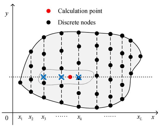
Figure 1.
Problem domain and node distribution for the DS-IMLS method.
Based on the idea of the DSM, the unknown is first regarded as a one-dimensional function of . Then, imposing the improved IMLS method with nonsingular weight functions on the node distribution , the approximation function on can be obtained as
where is the shape function determined by the improved IMLS method in one-dimensional space from Equation (4), and suppose is one of the nodes whose influence domain covers .
Next, the function is treated as the function on , and is approximated by the improved IMLS method on the split plane . Suppose the plane is discretized as , where is the number of the nodes on . Then we have
where is a node whose influence domain contains , and is the number, and is the shape function deduced from the splitting plane .
Coupling Equations (16) and (17), the approximation function of can be
Let . Suppose that the global number of in all discrete nodes of the problem domain is , . Then Equation (18) can be rewritten as
where is the shape function of the DS-IMLS method, and
The derivatives of the approximation function can be easily obtained as
where the subscript is defined as
The radii of the influence domain of nodes for the approximation of Equations (16) and (17) are, respectively, defined as
where and represent the distances between adjacent nodes in the direction and on the split plane, respectively. The and are the influence domain parameter determining the radii. To ensure the existence of the shape function, the radius of the influence domain should be large enough. We can adopt the adaptive algorithm to determine the radius so there is an appropriate number in the influence domain in the program.
Thus, the DS-IMLS method is proposed. In the DS-IMLS method, the weight function is not singular, and the approximation satisfies the Kronecker delta property. Since the DSM is used to divide the problem into a series of lower-dimensional problems, the complexity of the matrix calculation for calculating the approximation function and its derivative is reduced.
4. The Improved IEFG Method Based on the DS-IMLS Method
Consider the following two-dimensional potential problems
with the essential boundary condition
where is the boundary of , and are given functions.
The Galerkin weak form of Equation (27) is
where denotes the variation of function .
From the partial integral, it follows that
where
From the DS-IMLS method, the function can be approximated as
Substituting Equation (32) into Equation (30) yields
where
According to the arbitrariness of , the discretized equation of Equation (27) is
where
The shape functions of the DS-IMLS method have the interpolating property. Then the numerical solutions for two-dimensional potential problems can be obtained by directly substituting the essential boundary condition into Equation (35). Thus, the improved IEFG method based on the DS-IMLS method is presented for the potential problems.
5. Numerical Example
This section presents some examples to illustrate the effectiveness of the DS-IMLS method and the improved IEFG method. Three examples are given for studying the convergence and errors of the approximation function of the DS-IMLS method by using the known functions. In addition, two potential problems are solved by the improved IEFG method based on the DS-IMLS method. All numerical results are compared with those of the MLS or EFG methods. Both the MLS and DS-IMLS methods use second-order complete polynomial basis functions and cubic spline weight functions. In the MLS method, the node rectangular influence field of the following form is adopted:
where is a two-dimensional column vector representing the average distance between nodes in the and directions. To study the error, the average and maximum errors of the following form are defined:
where and are, respectively, the exact and numerical solutions at the node , and is the number of the discrete points used to calculate the errors.
The procedure for obtaining the approximation of the DS–IMS method and the solution of the improved IEFG method is as follows:
- (1)
- Input the parameters of the governing equation and geometric parameters.
- (2)
- Split the problem domain into L layers in the dimension splitting direction and determine the radius of influence domain for point . Suppose the set of splitting points is .
- (3)
- Discretize the plane by , .
- (4)
- For any given (x, y), get all nodes whose influence field covers x, and denote the subscript set as . Then calculate the corresponding shape functions by the improved IMLS method from and .
- (5)
- For every , find all nodes in whose influence domain covers . Suppose the global number is . Then calculate the by introducing the improved IMLS method into and .
- (6)
- Coupling Steps (4) and (5), the approximation function of can be obtained as . Thus, the approximation of the DS-IMLS method is presented.
- (7)
- Substitute the approximation and its derivatives into Equation (30), and then obtain the discrete equation of the potential problems.
- (8)
- Substitute the essential boundary condition into Equation (35) and solve Equation (35), and then obtain the node value . Thus, the solution of the improved IEFG method for two-dimensional potential problems is obtained.
5.1. The Examples of the DS-IMLS Method
Example 1.
Let, .
The approximation function is constructed from the known function by the DS-IMLS method or MLS approximation. When , and regular nodes distribution is used, the numerical approximations of the functions on the line are shown in Figure 2, and the approximations of are given in Figure 3. The corresponding approximated values of the second derivatives obtained by the MLS method are shown in Figure 4. It can be seen from these figures that the approximation function and its first and second derivatives of the DS-IMLS method are very consistent with the exact solutions and have higher accuracy than the MLS method.

Figure 2.
The numerical approximations of the functions obtained by the DS-IMLS method.
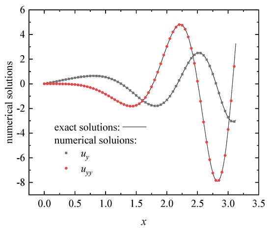
Figure 3.
The numerical approximations of the functions obtained by the DS-IMLS method.
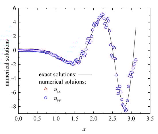
Figure 4.
The numerical approximations of obtained by the MLS method.
In order to analyze the influence of influence domain parameters on the error, regular points are used to calculate the average and maximum errors. The approximation functions of the DS-IMLS and MLS methods are constructed based on the regular nodes distribution. When , the average and maximum errors of the nodes for different influence domain parameters are shown in Figure 5a. When fixing , the corresponding errors are shown in Figure 5b. The errors of the MLS method for different influence domain parameter values are depicted in Figure 6. For the quadratic basis function, the DS-IMLS method has higher stability on the influence domain parameters and has high calculation accuracy when the value is greater than 3.
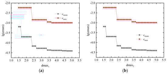
Figure 5.
The average and maximum errors obtained by the DS-IMLS method for (a) different values of with fixed ; (b) different values of with fixed .
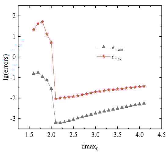
Figure 6.
The average and maximum errors obtained by the MLS method for different influence domain parameters .
To analyze the convergence of the approximation function with respect to node spacing, when 5 × 5, 9 × 9, 13 × 13, 17 × 17, and 21 × 21 regular node distributions are respectively adopted, the average discrete point errors of the DS-IMLS and MLS methods at 3030 points are shown in Figure 7. The corresponding maximum point errors are given in Figure 8. Here, , and . It can be seen that the approximation function of the DS-IMLS method gradually converges to the exact solution with the increase of the number of nodes and has a higher convergence order than the MLS method. Let represent the uniformly distributed random numbers on (0,1) generated by Matlab and be the node spacing. When the perturbation of is added on the nodes and , the errors of and under the irregular node distribution are plotted in Figure 9. This figure shows that the approximation of the DS-IMLS method also has high accuracy under irregular nodes distribution.
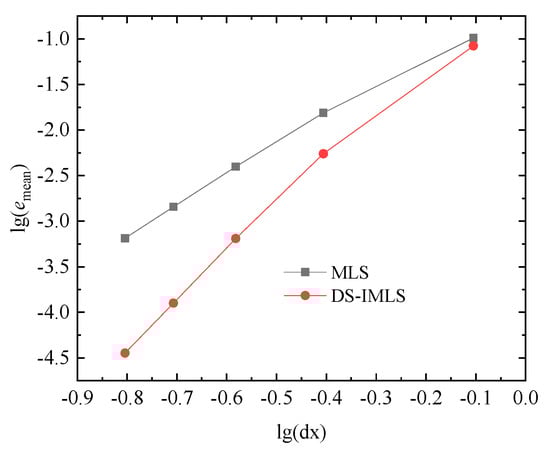
Figure 7.
The average discrete point errors of the DS-IMLS and MLS methods for the different node distances of 55, 99, 1313, 1717, 2121 regular node distributions.
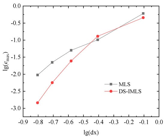
Figure 8.
The maximum errors of the DS-IMLS and MLS methods for the different node distances of 55, 99, 1313, 1717, 2121 regular node distributions.
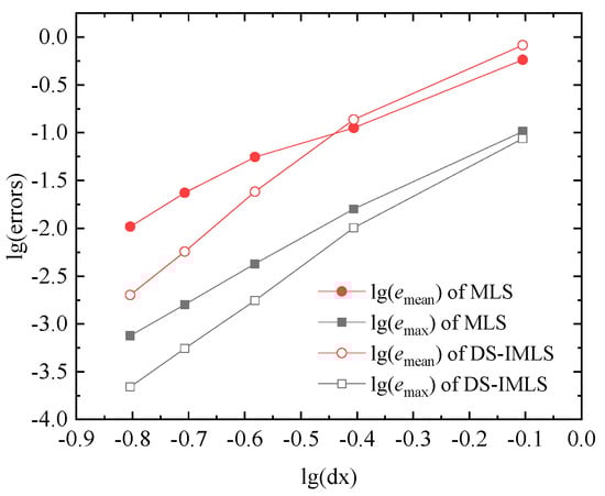
Figure 9.
The errors and of the MLS and DS-IMLS methods under the irregular node distribution obtained by small random disturbance.
Example 2.
Let, .
In this example, regular nodes distribution is used to construct the approximation function. The numerical approximations of the on the line are plotted in Figure 10 by using the DS-IMLS method with . The corresponding numerical results of the second derivatives obtained by the DS-IMLS and MLS methods are shown in Figure 11. We can see that the approximation function and its derivatives of the DS-IMLS method fit the exact solution very well.
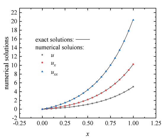
Figure 10.
The numerical approximations of the functions on line obtained by the DS-IMLS method for Example 2.
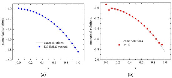
Figure 11.
The numerical approximations of on line obtained by the DS-IMLS (a) and MLS (b) methods for Example 2.
When fixing , the average and maximum point errors of the regular calculation point are shown in Figure 12a for different values of . Fixing , the corresponding errors for different values of are listed in Figure 12b. The effect of the influence domain parameter on the MLS method is shown in Figure 13. It can still be seen that when the value of the influence domain parameter reaches 3, the DS-IMLS method has better calculation accuracy.
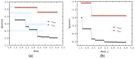
Figure 12.
The errors on the regular calculation point obtained by the DS-IMLS method for (a) different with ; (b) different with .
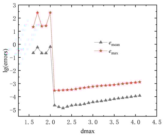
Figure 13.
The errors obtained by the MLS method for different influence domain parameters .
When , and , the errors and for the different node distance of 55, 99, 1313, 1717, 2121 regular node distributions are respectively shown in Figure 14 and Figure 15 by the DS-IMLS and MLS methods. The DS-IMLS method has a higher order of convergence than the MLS method.
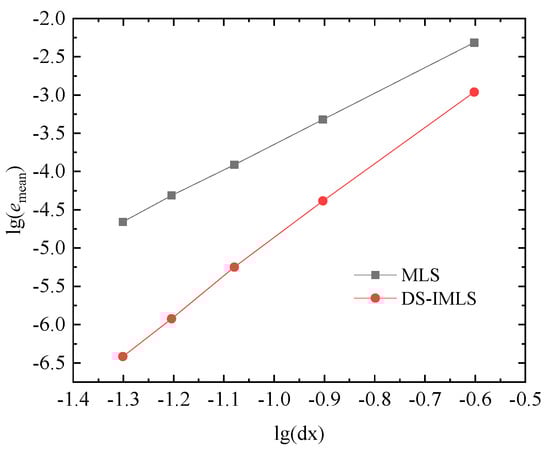
Figure 14.
The errors of the DS-IMLS and MLS methods for different node distances of 55, 99, 1313, 1717, 2121 regular node distributions.
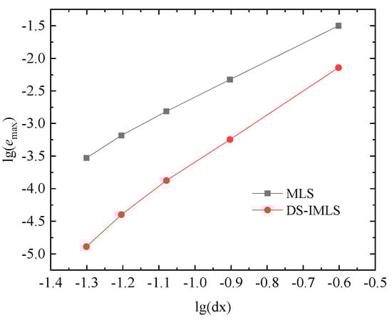
Figure 15.
The maximum errors of the DS-IMLS and MLS methods for the different node distance for Example 2.
Example 3.
Let, .
When regular nodes distribution is used and , the approximation and its first and second derivatives on the line are plotted in Figure 16. The partial derivatives of the approximation function concerning are shown in Figure 17. The approximation of the DS-IMLS method is also consistent with the exact function. Let . When using the 55, 99, 1313, 1717, and 2121 regular node distributions, the errors and obtained by the DS-IMLS and MLS methods are shown in Figure 18 and Figure 19, respectively. These two figures show that the approximation functions of the DS-IMLS and MLS methods are convergent to the exact solutions, and the DS-IMLS method has a higher convergence rate.
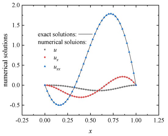
Figure 16.
The approximations of the functions on the line obtained by the DS-IMLS method for Example 3.
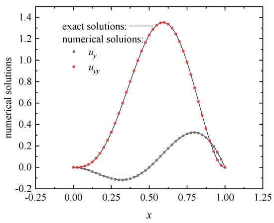
Figure 17.
The approximations of the functions on the line obtained by the DS-IMLS method for Example 3.
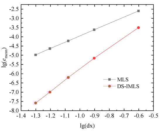
Figure 18.
The errors obtained by the DS-IMLS and MLS methods for the different node distances of 55, 99, 1313, 1717, 2121 regular node distributions of Example 3.
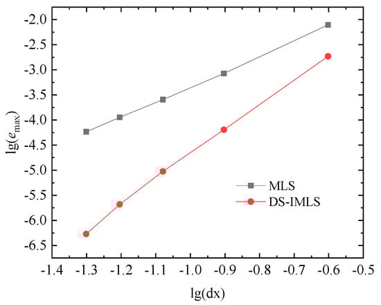
Figure 19.
The maximum errors obtained by the DS-IMLS and MLS methods for the different node distances of Example 3.
5.2. The Examples for the Improved IEFG Method Based on the DS-IMLS Method
Example 4.
Considering a temperature field governed by Laplace’s equation
The essential boundary conditions are used and deduced from the analytical temperature solution of
When regular nodes distribution is used and , , the improved IEFG method of this paper and EFG methods are used to solve this potential problem. In the EFG method, the Lagrange multiplier method is applied to enforce the essential boundary condition. The exact and numerical solutions obtained with the improved IEFG and EFG methods on the line are listed in Figure 20. The corresponding absolute errors of numerical solutions of the improved IEFG and EFG methods are plotted in Figure 21. It is clear that the solutions of the improved IEFG and EFG methods are very consistent with the analytical solutions, but the improved IEFG method based on the DS-IMLS method has a smaller calculation error than the EFG method.
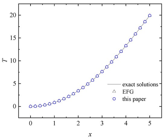
Figure 20.
The exact and numerical solutions on the line obtained by the improved IEFG and EFG methods.
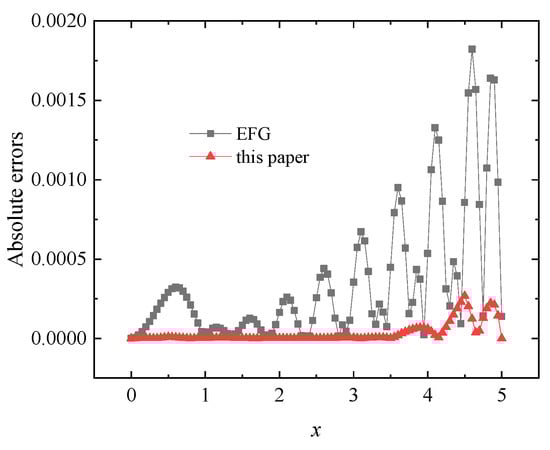
Figure 21.
The absolute errors of numerical solutions on the line obtained by the improved IEFG and EFG methods.
Example 5.
Considering a potential problem governed by
with
The essential boundary conditions are used, and the analytical solution is
Let , . Using the regular nodes distribution, the numerical solutions on the line solved by the improved IEFG and EFG methods are shown in Figure 22. The corresponding absolute errors are shown in Figure 23. For the two-dimensional potential problem, this example again illustrates that the improved IEFG method based on the DS-IMLS method has a smaller calculation error than the EFG method.
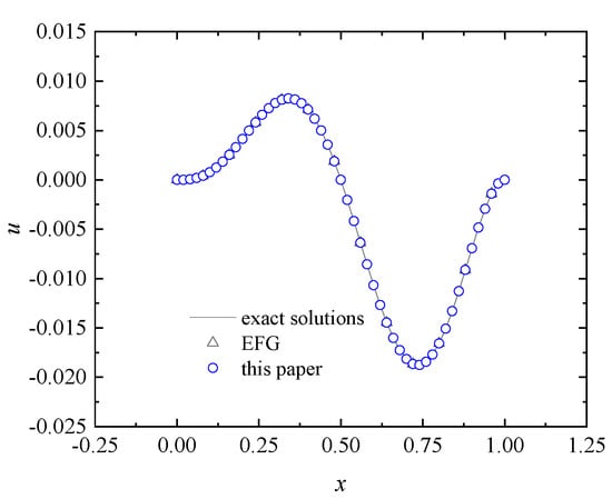
Figure 22.
The exact and numerical solutions on the line obtained by the EFG and improved IEFG methods of this paper for Example 5.
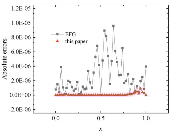
Figure 23.
The absolute errors of solutions on the line obtained by the EFG and improved IEFG methods of this paper for Example 5.
Example 6.
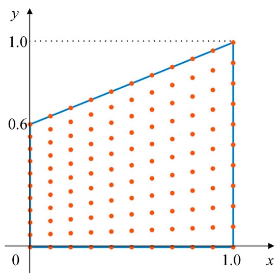
The example considered is a potential problem with a trapezoidal field as shown in Figure 24. The source term is
Figure 24.
A trapezoidal field for Example 6.
The analytical solution is
Let , . When the regular nodes (shown in Figure 24) and the essential boundary condition are used, the numerical and exact solutions on the line are shown in Figure 25. We can see that the numerical solution of this paper is in good agreement with the exact solution. When using different node distributions shown in Table 1, the corresponding average errors of the node distribution are given in Table 1. When 1181 regular nodes are used, the EFG method cannot obtain the numerical solutions. It can be seen from the table that both the EFG and improved IEFG methods have high calculation accuracy. When the difference of the node spacings in the x and y directions is very large, the improved IEFG method can still obtain high accuracy, but the EFG method may not obtain a numerical solution. Moreover, reducing the spacing dx of dimension splitting is more conducive for the improved IEFG method of this paper to improve the accuracy than reducing the node spacing on the split plane. When 1111, 2111,, nodes are adopted, the relationships between the average error and CPU time for the EFG and the method of this paper are shown in Figure 26. It can be seen from the figure that when the node spacing in X and Y directions is quite different, the IEFG method based on the DS-IMLS method has high calculation efficiency.
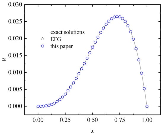
Figure 25.
The exact and numerical solutions on the line obtained by the EFG and improved IEFG methods of this paper for Example 6.

Table 1.
The average errors of the EFG and improved IEFG methods for different nodes.
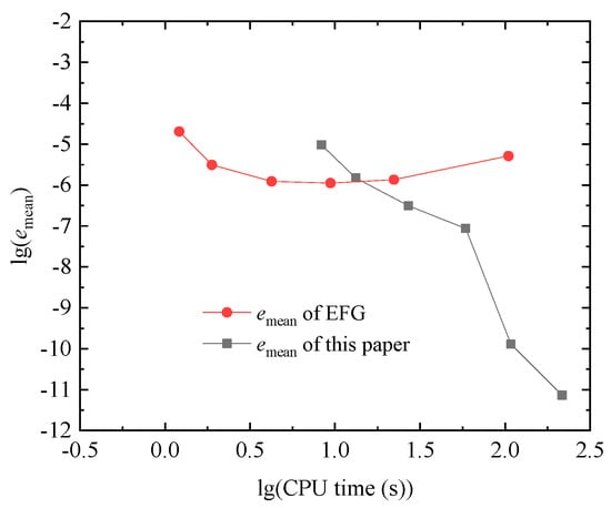
Figure 26.
The relationships between the average error and CPU time for the EFG and the method of this paper under the 11 × 11, 21 × 11,, 81 × 11 nodes.
6. Conclusions
By introducing the DSM into the improved IMLS method with a nonsingular weight function, this paper presents a new hybrid method to obtain the shape function of the meshless method, which is called the dimension splitting–interpolating moving least squares (DS-IMLS) method. Then based on the Galerkin weak form and the DS-IMLS method, the improved IEFG method for the two-dimensional potential problems is also presented. The weight function used in the DS-IMLS method is nonsingular, and the approximation function has the characteristics of the Kronecker delta function. Then the improved IEFG method based on the DS-IMLS method can directly impose essential boundary conditions. Since the DSM can decompose the problem into a series of lower-dimensional problems, the DS-IMLS method can reduce the matrix dimension and complexity in calculating the shape function. The derivatives of the approximation function in the DS-IMLS method can be easily calculated. For a two-dimensional space, the shape function is calculated from a series of one-dimensional spaces, and then the order of the matrix that needs to be inverted will be greatly reduced. The DS-IMLS method has high calculation accuracy for anisotropic node distribution. When the difference between the node spacings in the x and y directions is very large, the DS-IMLS method still has a good calculation effect. Several examples demonstrated that the approximation function and its derivatives of the DS-IMLS and the improved IEFG methods have high accuracy in the regular problem domain.
Author Contributions
Conceptualization, J.W. and F.S.; methodology, J.W. and F.S.; software, J.W. and F.S.; writing—original draft preparation, J.W. and F.S.; writing—review and editing, J.W. and R.C. All authors have read and agreed to the published version of the manuscript.
Funding
This research was funded by the Natural Science Foundation of Zhejiang Province, China (Grant Nos. LY20A010021, LY20G030025, LY19A010002, LY18F020026), and the Ningbo Natural Science Foundation of China (Grant No. 202003N4142).
Institutional Review Board Statement
Not applicable.
Informed Consent Statement
Not applicable.
Data Availability Statement
Not applicable.
Conflicts of Interest
The authors declare no conflict of interest.
References
- Gu, Y.; Fan, C.; Xu, R. Localized method of fundamental solutions for large-scale modeling of two-dimensional elasticity problems. Appl. Math. Lett. 2019, 93, 8–14. [Google Scholar] [CrossRef]
- Zhang, T.; Li, X. Variational multiscale interpolating element-free Galerkin method for the nonlinear darcy–forchheimer model. Comput. Math. Appl. 2020, 79, 363–377. [Google Scholar] [CrossRef]
- Gu, Y.; Fan, C.; Qu, W.; Wang, F. Localized method of fundamental solutions for large-scale modelling of three-dimensional anisotropic heat conduction problems–theory and Matlab code. Comput. Struct. 2019, 220, 144–155. [Google Scholar] [CrossRef]
- Wang, J.; Sun, F. A hybrid variational multiscale element-free Galerkin method for convection-diffusion problems. Int. J. Appl. Mech. 2019, 11, 1950063. [Google Scholar] [CrossRef]
- Lin, J.; Xu, Y.; Zhang, Y. Simulation of linear and nonlinear advection–diffusion–reaction problems by a novel localized scheme. Appl. Math. Lett. 2020, 99, 106005. [Google Scholar] [CrossRef]
- Gu, Y.; Sun, H. A meshless method for solving three-dimensional time fractional diffusion equation with variable-order derivatives. Appl. Math. Model. 2020, 78, 539–549. [Google Scholar] [CrossRef]
- Abbaszadeh, M.; Khodadadian, A.; Parvizi, M.; Dehghan, M.; Heitzinger, C. A direct meshless local collocation method for solving stochastic Cahn–Hilliard–cook and stochastic swift–Hohenberger equations. Eng. Anal. Bound. Elem. 2019, 98, 253–264. [Google Scholar] [CrossRef]
- Selim, B.A.; Liu, Z. Impact analysis of functionally-graded graphene nanoplatelets-reinforced composite plates laying on Winkler-Pasternak elastic foundations applying a meshless approach. Eng. Struct. 2021, 241, 112453. [Google Scholar] [CrossRef]
- Almasi, F.; Shadloo, M.S.; Hadjadj, A.; Ozbulut, M.; Tofighi, N.; Yildiz, M. Numerical simulations of multi-phase electro-hydrodynamics flows using a simple incompressible smoothed particle hydrodynamics method. Comput. Math. Appl. 2021, 81, 772–785. [Google Scholar] [CrossRef]
- Lancaster, P.; Salkauskas, K. Surfaces generated by moving least squares methods. Math. Comput. 1981, 37, 141–158. [Google Scholar] [CrossRef]
- Li, Y.; Liu, G.R. An element-free smoothed radial point interpolation method (EFS-RPIM) for 2d and 3d solid mechanics problems. Comput. Math. Appl. 2019, 77, 441–465. [Google Scholar] [CrossRef]
- Li, J.; Feng, X.; He, Y. Rbf-based meshless local Petrov Galerkin method for the multi-dimensional convection–diffusion-reaction equation. Eng. Anal. Bound. Elem. 2019, 98, 46–53. [Google Scholar] [CrossRef]
- Lin, J.; Yu, H.; Reutskiy, S.; Wang, Y. A meshless radial basis function based method for modeling dual-phase-lag heat transfer in irregular domains. Comput. Math. Appl. 2021, 85, 1–17. [Google Scholar] [CrossRef]
- Cavoretto, R.; De Rossi, A. Adaptive meshless refinement schemes for RBF-PUM collocation. Appl. Math. Lett. 2019, 90, 131–138. [Google Scholar] [CrossRef] [Green Version]
- Khan, M.N.; Hussain, I.; Ahmad, I.; Ahmad, H. A local meshless method for the numerical solution of space-dependent inverse heat problems. Math. Methods Appl. Sci. 2021, 44, 3066–3079. [Google Scholar] [CrossRef]
- Fu, Z.; Chu, W.; Yang, M.; Li, P.; Fan, C. Estimation of tumor characteristics in a skin tissue by a meshless collocation solver. Int. J. Comput. Methods 2021, 18, 2041009. [Google Scholar] [CrossRef]
- Wang, L.; Qian, Z. A meshfree stabilized collocation method (SCM) based on reproducing kernel approximation. Comput. Methods Appl. Mech. Eng. 2020, 371, 113303. [Google Scholar] [CrossRef]
- Beel, A.; Kim, T.; Jiang, W.; Song, J. Strong form-based meshfree collocation method for wind-driven ocean circulation. Comput. Methods Appl. Mech. Eng. 2019, 351, 404–421. [Google Scholar] [CrossRef]
- Almasi, A.; Beel, A.; Kim, T.; Michopoulos, J.G.; Song, J. Strong-form collocation method for solidification and mechanical analysis of polycrystalline materials. J. Eng. Mech. 2019, 145, 04019082. [Google Scholar] [CrossRef]
- Almasi, A.; Kim, T.; Laursen, T.A.; Song, J. A strong form meshfree collocation method for frictional contact on a rigid obstacle. Comput. Methods Appl. Mech. Eng. 2019, 357, 112597. [Google Scholar] [CrossRef]
- Park, S.I.; Lee, S.; Almasi, A.; Song, J. Extended IFC-based strong form meshfree collocation analysis of a bridge structure. Autom. Constr. 2020, 119, 103364. [Google Scholar] [CrossRef]
- Li, X.; Dong, H. An element-free Galerkin method for the obstacle problem. Appl. Math. Lett. 2021, 112, 106724. [Google Scholar] [CrossRef]
- Abbaszadeh, M.; Dehghan, M. The reproducing kernel particle Petrov–Galerkin method for solving two-dimensional nonstationary incompressible boussinesq equations. Eng. Anal. Bound. Elem. 2019, 106, 300–308. [Google Scholar] [CrossRef]
- Liu, Z.; Wei, G.; Wang, Z. Numerical analysis of functionally graded materials using reproducing kernel particle method. Int. J. Appl. Mech. 2019, 11, 1950060. [Google Scholar] [CrossRef]
- Abbaszadeh, M.; Dehghan, M. Direct meshless local Petrov–Galerkin (DMLPG) method for time-fractional fourth-order reaction–diffusion problem on complex domains. Comput. Math. Appl. 2020, 79, 876–888. [Google Scholar] [CrossRef]
- Zhu, T.; Zhang, J.; Atluri, S.N. A local boundary integral equation (LBIE) method in Comput. Mech., and a meshless discretization approach. Comput. Mech. 1998, 21, 223–235. [Google Scholar] [CrossRef]
- Cheng, J. Residential land leasing and price under public land ownership. J. Urban Plan. Dev. 2021, 147, 05021009. [Google Scholar] [CrossRef]
- Cheng, J. Analysis of commercial land leasing of the district governments of Beijing in China. Land Use Policy 2021, 100, 104881. [Google Scholar] [CrossRef]
- Cheng, J. Analyzing the factors influencing the choice of the government on leasing different types of land uses: Evidence from Shanghai of China. Land Use Policy 2020, 90, 104303. [Google Scholar] [CrossRef]
- Cheng, J. Data analysis of the factors influencing the industrial land leasing in shanghai based on mathematical models. Math. Probl. Eng. 2020, 2020. [Google Scholar] [CrossRef] [Green Version]
- Belytschko, T.; Lu, Y.Y.; Gu, L. Element-free Galerkin methods. Int. J. Numer. Methods Eng. 1994, 37, 229–256. [Google Scholar] [CrossRef]
- Singh, R.; Singh, K.M. Interpolating meshless local Petrov-Galerkin method for steady state heat conduction problem. Eng. Anal. Bound. Elem. 2019, 101, 56–66. [Google Scholar] [CrossRef]
- Wang, F.; Gu, Y.; Qu, W.; Zhang, C. Localized boundary knot method and its application to large-scale acoustic problems. Comput. Methods Appl. Mech. Eng. 2020, 361, 112729. [Google Scholar] [CrossRef]
- Liew, K.M.; Cheng, Y.; Kitipornchai, S. Boundary element-free method (BEFM) and its application to two-dimensional elasticity problems. Int. J. Numer. Methods Eng. 2006, 65, 1310–1332. [Google Scholar] [CrossRef]
- Zheng, G.; Cheng, Y. The improved element-free Galerkin method for diffusional drug release problems. Int. J. Appl. Mech. 2020, 12, 2050096. [Google Scholar] [CrossRef]
- Peng, M.; Cheng, Y. A boundary element-free method (BEFM) for two-dimensional potential problems. Eng. Anal. Bound. Elem. 2009, 33, 77–82. [Google Scholar] [CrossRef]
- Zhang, L.W.; Liew, K. An improved moving least-squares ritz method for two-dimensional elasticity problems. Appl. Math. Comput. 2014, 246, 268–282. [Google Scholar] [CrossRef]
- Liew, K.M.; Feng, C.; Cheng, Y.; Kitipornchai, S. Complex variable moving least-squares method: A meshless approximation technique. Int. J. Numer. Methods Eng. 2007, 70, 46–70. [Google Scholar] [CrossRef]
- Chen, L.; Li, X. A complex variable boundary element-free method for the Helmholtz equation using regularized combined field integral equations. Appl. Math. Lett. 2020, 101, 106067. [Google Scholar] [CrossRef]
- Cheng, H.; Peng, M.; Cheng, Y.; Meng, Z. The hybrid complex variable element-free Galerkin method for 3d elasticity problems. Eng. Struct. 2020, 219, 110835. [Google Scholar] [CrossRef]
- Liu, D.; Cheng, Y.M. The interpolating element-free Galerkin (IEFG) method for three-dimensional potential problems. Eng. Anal. Bound. Elem. 2019, 108, 115–123. [Google Scholar] [CrossRef]
- Chen, S.S.; Xu, C.J.; Tong, G.S. A meshless local natural neighbour interpolation method to modeling of functionally graded viscoelastic materials. Eng. Anal. Bound. Elem. 2015, 52, 92–98. [Google Scholar] [CrossRef]
- Chen, S.; Wang, W.; Zhao, X. An interpolating element-free Galerkin scaled boundary method applied to structural dynamic analysis. Appl. Math. Model. 2019, 75, 494–505. [Google Scholar] [CrossRef]
- Wang, Q.; Zhou, W.; Feng, Y.T.; Ma, G.; Cheng, Y.; Chang, X. An adaptive orthogonal improved interpolating moving least-square method and a new boundary element-free method. Appl. Math. Comput. 2019, 353, 347–370. [Google Scholar] [CrossRef]
- Wang, J.; Sun, F.; Xu, Y. Research on error estimations of the interpolating boundary element free-method for two-dimensional potential problems. Math. Probl. Eng. 2020, 2020, 6378745. [Google Scholar] [CrossRef]
- Sun, F.X.; Wang, J.F.; Cheng, Y.M.; Huang, A.X. Error estimates for the interpolating moving least-squares method in n-dimensional space. Appl. Numer. Math. 2015, 98, 79–105. [Google Scholar] [CrossRef]
- Wang, J.F.; Sun, F.; Cheng, Y.; Huang, A.X. Error estimates for the interpolating moving least-squares method. Appl. Math. Comput. 2014, 245, 321–342. [Google Scholar] [CrossRef]
- Abbaszadeh, M.; Dehghan, M. Numerical and analytical investigations for neutral delay fractional damped diffusion-wave equation based on the stabilized interpolating element free Galerkin (IEFG) method. Appl. Numer. Math. 2019, 145, 488–506. [Google Scholar] [CrossRef]
- Wu, Q.; Liu, F.B.; Cheng, Y.M. The interpolating element-free Galerkin method for three-dimensional elastoplasticity problems. Eng. Anal. Bound. Elem. 2020, 115, 156–167. [Google Scholar] [CrossRef]
- Abbaszadeh, M.; Dehghan, M. Investigation of heat transport equation at the microscale via interpolating element-free Galerkin method. Eng. Comput. 2021, 1–17. [Google Scholar]
- Wang, J.; Sun, F. An interpolating meshless method for the numerical simulation of the time-fractional diffusion equations with error estimates. Eng. Comput. 2019, 37, 730–752. [Google Scholar] [CrossRef]
- Wang, J.; Wang, J.; Sun, F.; Cheng, Y. An interpolating boundary element-free method with nonsingular weight function for two-dimensional potential problems. Int. J. Comput. Methods 2013, 10, 1350043. [Google Scholar] [CrossRef]
- Sun, F.; Wang, J.; Cheng, Y. An improved interpolating element-free Galerkin method for elastoplasticity via nonsingular weight functions. Int. J. Appl. Mech. 2016, 8, 1650096. [Google Scholar] [CrossRef]
- Wu, S.; Xiang, Y. A coupled interpolating meshfree method for computing sound radiation in infinite domain. Int. J. Numer. Methods Eng. 2018, 113, 1466–1487. [Google Scholar] [CrossRef]
- Li, X. An interpolating boundary element-free method for three-dimensional potential problems. Appl. Math. Model. 2015, 39, 3116–3134. [Google Scholar] [CrossRef]
- Liu, F.; Wu, Q.; Cheng, Y. A meshless method based on the nonsingular weight functions for elastoplastic large deformation problems. Int. J. Appl. Mech. 2019, 11, 1950006. [Google Scholar] [CrossRef]
- Chen, H.; Li, K.; Wang, S. A dimension split method for the incompressible Navier–Stokes equations in three dimensions. Int. J. Numer. Methods Fluids 2013, 73, 409–435. [Google Scholar] [CrossRef]
- Wang, J.; Sun, F. A hybrid generalized interpolated element-free Galerkin method for stokes problems. Eng. Anal. Bound. Elem. 2020, 111, 88–100. [Google Scholar] [CrossRef]
- Meng, Z.; Cheng, H.; Ma, L.; Cheng, Y. The dimension splitting element-free Galerkin method for 3d transient heat conduction problems. Sci. China Phys. Mech. Astron. 2019, 62, 1–12. [Google Scholar] [CrossRef]
- Wu, Q.; Peng, M.J.; Fu, Y.D.; Cheng, Y.M. The dimension splitting interpolating element-free Galerkin method for solving three-dimensional transient heat conduction problems. Eng. Anal. Bound. Elem. 2021, 128, 326–341. [Google Scholar] [CrossRef]
- Wu, Q.; Peng, M.; Cheng, Y. The interpolating dimension splitting element-free Galerkin method for 3d potential problems. Eng. Comput. 2021, 1–15. [Google Scholar] [CrossRef]
Publisher’s Note: MDPI stays neutral with regard to jurisdictional claims in published maps and institutional affiliations. |
© 2021 by the authors. Licensee MDPI, Basel, Switzerland. This article is an open access article distributed under the terms and conditions of the Creative Commons Attribution (CC BY) license (https://creativecommons.org/licenses/by/4.0/).