A Square-Root Factor-Based Multi-Population Extension of the Mortality Laws

Abstract

In this paper, we present and calibrate a multi-population stochastic mortality model based on latent square-root affine factors of the Cox-Ingersoll and Ross type. The model considers a generalization of the traditional actuarial mortality laws to a stochastic, multi-population and time-varying setting. We calibrate the model to fit the mortality dynamics of UK males and females over the last 50 years. We estimate the optimal states and model parameters using quasi-maximum likelihood techniques.

1. Introduction

Mortality laws are considered traditional actuarial models that describe the link between death probabilities (or the force of mortality) and the age of the individuals. However, it is very soon after continuous-time stochastic mortality models started developing that [1] proposed the use of latent factors to generalize mortality laws to a stochastic continuous-time setting. In the proposed framework, a set of time-varying stochastic components and parameters affected the evolution of mortality rates at different ages. In particular, [1] calibrated the one-year death probabilities of several ages of the Dutch population to 2- or 3-factor Gaussian models that extended the first and second Makeham’s and Thiele’s laws to a stochastic setting. The authors of [2] built on a similar setup to propose a general multi-population stochastic extension of mortality laws. There, the mortality intensities of several populations were affine functions of affine latent factors. Different populations and sub-populations within them had different mortality dynamics because they depended on some common factors—shared among population groups—and certain idiosyncratic factors, which were population-specific. Population-specific parameters interact with such factors to reproduce the age–mortality relation. While the setting described in [2] was very general, the implementation was restricted to the use of Gaussian factors. The Gaussian factors have the advantage of being easier to calibrate. However, Gaussian factors have the disadvantage of allowing for negative mortality intensities with non-negative probabilities. That is a relevant shortcoming, for instance, for annuity pricing purposes. In their work, [2] described the application of a 4-population 3-factor law, they estimated through the use of a sequential Kalman filter. In this paper, we advance the previous work and focus on the case in which factors are non-Gaussian, which has not been previously undertaken in the actuarial literature. While several other works have used factor models to represent the evolution of mortality intensity of multiple ages simultaneously in continuous time (see [3,4], for instance), only a few, however, have considered non-Gaussian factors [5]. In contrast to that paper, which calibrated a model for a restricted portion of the mortality curve of the two-population case, our work tries to parsimoniously capture the evolution of mortality of the entire curve or a large fraction of the ages. Further, this work implements a two-population model that lies within the general framework described in [2] and considers factors modeled as square-root processes à la [6]. Finally, we estimate a stochastic multi-population version of the second Makeham’s law and a modification of Thiele’s law to fit the observed mortality death rates of United Kingdom females and males from 1967 to 2017 by exploiting the state-space representation of our model. To achieve that, we take a centralized data fusion approach, assuming all observations come from the same source while at the same time assuming Gaussian measurement errors. In addition, the non-normality of the state process dynamics, which violates the assumptions under which the standard Kalman filter produces optimal state estimates and an exact log-likelihood for the model, was accounted for. Specifically, we followed [7] and modified the Kalman filter structure to introduce non-linearity and apply thus a Quasi-Maximum Likelihood approach. While producing a possibly conditionally biased estimate, the Kalman filter we implemented remains the optimal linear filter [8].

The paper is structured as follows. Section 2 draws a historical picture of mortality laws and provides some motivation for our work. Section 3 describes the modeling setup. Section 4 specifies the state-space form of our model. Finally, Section 5 presents our application of the stochastic multi-population version of the Second Makeham’s and a 3-factor modified version of Thiele’s mortality law to the UK male and female population.

2. Mortality Laws: Motivation

At an aggregate level, the most important covariate in explaining individual mortality is age. Indeed, mortality rates have an obvious relation with age. Historically, mortality rates have been high for infants due to the perils of labor and their fragility, increasing at older ages due to biological aging. Due to this persistent phenomenon, actuaries started describing the relation between mortality rates and age through mathematical models, starting from the XVIII century. These mathematical models are of the form:

$${\mu }_x=f(x;\xi ),$$

where ${\mu }_x$ denotes the mortality intensity of an age x and $\xi$ is a set of parameters. The most famous laws were introduced in the XIX century. In what follows, we give an account of these models. The Gompertz law describes the mortality intensity ${\mu }_x$ at age x as a function of two parameters:

$${\mu }_x=B{c}^x.$$

It captures the phenomenon of so-called senescent mortality, since it assumes an exponential increment in the mortality intensity with age. Makeham laws, proposed in 1867 and 1890 respectively, have the following forms:

$${\mu }_x=A+B{c}^x;$$

$${\mu }_x=A+Hx+B{c}^x,$$

where, together with the exponential term as in the Gompertz law, a baseline mortality level (A) and a linear term ($Hx$) are added. The Thiele law, dating back to 1871, aimed at capturing the whole mortality–age curve, by considering, together with the exponential term à la Gompertz, a term that tries to capture the spike of the curve at age 0 associated with infant mortality and a term to reproduce the so-called accident hump:

$${\mu }_x=A{e}^{-Bx}+C{e}^{-D{(x-E)}^2}+F{G}^x.$$

In the last century, several other laws have been proposed. They combine additional terms and different functional forms. Other prominent examples are Heligman–Pollard’s laws and the Perks laws, which identify a functional relation between the death rate q or the odds ratio $\frac{q}{p}$ (i.e., the ratio between the death rate and the survival probability p), and age. The interested reader may refer to the book [9] for a more detailed account.

The success of traditional mortality laws is due to their ability to capture parsimoniously in a deterministic fashion the relation between the mortality intensity and age. The functional forms used are able to capture the most important trends in such relation, such as the infant mortality pattern and the old-age increase in mortality rates. However, the age-patterns profiles have been changing in time. Thus, the fit of the mortality laws to the observed data of a certain population over different calendar years would produce different parameter estimates. To capture this issue and be able to describe mortality dynamics in a model, while maintaining the traditional actuarial approach of mortality laws, Schrager [1] suggested modeling some parameters in the mortality laws as stochastic factors. Indeed, the introduction of stochastic factors can capture the time trends in human mortality development and the uncertainty surrounding them. The authors of [2] extended that setup to describe the mortality intensity of multiple populations. In that framework, which will be reviewed more properly in the next section, the mortality intensity of individuals of different populations, at different ages and calendar years, is modeled as a function of population-specific parameters and factors. Such an extension allows to jointly describe the mortality intensity of several general populations or sub-groups (socio-economic groups), their evolution in time, and their uncertainty through traditional mortality laws.

3. The Model

In this section, we present a square-root factor-based approach to stochastic mortality modeling, building on the work in [2]. The mortality intensity of different ages of several populations is modeled parsimoniously as a function of some population-specific parameters and a set of latent factors described by a multivariate Cox, Ingersoll, and Ross (1985) process.

3.1. Mortality Intensity and Information

Our continuous-time modeling framework follows the approach first proposed by [10], in which the death process of an individual is described as the first jump time of a Poisson process with stochastic intensity. Mortality intensity is indeed such intensity. This modeling approach parallels the paradigm extensively used in credit risk modeling, in which firm default is similarly represented [11].

Let us introduce a probability space $(\mathrm{\Omega },\mathcal{F},{\left({\mathcal{F}}_t\right)}_{t\ge 0},\mathbb{P})$, with $\mathbb{P}$ denoting a (historical) probability measure. The filtration $\left\{{\mathcal{F}}_t:0\le t\le T\right\}$ satisfies the usual properties of right-continuity and completeness and contains the information on the mortality rates, coming from the historical life tables, contained in sub-filtration ${\mathcal{G}}_t$, as well as the knowledge on whether the individual is alive at time t, contained in the sub-filtration ${\mathcal{H}}_t$. Hence, ${\mathcal{F}}_t={\mathcal{G}}_t\cup {\mathcal{H}}_t$.

We assume there exist $J\in {\mathbb{N}}^{+}$ populations of interest, indexed by $j\in \mathit{J}=\{1,\dots ,J\}$. Our interest is in modeling the evolution of the mortality intensities of sets of ages (cohorts of individuals sharing the same year of birth) belonging to these different populations. We define the set of ages of interest in population j as ${\mathit{X}}^j:=\{x_{min}^j,\cdots ,x_{max}^j\}$, where integer ages are ordered from the smallest, $x_{min}$, to the biggest, $x_{max}$. In principle, we can consider different sets of ages for different populations. Let us define as ${\mu }_{x+t}^j\left(t\right)$ the set of predictable processes that represent the time t mortality intensity of an age $x+t$ belonging to the cohort aged x at time t.

The mortality intensity of individuals belonging to population j depends on a population-specific set of parameters, ${\gamma }^j$ and on a vector of unobservable stochastic factors ${\mathit{Y}}^j\left(t\right):={[Y_1^j\left(t\right),\dots ,Y_N^j\left(t\right)]}^T,j\in \mathit{J}$, $N\in {\mathbb{N}}^{++}$. The value of these factors represents the mortality trend level, which decreases and represents improvements to longevity due to progress in medicine, food availability, health habits, living conditions, and individual well-being.

We consider that all J populations are affected by the same innovations, described by a vector $\mathit{Z}\left(t\right)$ of Brownian noise. However, responses to such changes may differ across populations because factors can be population-specific and because these factors influence population mortality due to the population-specific parameters. Formally, the mortality intensity at time t of an age $x+t$, belonging to population j, ${\mu }_{x+t}^j\left(t\right)$, is described by a functional of the vector of state processes ${\mathit{Y}}^j$:

$$\begin{array}{c}\hfill {\mu }_{x+t}^j(t;x):=R^j({\mathit{Y}}^j\left(t\right),x,x+t,t,{\gamma }^j).\end{array}$$

(1)

Notice that the functional $R^j$ can in principle depend on the age $x+t$, the cohort x and calendar time t separately. We specify this functional further by assuming it has an affine dependence on the state-vector process. We define then two sets of population-specific functions $g_0^j(x+t,t,x)$ and

$${\mathit{g}}^j(x+t,t,x):={[g_1^j(x+t,t,x),\dots ,g_N^j(x+t,t,x)]}^{{}^{\prime }},$$

where $g_i^j:{\left({\mathbb{R}}^{+}\right)}^3\to {\mathbb{R}}^{+},i\in \{0,1,\dots ,N\}$ are age $x+t$, time t and cohort x–dependent functions for the j-th population, so that

$$\begin{array}{cc}\hfill & R^j({\mathit{Y}}^j\left(s\right);x+t,t,x):=g_0^j(x+t,t,x)+{\mathit{g}}^j(x+t,t,x)·{\mathit{Y}}^j\left(t\right),\hfill \end{array}$$

where · denotes the scalar product.

3.2. Stochastic Mortality Laws

We take advantage of the above setup to generalize the most common mortality laws we reviewed in Section 2:

• Gompertz’s law:

  $${\mu }_{x+t}^j\left(t\right):=Y_1^j\left(t\right){\left({\gamma }^j\right)}^{x+t}.$$
  In this case, ${\mathit{g}}^j(x+t,t,x):=\left[{\left({\gamma }^j\right)}^{x+t}\right]$, while ${\mathit{Y}}^j\in \mathbb{R}$.
• First Makeham law:

  $${\mu }_{x+t}^j\left(t\right):=Y_1^j\left(t\right)+{\left({\gamma }^j\right)}^{x+t}{Y}_2^j\left(t\right).$$
  In this case, ${\mathit{g}}^j(x+t,t,x):=[1,{\left({\gamma }^j\right)}^{x+t}]$, while ${\mathit{Y}}^j\in {\mathbb{R}}^2$.
• Second Makeham law:

  $${\mu }_{x+t}^j\left(t\right):=Y_1^j\left(t\right)+Y_2^j\left(t\right)(x+t)+{\left({\gamma }^j\right)}^{x+t}{Y}_3^j\left(t\right).$$
  In this case, ${\mathit{g}}^j(x+t,t,x):=[1,x+t,{\left({\gamma }^j\right)}^{x+t}]$, while ${\mathit{Y}}^j\in {\mathbb{R}}^3$.
• Thiele’s law:

  $${\mu }_{x+t}^j\left(t\right):=Y_1^j\left(t\right)e^{-{\gamma }_1^j(x+t)}+Y_2^j\left(t\right)e^{-{\gamma }_2^j{(x+t-{\gamma }_3^j)}^2}+Y_3^j\left(t\right){\left({\gamma }_4^j\right)}^{x+t}.$$
  In this case, ${\mathit{g}}^j(x+t,t,x):=[e^{-{\gamma }_1^j(x+t)},e^{-{\gamma }_2^j{(x+t-{\gamma }_3^j)}^2},{\left({\gamma }_4^j\right)}^{x+t}]$, while ${\mathit{Y}}^j\in {\mathbb{R}}^3$.

Additionally, we mention a slight modification of Thiele’s law, which was proposed by [2] and which proved to fit the evolution of mortality better at younger ages:

$${\mu }_{x+t}^j\left(t\right):=Y_1^j\left(t\right)e^{-{\gamma }_1^j{(x+t)}^{\frac{1}{{\gamma }_2^j}}}+Y_2^j\left(t\right)e^{-{\gamma }_3^j{(x+t-{\gamma }_4^j)}^2}+Y_3^j\left(t\right){\left({\gamma }_5^j\right)}^{x+t}.$$

We will fit this specification in our application. Notice that $g_0(x+t,t,x)=0$ for all the above specifications.

3.3. The State Process Vector

We model the J state processes by means of continuous-time stochastic processes, belonging to the affine class. We focus on purely diffusive square-root processes of the Cox–Ingersoll–Ross type:

$$\begin{array}{c}\hfill d{\mathit{Y}}^j\left(t\right)={\mathit{A}}^j({\mathit{\theta }}^j-{\mathit{Y}}^j\left(t\right))dt+{\Sigma }^j\sqrt{V_t^j}d\mathit{Z}\left(t\right),\end{array}$$

where ${\mathit{A}}^j=diag[a_1^j,\dots ,a_N^j]\in {\mathbb{R}}_{+}^{N\times N}$ is a diagonal matrix, ${\mathit{\theta }}^j\in {\mathbb{R}}^N$ is a column vector, ${\Sigma }^j=diag[{\sigma }_1^j,\dots ,{\sigma }_N^j]\in {\mathbb{R}}_{+}^{N\times N}$ is a diagonal matrix and

$$V_t^j=V_t^j\left({\mathit{Y}}^j\left(t\right)\right)=diag[Y_1^j\left(t\right),\cdots Y_N^j\left(t\right)],$$

while $\mathit{Z}\left(t\right)$ is a vector of possibly correlated Brownian motions. To summarize, our state process vector captures the time-trend of mortality levels. The different processes impact different slices of the mortality curve, i.e., representing different mortality indexes for different classes of ages. ${\mathit{\theta }}^j$ denotes the vector of long-term values of such factors, while ${\mathit{A}}^j$ determines the speed at which the current value of the factor returns to this long-term mean. The diffusion coefficient depends on the current value of the process. Overall, these factors, when the elements of ${\mathit{A}}^j$ and ${\mathit{\theta }}^j$ are positive, are always non-negative. As a consequence, the mortality intensities can be guaranteed to be positive, provided that the elements in vectors ${\gamma }^j$ are appropriately bounded. This choice avoids the issue of dealing with negative intensities with non-zero probability, which is instead a feature of all stochastic mortality models that assume Gaussian innovations.

3.4. Survival Probabilities

Because we are in an affine framework, we can compute the expectation of affine functionals of the state processes explicitly (see [12], for instance). In particular, we are able to obtain a closed-form expression for the survival probability ${}_{T-t}{p}_{x+t}^j(t,T)$, the probability that at calendar time t an age $x+t$ belonging to population j will survive until time $T>t$. The survival probability is indeed a functional of ${\mu }_{x+t}^j(t;x)$:

$$\begin{array}{ccc}\hfill {}_{T-t}{p}_{x+t}^j(t,T)& :=& {\mathbb{E}}^{\mathbb{P}}[{\mathbb{1}}_{\{{\tau }_x>T\}}\mid {\mathcal{H}}_t\cup \{{\tau }_x>t\}]={\mathbb{E}}^{\mathbb{P}}[e^{-{\int }_t^T{\mu }_{x+s}^j(s;x)ds}\mid {\mathcal{G}}_t]=\hfill \\ & =& {\mathbb{E}}^{\mathbb{P}}[e^{-{\int }_t^T{R}^j({\mathit{Y}}^j\left(s\right),x+s,s,x)ds}\mid {\mathcal{G}}_t].\hfill \end{array}$$

We can give the following Theorem (see [2,13]):

Theorem 1.

Under the above setup, the time-t survival probability of an individual aged x at $t=0$, belonging to population group j, up to time T is

$${}_{T-t}{p}_{x+t}^{j,k}\left(t\right)=e^{{\alpha }^j(x,t,T)+{\beta }^j(x,t,T)·{\mathit{Y}}^j\left(t\right)},$$

(2)

where ${\alpha }^j(x,t,T)$ and ${\mathit{\beta }}^j(x,t,T)$ solve the following system of ordinary differential equations:

$$\begin{array}{cc}& {\dot{\alpha }}^j=g_0^j(x+t,t,x)-{\mathit{A}}^j{\mathit{\theta }}^j·{\mathit{\beta }}^j,\hfill \\ & {\dot{\mathit{\beta }}}^j={\mathit{g}}^j(x+t,t,x)+{\left({\mathit{A}}^j\right)}^{{}^{\prime }}{\mathit{\beta }}^j-{\left[\frac{1}{2}{\left({\beta }_1^j\right)}^2{\sigma }_1^2,\dots ,\frac{1}{2}{\left({\beta }_N^j\right)}^2{\sigma }_N^2\right]}^{{}^{\prime }},\hfill \end{array}$$

where ${\alpha }^j(x,T,T)=0$ and ${\beta }^j(x,T,T)=\mathbf{0}$.

We refer the reader to [2] for a proof of this rather standard result based on the affine-matching principle (see also [14]).

4. The State-Space Form of the Model

To estimate our model, we write it in state-space form. From now on, we consider observations collected at discrete-time (e.g., annual) intervals. Without loss of generality, we assume that standard Brownian motions drive the processes in the state vector process. Given expression (2), it is easy to notice that the logarithms of survival probabilities are linear functions of the state process vector. Therefore, we consider the opposite of this quantity, which is positive, as our measurement. We denote the observations with $t\in \{1,\dots ,T\}$, and with ${\overline{q}}^j\left(t\right)$ the elements of our observation vector, which are the opposite of the logarithm of the annual survival probabilities. We write:

$$\begin{array}{c}\hfill {\overline{q}}^j\left(t\right):=-ln(1-{\widehat{q}}^j\left(t\right))=-ln\left({\widehat{p}}^j\left(t\right)\right).\end{array}$$

Equation (2) allows us to state that our observations are linear in the values of the factors. We still have to address how to treat the information coming from the life tables of the different populations. For simplicity, we adopt a centralized data fusion approach (see [15]). Hence, we gather all the information as part of a unique observational vector. We assume that each observation is a measurement of a quantity and the measurement entails some noise. We specify thus the following linear model:

$$\begin{array}{cc}\hfill & {\overline{q}}_{x+t}^j\left(t\right)=-{\alpha }^j(x,t,t+1)-{\mathit{\beta }}^j{(x,t,t+1)}^{{}^{\prime }}{\mathit{Y}}^j\left(t\right)+{ϵ}_x^j\left(t\right),x\in {\mathit{X}}^j,\hfill \end{array}$$

(3)

where ${ϵ}_x^j\left(t\right)$ is the measurement noise. Following [1], we assume that the observation noise is Gaussian with mean zero and standard deviation proportional to the observation itself, i.e., $Var\left[{ϵ}_x^j\left(t\right)\right]=s_{x,j}^2\left(t\right)={\left[k^j{\overline{q}}_x^j\left(t\right)\right]}^2,k^j\in \mathbb{R}$. This assumption makes sense in our context because when age increases, the cohort size decreases. Observations relative to older ages, for which ${\overline{q}}_x$’s are larger, are likely to be less accurate than observations of younger ages. Notice that we allow for different measurement noises strengths $k^j$ for each group to deal with the fact that measurements can come from different sources. We further assume that measurement errors are uncorrelated across ages and populations. Coupling this description of our data with the description of the state processes given in Section 3, our model has the following state-space representation:

$$\begin{array}{cc}\hfill & \overline{\mathit{Q}}\left(t\right)=-\mathit{\alpha }\left(t\right)-\mathit{\beta }\left(t\right)\mathit{Y}\left(t\right)+\mathit{ϵ}\left(t\right),\mathit{ϵ}\left(t\right)\sim \mathcal{N}(\mathbf{0},\mathit{R}\left(t\right))\hfill \end{array}$$

(4)

$$\begin{array}{cc}\hfill & \mathit{Y}(t+1)=\mathit{D}\mathit{Y}\left(l\right)+\mathit{\eta }(t+1),\hfill \end{array}$$

(5)

where $\mathit{Y}\left(t\right)$ is the M-dimensional vector of state process values that gathers all the state processes influencing the J populations of interest, $\overline{\mathit{Q}}\left(t\right)$ and $ϵ\left(t\right)$ are the vectors that collect all the observations and corresponding measurement errors, respectively. $\mathit{R}\left(t\right)$ is a diagonal matrix, with elements $s_i^2\left(t\right)$ on the diagonal. The coefficients collected in $\mathit{\alpha }\left(t\right)$ and $\mathit{\beta }\left(t\right)$ are functions of both the parameters of the state-vector process and of the parameters of the mortality law. $\mathit{Y}\left(t\right)$ is the vector of state processes, while $\mathit{\eta }(t+1)$ collects its noise. Since $\mathit{Y}\left(t\right)$ is a vector of square-root diffusions, the noises are not Gaussian: the transition density of each element of Y follows a non-central ${\chi }^2$ distribution. In this context, the Kalman filter, which is the traditional tool used to estimate Gaussian linear state-space models, is still the optimal linear filter (see [8]). However, although our measurement equation is linear, the standard Kalman filter estimates may be conditionally biased, because innovations in the state processes are not Gaussian (see, for instance, [16]). Several authors have discussed this issue and provided alternative solutions to this problem. We follow [7], who modified the standard Kalman filter to estimate the multi-factor Cox–Ingersoll–Ross model via a quasi-linear Kalman filter. Such estimator introduces modifications to the Kalman filter:

• it captures the dependence of the conditional variance on the current value of the state;
• it puts a non-negativity constraint on the value of the state process.

Indeed, the modified Kalman filter approximates the state-process transition density to a Gaussian density with the same conditional first two moments and introduces a non-linearity through the non-negativity constraint. The resulting quasi-maximum likelihood is then maximized. In implementing the Kalman filter recursion, we adopt a sequential formulation (see [8,17]) which allows us to avoid matrix inversion. Indeed, we could have followed Monte Carlo approaches as in [18]. In particular, particle filtering was used in [19] in the context of interest rate modeling with CIR-type models. However, given the dimensionality of our problem, which includes several factors, a large number of observations and parameters to estimate, we preferred to apply Quasi-Maximum Likelihood methods, which turned out to be less computationally intensive. Our approach is justified in light of the evidence provided by several works [7,20,21] regarding the accuracy of the method for affine interest rate term-structure models.

4.1. Description of the Quasi-Linear Kalman Filter Algorithm

The Quasi-Linear Kalman Filter algorithm, as mentioned above, allows us to obtain an estimate of the conditional state process vector mean and variance covariance matrix, given the observations:

$$\begin{array}{cc}\hfill \widehat{\mathit{Y}}\left(t\right)& :=\mathbb{E}\left[\mathit{Y}\right(t)\mid \mathcal{F}(t-1\left)\right]\mathrm{and}\hfill \\ \hfill \mathit{P}\left(t\right)& :=Var\left[\mathit{Y}\right(t)\mid \mathcal{F}(t-1\left)\right].\hfill \end{array}$$

Additionally, it allows us to compute an approximate log-likelihood for our model, given the parameters. An optimization procedure then will explore the parameter space to maximize such log-likelihood. We report here the algorithm that implements the sequential quasi-linear Kalman filter equations for our model. Let us first denote our matrices as

$$\begin{array}{cc}\hfill & \overline{\mathit{Q}}\left(t\right)={[{\overline{q}}_1\left(t\right),\dots ,{\overline{q}}_p\left(t\right)]}^{{}^{\prime }}\hfill \\ \hfill & \mathit{ϵ}\left(t\right)={[{ϵ}_1\left(t\right),\dots ,{ϵ}_p\left(t\right)]}^{{}^{\prime }}\hfill \\ \hfill & \mathit{\beta }\left(t\right)={[{\mathit{\beta }}_1\left(t\right),\dots ,{\mathit{\beta }}_p\left(t\right)]}^{{}^{\prime }},\hfill \end{array}$$

where $p={\sum }_{\begin{array}{c}j\end{array}}{\mathit{X}}^j$ is the total number of observations considered for each calendar year, ${\overline{q}}_i\left(t\right)$—with a slight abuse of notation—denotes the i-th observation, where i ranges over the set of integers which uniquely define the elements of the couple $(x,j)$. ${\mathit{\beta }}_i\left(t\right)$’s are row vectors. From now on, we also suppress dependence on x and $x+t$ for notational convenience. Since $\mathit{R}$ is a diagonal matrix, the equation that describes the model for each single observation of interest is

$$\begin{array}{c}\hfill {\overline{q}}_i\left(t\right)=-{\mathit{\alpha }}_i\left(t\right)-{\mathit{\beta }}_i\left(t\right)\mathit{Y}\left(t\right)+{ϵ}_i\left(t\right).\end{array}$$

(6)

The sequential Kalman filter algorithm runs then as follows:

1.

Given a certain parameter set $\xi$, the filter is initialized using the unconditional mean and variance of the state-process vector,

$$\begin{array}{cc}\hfill & \widehat{\mathit{Y}}\left(1\right)=\mathbb{E}[\mathit{Y}\left(1\right)\mid \mathcal{F}\left(0\right)]=\mathbb{E}\left[\mathit{Y}\left(1\right)\right].\hfill \\ \hfill & \mathit{P}\left(1\right)=Var\left[\mathit{Y}\right(1)\mid \mathcal{F}(0\left)\right]=Var\left[\mathit{Y}\right(1\left)\right]=\mathit{P},\hfill \end{array}$$

2.

For each time step t, the state process vector and its variance covariance matrix are updated:

$$\begin{array}{cc}\hfill & {\widehat{\mathit{Y}}}^{-}(t+1)=\mathit{T}\left(t\right)\widehat{\mathit{Y}}\left(t\right)+\mathbf{\Theta }({\mathit{I}}_N-\mathit{T}\left(t\right))\widehat{\mathit{Y}}\left(t\right)\hfill \\ \hfill & {\mathit{P}}^{-}(t+1)=\mathit{T}\left(t\right)\mathit{P}\left(t\right){\mathit{T}}^{\prime }\left(t\right)+\Gamma (t+1),\hfill \end{array}$$

where $\mathit{T}=diag[e^{-a_1},\cdots ,e^{-a_M}]$, ${\mathit{I}}_M$ denotes an M-dimensional identity matrix,$\mathbf{\Theta }=diag[{\mathit{\theta }}_1^j,\cdots ,{\mathit{\theta }}_M^j]$, and $\Gamma (t+1)$ is the state-process conditional variance/covariance matrix. Notice that such variance/covariance matrix depends on $\widehat{\mathit{Y}}\left(t\right)$, differently relative to the standard Gaussian case.

3.

The estimates are initialized as

$$\begin{array}{cc}\hfill & {\widehat{\mathit{Y}}}_0^{+}(t+1)={\widehat{\mathit{Y}}}^{-}\left(t\right)\hfill \\ \hfill & {\mathit{P}}_0^{+}(t+1)={\mathit{P}}^{-}\left(t\right),\hfill \end{array}$$

and then updated after each observation $i=1,...,p$, setting a floor to the value of the estimated mean to zero:

$$\begin{array}{cc}\hfill {\widehat{\mathit{Y}}}_i^{+}\left(t\right)& =max({\widehat{\mathit{Y}}}_{i-1}^{+}\left(t\right)+{\mathit{K}}_i\left(l\right)v_i^{+}\left(t\right),0)\hfill \\ \hfill {\mathit{P}}_i^{+}\left(t\right)& ={\mathit{P}}_{i-1}^{+}\left(t\right)-{\mathit{K}}_i\left(t\right){\beta }_i\left(t\right){\mathit{P}}_{i-1}^{+}\left(t\right),\hfill \end{array}$$

where the measurement error prediction $v_i\left(t\right)$ and the Kalman gain ${\mathit{K}}_i\left(t\right)$ are respectively:

$$\begin{array}{cc}\hfill & v_i^{+}\left(t\right)={\overline{q}}_i\left(t\right)-({\mathit{\alpha }}_i\left(t\right)+{\mathit{\beta }}_i\left(t\right){\widehat{\mathit{Y}}}_{i-1}^{+}\left(t\right))\hfill \\ \hfill & {\mathit{K}}_i\left(t\right)=\frac{{\mathit{P}}_{i-1}^{+}\left(t\right){\mathit{\beta }}_i^{{}^{\prime }}\left(t\right)}{s_i^2\left(t\right)}.\hfill \end{array}$$

Note that $v_i\left(t\right)$ and $F_i\left(t\right)$ are scalars and ${\mathit{K}}_i\left(t\right)$ is a N-dimensional column vector.

4.

Finally, when $i=p$, we set

$$\begin{array}{c}\hfill {\widehat{\mathit{Y}}}^{+}\left(t\right)={\widehat{\mathit{Y}}}_p^{+}\left(t\right);\\ \hfill {\mathit{P}}^{+}\left(t\right)={\mathit{P}}_p^{+}\left(t\right).\end{array}$$

and we compute

$$\begin{array}{cc}\hfill & F_i\left(t\right)={\mathit{\beta }}_i\left(t\right)P^{+}\left(t\right){\mathit{\beta }}_i^{{}^{\prime }}\left(t\right)+s_i^2\left(t\right),\hfill \\ \hfill & v_i\left(t\right)={\overline{q}}_i\left(t\right)-({\mathit{\alpha }}_i\left(t\right)+{\mathit{\beta }}_i\left(t\right){\widehat{\mathit{Y}}}^{+}\left(t\right)).\hfill \end{array}$$

5.

Using these last expressions for $F_i\left(t\right)$ and $v_i\left(t\right)$ we can compute the log-likelihood function:

$$\begin{array}{c}\hfill logL\left(\xi \right)=const-\frac{1}{2}\sum _{t=1}^T\sum _{i=1}^{p}log{F}_i\left(t\right)+v_i^2\left(t\right)F_i^{-1}\left(t\right),\end{array}$$

which has to be maximized to obtain the optimal parameter set.

4.2. Log-Likelihood Maximisation

Log-likelihood maximization is performed using a global differential evolution algorithm [22]. With this algorithm, several sets of parameters (a population) are initially generated. Then, for each of these sets (individuals), the log-likelihood is computed. The best member of the population, i.e., the parameter set that provides the highest log-likelihood, survives to the next iteration. The other members may survive with a certain probability, but their genes (single parameters) can mutate, i.e., change their value to a different one, randomly picked. The process of population generation and mutation continues until a selected number of iterations is performed, or the best population member is unchanged after a given number of iterations.

5. Results

Since the UK annuity market represents the largest annuity market in the world, the UK’s mortality data often represent a point of departure for the estimation of mortality models. This section applies our model to estimate two stochastic mortality laws to the UK males and females population. The UK aggregate mortality data are sourced from Scotland, England and Wales and Northern Ireland. While we do not consider the regional mortality experiences separately, our modelling framework could encompass the case where region-specific parameters are accounted for, together with different measurement errors across regions. Specifically, our data sample is composed of one-year survival probabilities for ages 0–89 from 1967 to 2017, taken from the Human Mortality Database (www.mortality.org, accessed on 7 December 2021 ).

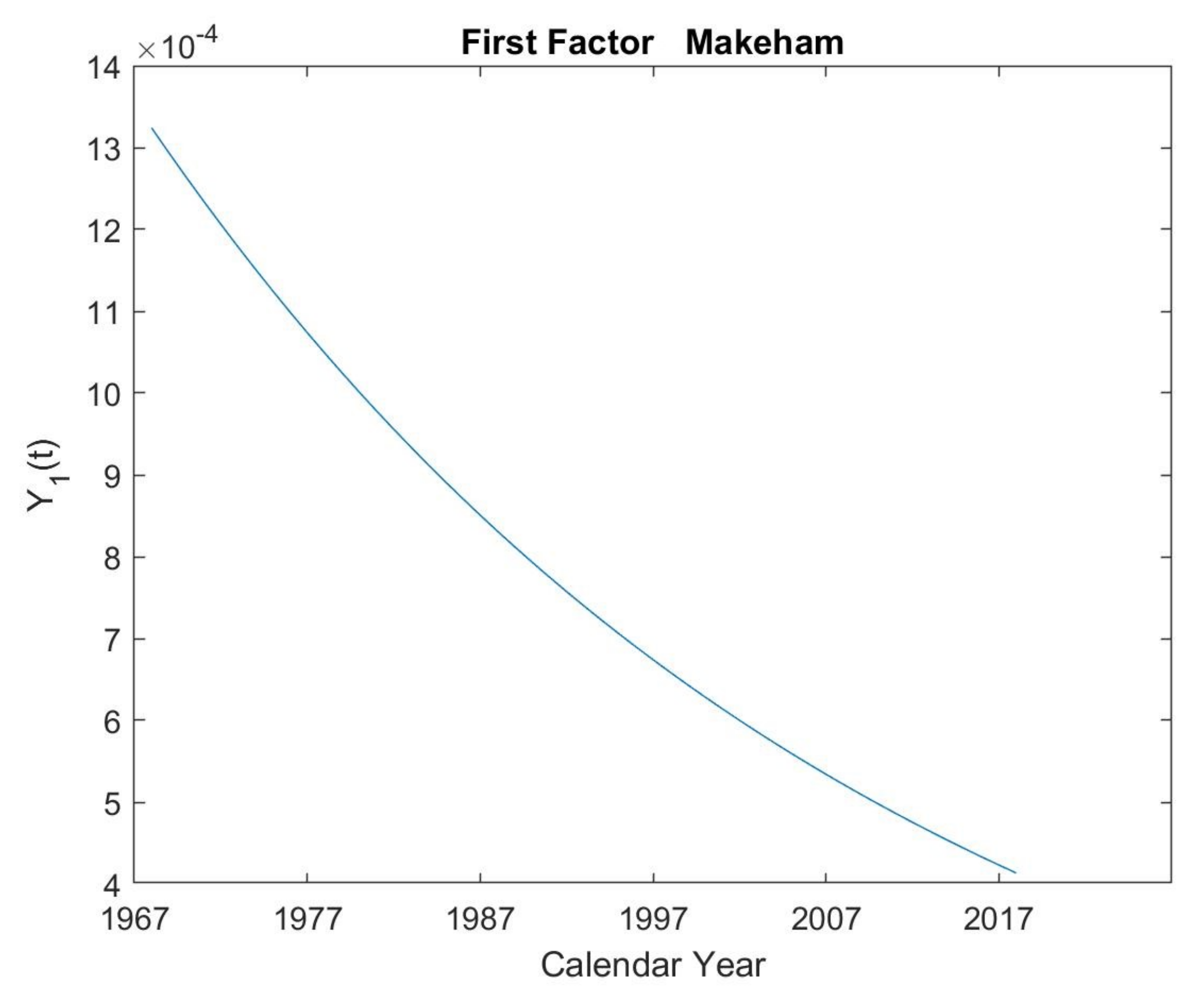
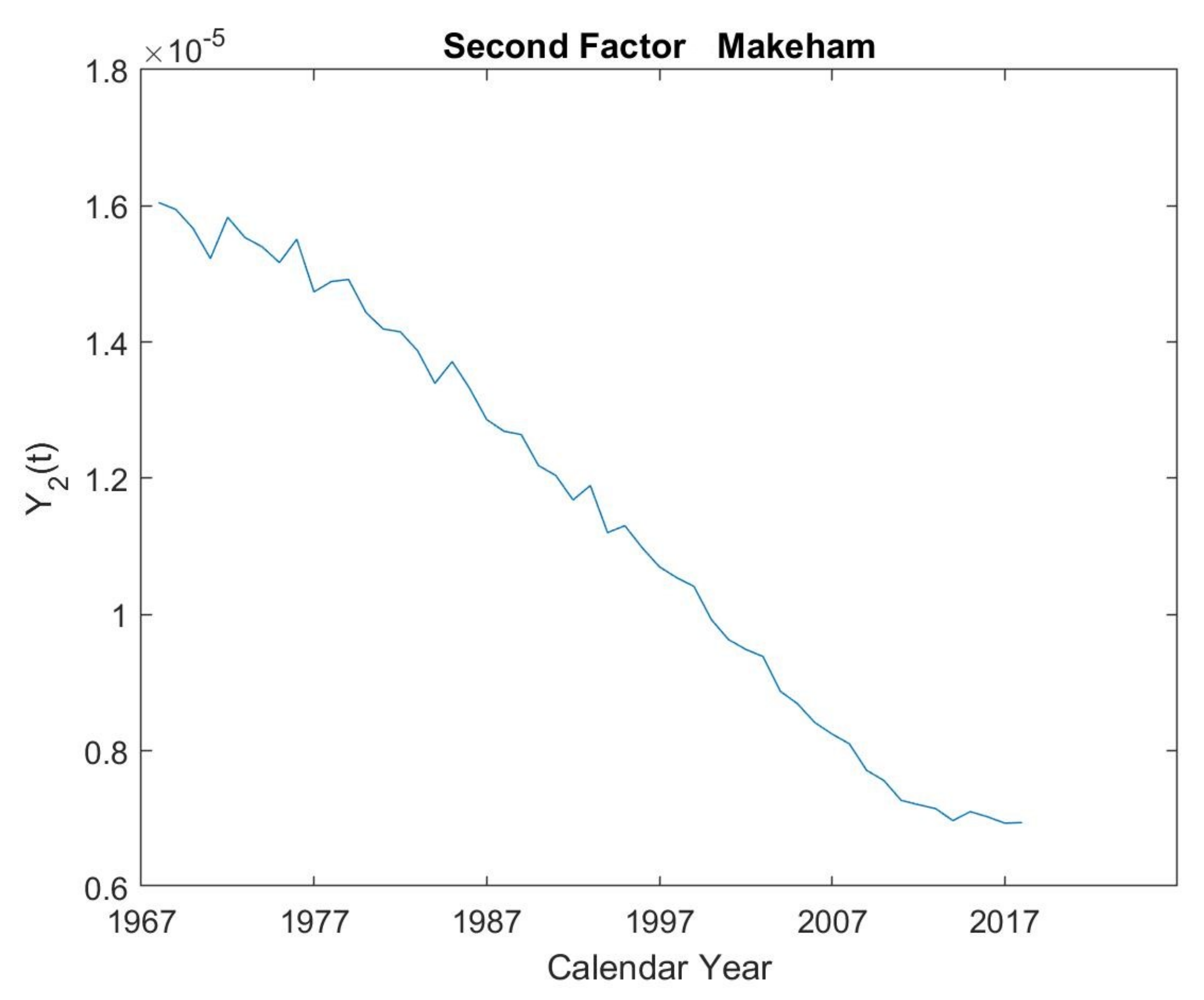
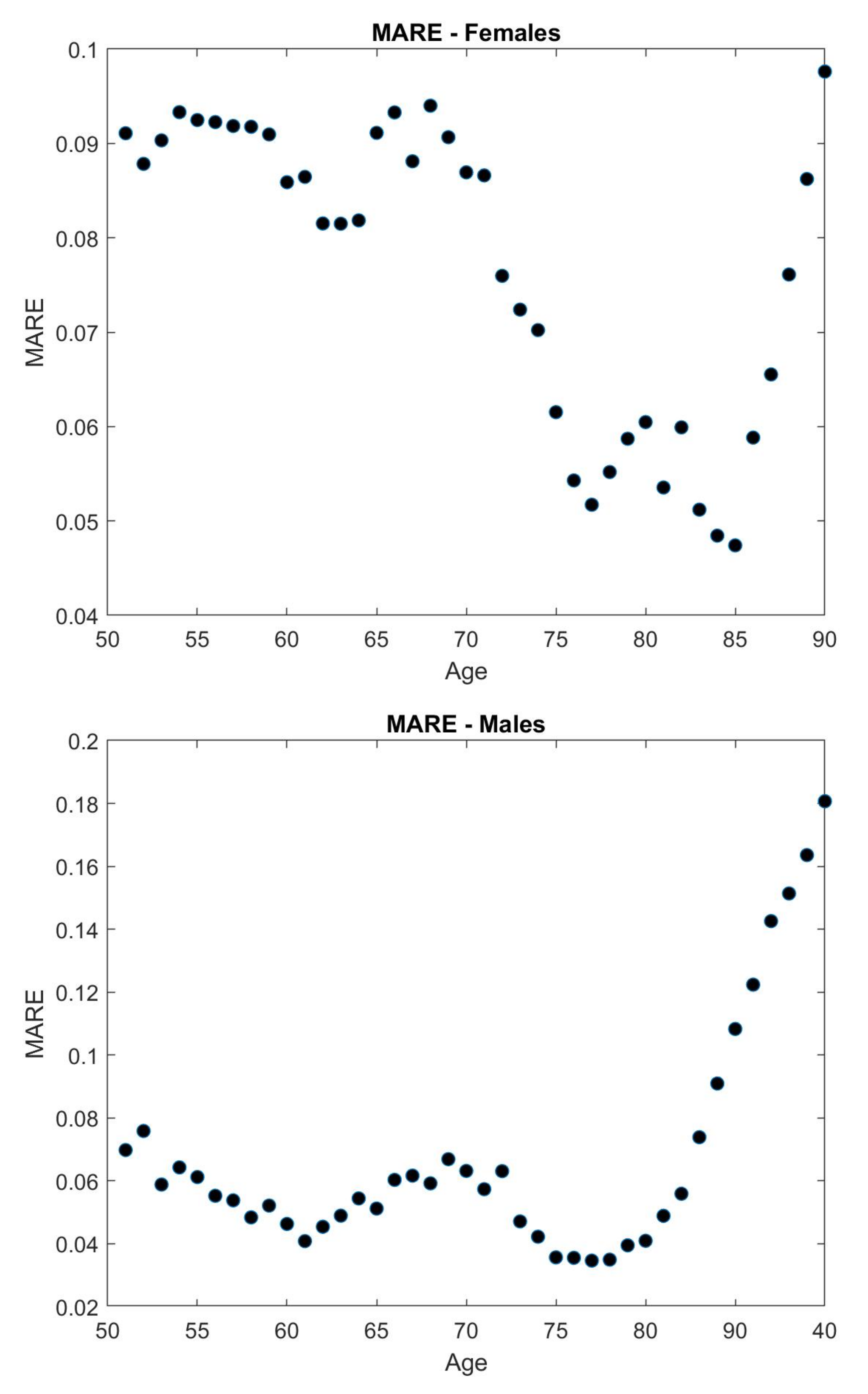
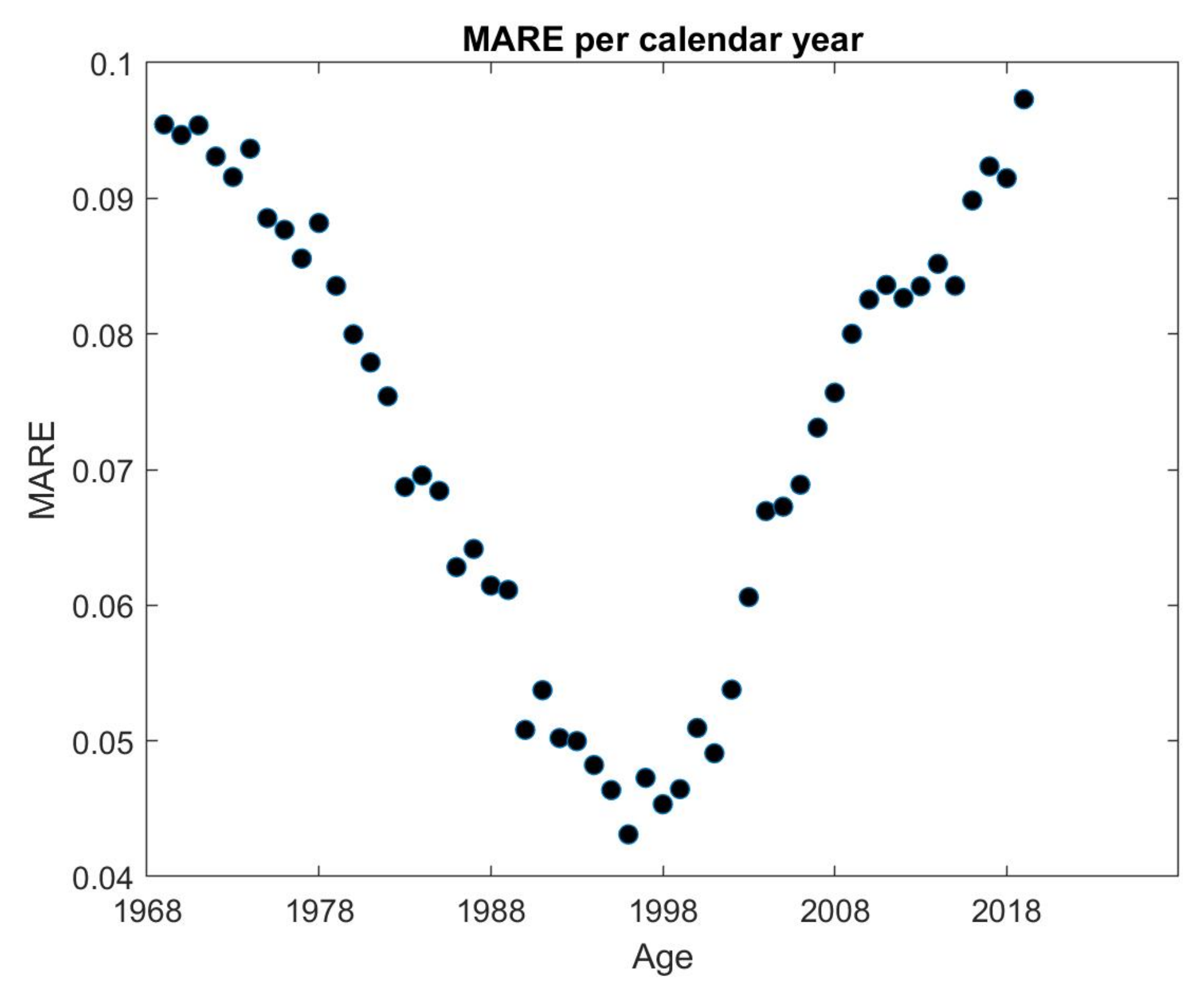
5.1. First Makeham’s Multi-Population Law

We estimate the following model, where $j=1,2$ denote the male and female UK population, respectively:

$${\mu }_{x+t}^j\left(t\right):=Y_1\left(t\right)+{\left({\gamma }^j\right)}^{x+t}{Y}_2\left(t\right).$$

In this case, ${\mathit{g}}^j(x+t,t,x):=[1,{\left({\gamma }^j\right)}^{x+t}]$, with $\mathit{Y}\in {\mathbb{R}}^2$. The model has two factors, which are the same across the populations. Indeed, we dropped dependence on j above. The coefficients $\alpha (·)$ and $\beta {(·)}^j=[{\beta }_1^j,{\beta }_2^j]$ can thus be obtained solving the following ODE system:

$${\dot{\alpha }}^j=-\mathit{A}\mathit{\theta }·{\mathit{\beta }}^j,{\dot{\mathit{\beta }}}^j={[1,{\left({\gamma }^j\right)}^{x+t}]}^{\prime }+{\left(\mathit{A}\right)}^{{}^{\prime }}{\mathit{\beta }}^j-{\left[\frac{1}{2}{\left({\beta }_1^j\right)}^2{\sigma }_1^2,\frac{1}{2}{\left({\beta }_2^j\right)}^2{\sigma }_2^2\right]}^{{}^{\prime }},$$

with final conditions ${\alpha }^j(x,T,T)=0$ and ${\mathit{\beta }}^j(x,T,T)=\mathbf{0}$.

While affected by the same factors, they respond differently to the second factor. It is the only parameter ${\gamma }^j$ that shapes the mortality–age relation for the different populations. Indeed, though very parsimonious, this specification is not rich enough to capture well the complexity of the whole mortality curve. We restrict our application to older ages only, ranging from 50 to 89.

Table 1. This table collects the optimal parameters for our model. For each population, the “common” column collects the parameters relative to the factor processes and the measurement variance–covariance matrix s. The other two columns collect the parameters relative to the response functions of the two populations of males and females.

Maximized Log-Likelihood	22,409	Number of Parameters	9
Optimal Parameters
Common		Males		Females
Parameter	Value	Parameter	Value	Parameter	Value
$a_1$	$0.0233$	${\gamma }^m$	0.1153	${\gamma }^f$	0.0944
$a_2$	$0.0111$
${\sigma }_1$	$2.87\times {10}^{-7}$
${\sigma }_2$	0.0109
${\theta }_1$	0.0014
${\theta }_2$	$2.37\times {10}^{-6}$
s	0.1076

reports the estimated parameters. The population-specific parameter, which captures the steepness of the exponential increase in mortality at old ages captured by Makeham’s mortality law is not unexpectedly higher for UK males (0.1153) than for females (0.0944).

Figure 1 displays the evolution of the values of the latent factors in time. The first factor, which acts as a baseline mortality intensity level, is estimated to decline rather smoothly over time. Notice that its initial value is higher than the long-term estimated average ${\theta }_1$ (0.0014). This parameter can be interpreted as the estimated biological limit which the value of the factor can tend to. The speed of mean reversion $a_1$ (0.0233) can be interpreted as the speed at which the mortality baseline level tends to converge to such long-term value. The second factor, which interacts with age to reproduce the exponential increase of mortality at older ages, also declines. Its volatility is higher because it influences mortality at older ages, reflecting the well-known fact that higher uncertainty surrounds older age mortality improvements. The current values of the factors (i.e., the estimates for the last calendar year) are still far from their long-term averages. Taking into account their exponential decay, we expect the current values ($4\times {10}^{-3}$ and $6\times {10}^{-6}$ respectively) to halve in approximately 173 years, and 115,524 years respectively, and thus still be above their long-term average. The model produces a good fit of the mortality surface, despite its very simple form. Figure 2 reports the Mean Absolute Relative Errors of the single female and male ages (averaged over calendar years):

$$MARE(x,j)=\frac{1}{T}\sum _{t=1}^T\left|\frac{{\widehat{q}}_x^j\left(t\right)-q_x^j\left(t\right)}{q_x^j\left(t\right)}\right|,$$

and of each calendar year (averaged over all the observations):

$$MARE\left(t\right)=\frac{1}{p}\sum _{i=1}^p\left|\frac{{\widehat{q}}_i\left(t\right)-q_i\left(t\right)}{q_i\left(t\right)}\right|,$$

where $\widehat{q}$ denotes the fitted one-year death probability. The model performance is good, given that 4080 observations are fitted with only nine parameters. Average MARE is 7.22%, and it is lower than 10% for almost all ages, apart from older males. This is in line with the two-factor model performance in [1], despite our two-population fit. Only older male figures seem to be more problematic to fit. Performance may be improved assuming that one state process (for instance, the first factor) differs across the two populations.

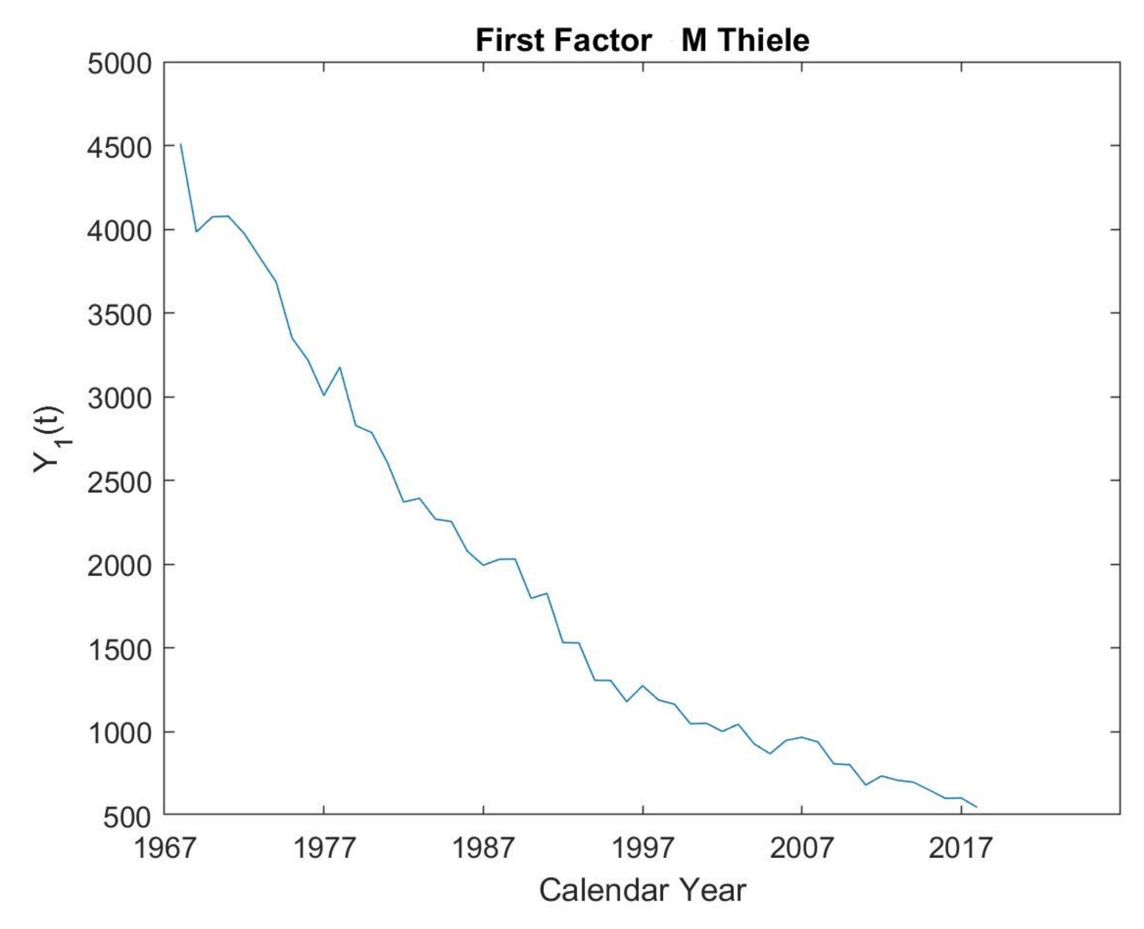
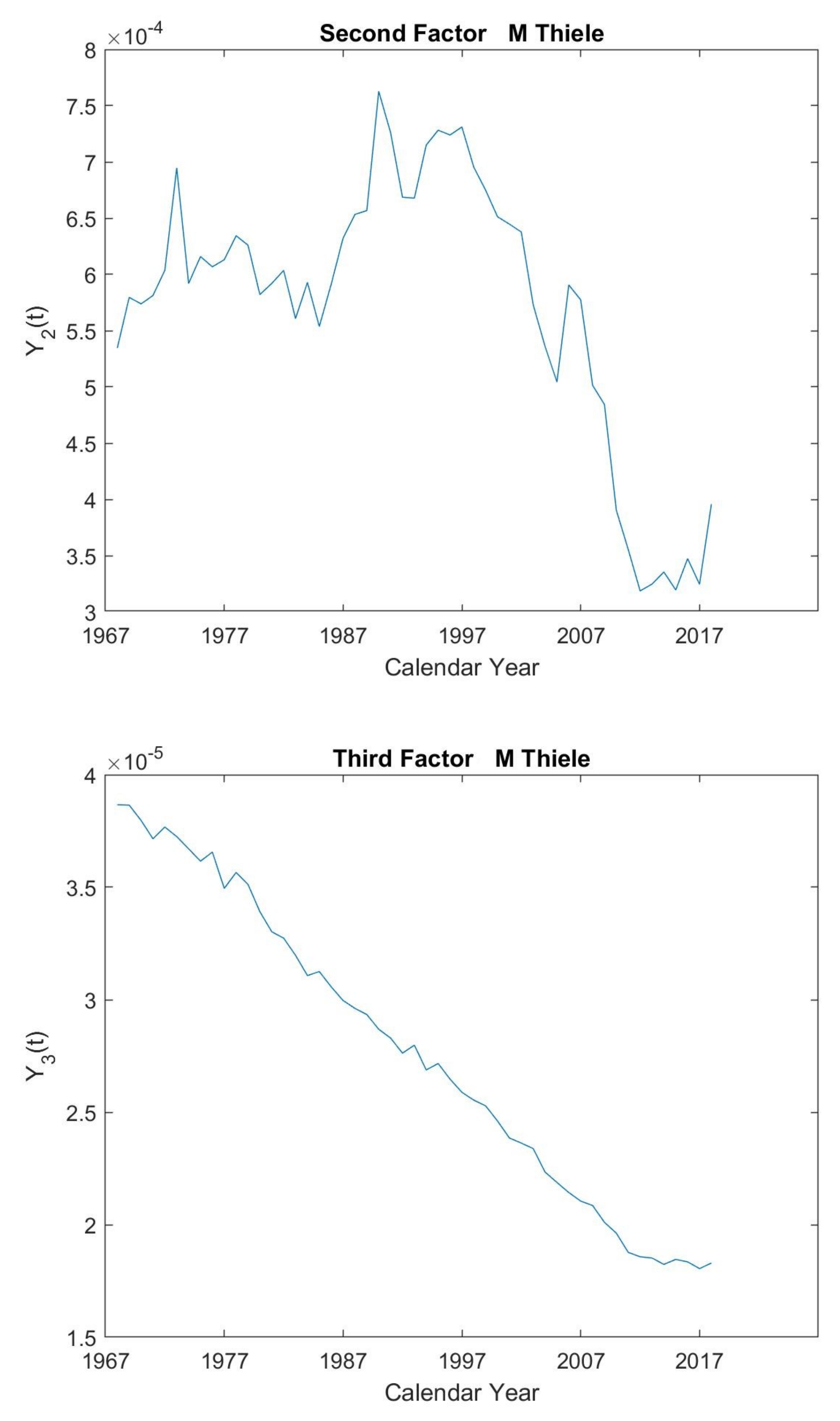
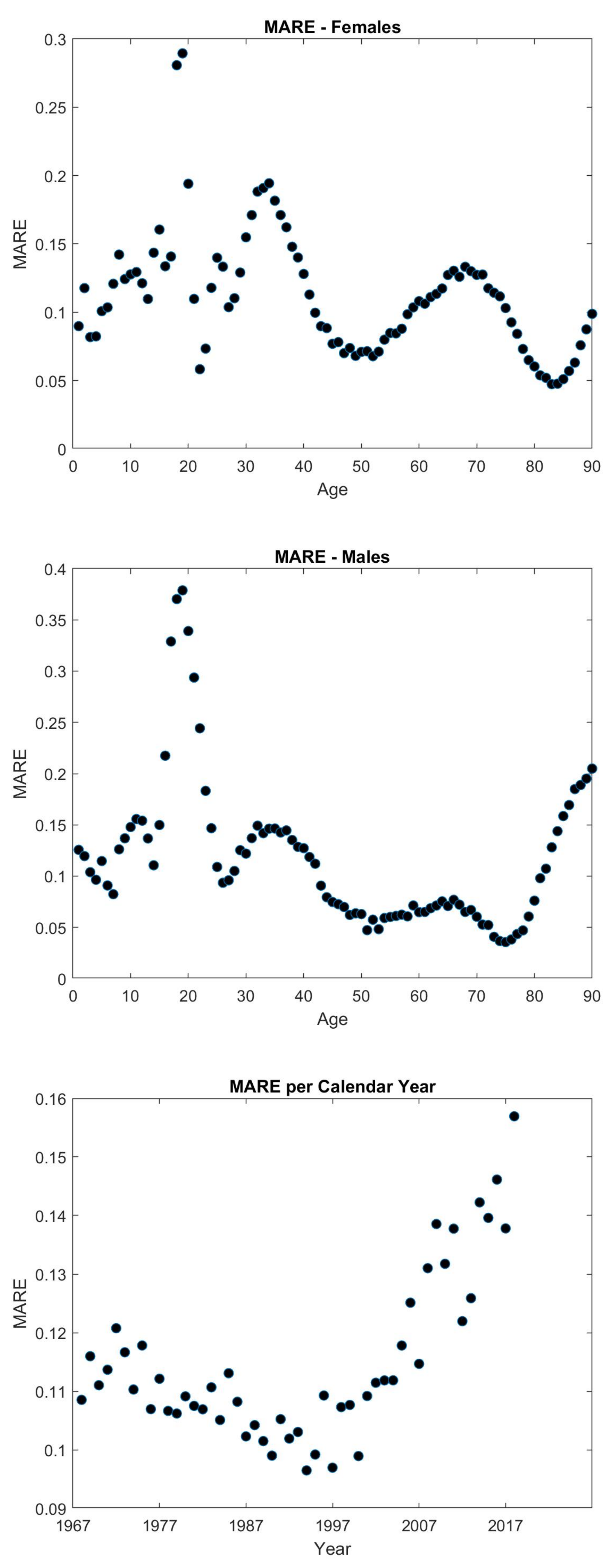
5.2. Modified Thiele’s Law

We estimate the following model, where $j=1,2$ denote the male and female UK population, respectively:

$${\mu }_{x+t}^j\left(t\right):=Y_1\left(t\right)e^{-{\gamma }_1^j{(x+t)}^{\frac{1}{{\gamma }_2^j}}}+Y_2\left(t\right)e^{-{\gamma }_3^j{(x+t-{\gamma }_4^j)}^2}+Y_3\left(t\right){\left({\gamma }_5^j\right)}^{x+t}.$$

In this case, ${\mathit{g}}^j(x+t,t,x):=[e^{-{\gamma }_1^j{(x+t)}^{\frac{1}{{\gamma }_2^j}}},e^{-{\gamma }_3^j{(x+t-{\gamma }_4^j)}^2},{\left({\gamma }_5^j\right)}^{x+t}]$ and $\mathit{Y}\in {\mathbb{R}}^3$. This is a 3-factor model, where factors are the same across the populations. The coefficients $\alpha (·)$ and $\mathit{\beta }{(·)}^j=[{\beta }_1^j,{\beta }_2^j,{\beta }_3^j]$ can be obtained solving the system of ODEs:

$${\dot{\alpha }}^j=-\mathit{A}\mathit{\theta }·{\mathit{\beta }}^j,{\dot{\mathit{\beta }}}^j={[e^{-{{\gamma }_1}^j{(x+t)}^{\frac{1}{{\gamma }_2^j}}},e^{-{\gamma }_3^j{(x+t-{{\gamma }_4}^j)}^2},{{{\gamma }_5}^j}^{x+t}]}^{\prime }+{\mathit{A}}^{{}^{\prime }}{\mathit{\beta }}^j-{\left[\frac{1}{2}{\left({\beta }_1^j\right)}^2{\sigma }_1^2,\frac{1}{2}{\left({\beta }_2^j\right)}^2{\sigma }_2^2,\frac{1}{2}{\left({\beta }_3^j\right)}^2{\sigma }_3^2\right]}^{{}^{\prime }},$$

with final conditions ${\alpha }^j(x,T,T)=0$ and ${\mathit{\beta }}^j(x,T,T)=\mathbf{0}$.

Table 2. This table collects the optimal parameters for our model and is divided in two panels, one for each population. For each population, the ”common” column collects the parameters relative to the factor processes and the measurement variance covariance matrix s. The other two columns collect the parameters relative to the response functions of the two sub-populations of males and females.

Maximized log-Likelihood	65,464	Number of Parameters	20
Optimal Parameters
Common		Males		Females
Parameter	Value	Parameter	Value	Parameter	Value
$a_1$	$2.95\times {10}^{-18}$	${\gamma }_1^m$	$14.8170$	${\gamma }_1^f$	14.4989
$a_2$	$6.40\times {10}^{-6}$	${\gamma }_2^m$	15.8046	${\gamma }_2^f$	15.0810
$a_3$	$2.76\times {10}^{-16}$	${\gamma }_3^m$	0.0048	${\gamma }_3^f$	0.0229
${\sigma }_1$	$0.8521$	${\gamma }_4^m$	88.2853	${\gamma }_4^f$	23.1866
${\sigma }_2$	$2.21\times {10}^{-6}$	${\gamma }_5^m$	0.0944	${\gamma }_5^f$	0.1016
${\sigma }_3$	$2.10\times {10}^{-13}$
${\theta }_1$	88.8547
${\theta }_2$	$2.08\times {10}^{-8}$
${\theta }_3$	$5.32\times {10}^{-7}$
s	0.1496

reports the estimated parameters.

The factors have a constantly decreasing trend in time, apart from the second factor, which decreases over the last 15 calendar years only as depicted by Figure 3 (see Table 1). The first and the third factors decline very fast until the 2000s, to depict the extraordinary improvements in infant mortality and mortality at older ages. As for the Makeham’s law case, the factors are still way above their long-term averages $\theta$ and thus we expect further improvements of mortality in the long-run. Such long-term averages are very important for long-run projections of mortality rates. In unreported estimations, we test the changes of the values of these parameters to slight changes in the estimation time window, finding reasonable stability.

In our estimation procedure, we have not constrained the value of the parameter that controls the age which is mostly affected by the second factor. Thus, the factor affects the different populations differently. For example, it influences female mortality at young adult ages to help to address the accident hump (${\gamma }_4^f=23.1866$). For males, it instead adds up to the third factor in influencing mortality at older ages (${\gamma }_4^m=88.2853$). As Figure 4 shows, the model’s fit is very good for both female and male populations, with an average MARE across all observations of $11.47\%$. The first factor helps capture the infant mortality spike at age 0. Mortality at young adult ages and at older ages is slightly more difficult to capture for males, for which MARE is above the average between ages 18 and 23. Between ages 40 and 70, the curve’s fit is better for males than females.

6. Conclusions

In this paper, we have focused on a stochastic and multi-population extension of traditional actuarial mortality laws. We place ourselves within the setup introduced by [2]. The mortality intensities of all (or a large set of) the ages of multiple populations are modeled within the affine framework as functions of population-specific parameters, which shape the age dependence and some unobservable factors that describe the evolution of mortality trends over time. Here, these latent factors are modeled as square-root processes and describe the evolution of mortality trends over time. The estimation procedure for such models entails dealing with a non-Gaussian state-space model. In this case, estimation via Kalman filter still provides us with the optimal linear state estimator. However, this may be sub-optimal due to the non-linearities introduced by the state-vector process density. We followed [7] and applied a Quasi-Linear Kalman Filter algorithm that approximates the state process transition density to a Gaussian density truncated at 0 with the same conditional first two moments. Although approximate, the procedure was proven accurate enough in a similar setup when fitting multi-factor CIR models for interest rates. Relative to previous similar multi-population models, the mortality intensities are thus guaranteed to be non-negative. This is indeed an advantage relative to Gaussian models, especially when the model needs to be applied to forecast intensities over long time periods. Obviously, this can be important when dealing with the pricing of long-term liabilities, such as annuities, or with risk management for pension funds. Inspired by the Makeham and the Thiele laws, our application provides the calibration of two stochastic multi-population mortality laws to the UK populations of males and females mortality rates jointly from 1968 to 2017. The models are parsimonious and are shown to provide a good fit of the mortality surface over time.

References

1. Schrager, D.F. Affine stochastic mortality. Insur. Math. Econom. 2006, 38, 81–97. [Google Scholar] [CrossRef] [Green Version]
2. Jevtić, P.; Regis, L. A continuous-time stochastic model for the mortality surface of multiple populations. Insur. Math. Econom. 2019, 88, 181–195. [Google Scholar] [CrossRef] [Green Version]
3. Jevtić, P.; Luciano, E.; Vigna, E. Mortality surface by means of continuous time cohort models. Insur. Math. Econom. 2013, 53, 122–133. [Google Scholar] [CrossRef]
4. Blackburn, C.; Sherris, M. Consistent dynamic affine mortality models for longevity risk applications. Insur. Math. Econom. 2013, 53, 64–73. [Google Scholar] [CrossRef]
5. De Rosa, C.; Luciano, E.; Regis, L. Geographical diversification and longevity risk mitigation in annuity portfolios. ASTIN Bull. J. IAA 2021, 51, 375–410. [Google Scholar] [CrossRef]
6. Cox, J.C.; Ingersoll, J.E., Jr.; Ross, S.A. An intertemporal general equilibrium model of asset prices. Econometrica 1985, 53, 363–384. [Google Scholar] [CrossRef] [Green Version]
7. Chen, R.R.; Scott, L. Multi-factor Cox-Ingersoll-Ross models of the term structure: Estimates and tests from a Kalman filter model. J. Real Estate Financ. Econ. 2003, 27, 143–172. [Google Scholar] [CrossRef]
8. Simon, D. Optimal State Estimation: Kalman, H Infinity, and Nonlinear Approaches; John Wiley & Sons: Hoboken, NJ, USA, 2006. [Google Scholar]
9. Pitacco, E.; Denuit, M.; Haberman, S. Modelling Longevity Dynamics for Pensions and Annuity Business; Oxford University Press: Oxford, UK, 2009. [Google Scholar]
10. Milevsky, M.A.; Promislow, S.D. Mortality Derivatives and the Option to Annuitise. Insur. Math. Econom. 2001, 29, 299–318. [Google Scholar] [CrossRef]
11. Lando, D. On Cox processes and credit risky securities. Rev. Deriv. Res. 1998, 2, 99–120. [Google Scholar] [CrossRef]
12. Duffie, D.; Pan, J.; Singleton, K. Transform analysis and asset pricing for affine jump-diffusions. Econometrica 2000, 68, 1343–1376. [Google Scholar] [CrossRef] [Green Version]
13. Filipović, D. Term-Structure Models: A Graduate Course, 1st ed.; Springer: Berlin/Heidelberg, Germany, 2009. [Google Scholar]
14. Duffie, D.; Kan, R. A yield-factor model of interest rates. Math. Financ. 1996, 6, 379–406. [Google Scholar] [CrossRef] [Green Version]
15. Raol, J.R. Multi-Sensor Data Fusion with MATLAB®; CRC Press: Boca Raton, FL, USA, 2009. [Google Scholar]
16. Duan, J.C.; Simonato, J.G. Estimating and testing exponential-affine term structure models by Kalman filter. Rev. Quant. Financ. Account. 1999, 13, 111–135. [Google Scholar] [CrossRef]
17. Koopman, S.J.; Durbin, J. Fast filtering and smoothing for multivariate state space models. J. Time Ser. Anal. 2000, 21, 281–296. [Google Scholar] [CrossRef]
18. Kitagawa, G. Monte Carlo filter and smoother for non-Gaussian nonlinear state space models. J. Comput. Graph. Stat. 1996, 5, 1–25. [Google Scholar] [CrossRef]
19. De Rossi, G. Maximum likelihood estimation of the Cox–Ingersoll–Ross model using particle filters. Comput. Econ. 2010, 36, 1–16. [Google Scholar] [CrossRef]
20. Jong, F.d. Time series and cross-section information in affine term-structure models. J. Bus. Econ. Stat. 2000, 18, 300–314. [Google Scholar] [CrossRef] [Green Version]
21. Chen, R.R.; Scott, L. Maximum likelihood estimation for a multifactor equilibrium model of the term structure of interest rates. J. Fixed Income 1993, 3, 14–31. [Google Scholar] [CrossRef]
22. Storn, R.; Price, K. Differential evolution—A simple and efficient heuristic for global optimization over continuous spaces. J. Glob. Optim. 1997, 11, 341–359. [Google Scholar] [CrossRef]
Figure 1. The figure plots the values of the two factors, Y1, Y2.
Mathematics 09 02402 g001aMathematics 09 02402 g001b
Figure 2. The figures plot the values of the MARE for female and male ages and averaged over calendar years.
Mathematics 09 02402 g002aMathematics 09 02402 g002b
Figure 3. The figure plots the values of the three factors, Y1, Y2, Y3.
Mathematics 09 02402 g003aMathematics 09 02402 g003b
Figure 4. The figure plots the values of the MARE for the ages of female and male participants and averaged over calendar years.
Mathematics 09 02402 g004