A Posteriori Fractional Tikhonov Regularization Method for the Problem of Analytic Continuation

Abstract

In this paper, the numerical analytic continuation problem is addressed and a fractional Tikhonov regularization method is proposed. The fractional Tikhonov regularization not only overcomes the difficulty of analyzing the ill-posedness of the continuation problem but also obtains a more accurate numerical result for the discontinuity of solution. This article mainly discusses the a posteriori parameter selection rules of the fractional Tikhonov regularization method, and an error estimate is given. Furthermore, numerical results show that the proposed method works effectively.

1. Introduction

The problem of analytic continuation arises in many fields [1,2,3]. For instance, medical imaging [4,5], the inversion of Laplace transform [6], inverse scattering problems [7], and so on. The analytical continuation problem is described as follows [8].

Problem 1.

Let

$${\Omega }_{*}:=\{z=x+iy\in \mathbb{C}|x\in \mathbb{R},0<y\le a,a>0\}$$

be the strip domain in complex plane $\mathbb{C}$, where i is the imaginary unit and a is a positive constant. The function $h(z)=h(x+iy)$ is an analytic function in ${\Omega }_{*}$. When $y=0$, ${h(z)|}_{y=0}=h(x)\in L^2(\mathbb{R})$. It is easy to show that the data $h(z)$ are only given on the real axis, so we want extend $h(z)$ analytically from these data to the whole domain ${\Omega }_{*}$ and determine the value of function $h(z)$ on ${\Omega }_{*}$ by using data $h(x)$ for $0<y\le a$.

Numerical analytic continuation is a severely ill-posed problem [9]. In order to calculate a stable numerical solution, a certain regularization technique is required. In [8], the authors used the modified Tikhonov regularization method to solve this problem. Recently, this problem has been studied by many researchers with different regularization methods [10,11,12,13]. In [14,15], the authors give an optimal filtering method and a wavelet method for stable analytic continuation, respectively. In [16], Xiong gives the conditional stability estimate for the analytical continuation problem and provides a generalized Tikhonov regularization method. Landweber-type iteration and modified Lavrentiev iterative regularization method are provided by Cheng and Xiong in [17,18]. In [19], the authors used fractional Landweber iterative regularization method to solve this problem, which greatly reduces the number of iteration steps.

In this study, in order to better reconstruct the characteristics of exact solutions, we propose a fractional Tikhonov regularization method to solve Problem 1. The fractional Tikhonov regularization method was first proposed by Klann [20], which is based on the classic Tikhonov regularization method; regarding the Tikhonov’s variational approach, we can refer to the work of A.N. Tikhonov et al. [21]. Related research on fractional regularization methods can refer to the literature [22,23,24,25,26,27,28,29]. The fractional Tikhonov method with the a priori parameter for the same analytic continuation problem has been researched by [30]. As far as we know, there are very few works related to the a posteriori fractional regularization methods, and most of the research on the fractional regularization methods are in the case of compact operators. However, the a priori regularization parameter selection method is based on the smoothness condition of the solution. Although it is convenient for theoretical analysis, it is difficult to verify. Therefore, in practical problems, the a posteriori regularization parameter selection method is more widely used based on the error level information and the error data themselves. Based on the above reasons, we will use the a posteriori fractional Tikhonov regularization method to study the analytical continuation problem mentioned at the beginning of the article. Let

$$\widehat{h}(\xi )=\frac{1}{\sqrt{2\pi }}{\int }_{-\infty }^{\infty }{e}^{-ix\xi }h(x)dx,i=\sqrt{-1},$$

(1)

be the Fourier transform of the function $h(x)\in L^2(\mathbb{R})$; $\xi \in \mathbb{R}$, the corresponding inverse Fourier transform of the function $\widehat{h}(\xi )$, is given by

$$h(x)=\frac{1}{\sqrt{2\pi }}{\int }_{-\infty }^{\infty }{e}^{ix\xi }\widehat{h}(\xi )d\xi .$$

(2)

In this paper, $\parallel ·\parallel$ denotes the $L^2(\mathbb{R})$ norm; according to the Parseval formula, it has the following form:

$$\parallel h\parallel =({\int }_{-\infty }^{\infty }|\widehat{h}(\xi ){{|}^{2}d\xi )}^{\frac{1}{2}},$$

(3)

According to the inverse Fourier transform, we have

$$h(z)=h(x+iy)=\frac{1}{\sqrt{2\pi }}{\int }_{-\infty }^{\infty }{e}^{i(x+iy)\xi }\widehat{h}(\xi )d\xi =\frac{1}{\sqrt{2\pi }}{\int }_{-\infty }^{\infty }{e}^{ix\xi }{e}^{-y\xi }\widehat{h}(\xi )d\xi .$$

(4)

For simplicity, we denote $\omega (x,y)=h(x+iy)$. Therefore, we can easily obtain the solution to the problem in the frequency domain as follows:

$$\widehat{\omega }(\xi ,y)=e^{-y\xi }\widehat{h}(\xi ).$$

(5)

From (5), we know that the operator equation of the problem is as follows

$$K_y\widehat{\omega }(\xi ,y)=\widehat{h}(\xi ).$$

(6)

where $K_y=e^{y\xi }:L^2(\mathbb{R})\to L^2(\mathbb{R})$ is the self-adjoint multiplication operator.

Note the factor $e^{-y\xi }\to +\infty$ as $\xi \to -\infty$, given a small change in the data $h(\xi )$, the solution $\widehat{\omega }(\xi ,y)$ will have a huge change through the error factor $e^{-y\xi }$. It is easy to see the ill-posedness of Problem 1 is due to the negative high frequencies. Therefore, when $\xi <0$, it is impossible to stably solve the problem using classical methods, it needs to be regularized to calculate a stable numerical solution. We construct the regularization solution of Problem 1 in the frequency domain according to the fractional Tikhonov regularization method given in reference [29] as follows

$${\widehat{\omega }}_{\mu }^{\delta }(\xi ,y)=\frac{e^{-y\xi }}{1+\mu e^{-2\gamma y\xi }}{\widehat{h}}^{\delta }(\xi ),\frac{1}{2}<\gamma \le 1.$$

(7)

Compared with expression (5), the filter factor $\frac{1}{1+\mu e^{-2\gamma y\xi }}$ in (7) attenuates the high-frequency part of understanding, and we can use another better decay filter $\frac{1}{1+\mu e^{-2\gamma a\xi }}$ to replace the original one and we can get better convergence results. Therefore, we can obtain a new regularization solution

$${\widehat{\omega }}_{\mu }^{\delta }(\xi ,y)=\frac{e^{-y\xi }}{1+\mu e^{-2\gamma a\xi }}{\widehat{h}}^{\delta }(\xi ),\frac{1}{2}<\gamma \le 1,$$

(8)

where $\mu >0$ plays the role of regularization parameter. We call $\gamma$ the fractional parameter; when $\gamma =\frac{1}{2}$, we obtain the quasi-boundary value method, and when $\gamma =1$, it expresses the classic Tikhonov method. $\frac{1}{2}<\gamma <1$ is used for the fractional Tikhonov regularization methodBecause measurement errors exist in the data function $h(x)$, we assume the exact data $h(x)$ and the measured data $h^{\delta }(x)$ both belong to $L^2(\mathbb{R})$ and satisfy

$$\parallel h^{\delta }(·)-h(·)\parallel \le \delta ,$$

(9)

where $\delta >0$ denotes the noise level. Then we extend $h(z)$ analytically from these data to the whole domain $\Omega$ such that

$$\parallel \omega (·,a)\parallel =\parallel \widehat{\omega }(·,a)\parallel \le M,$$

(10)

where M is a fixed positive constant.

The article is organized as follows. In Section 2, we consider the a posteriori parameter choice rule for fractional Tikhonov regularization method and give a Hölder-type error estimate. In Section 3, we provide some numerical examples to show the validity of the proposed fractional Tikhonov regularization method. Finally, we give concluding remarks in Section 4.

2. An A Posteriori Regularization Parameter Choice Rule for the Fractional Tikhonov Method and the Convergence Estimate

In this section, we apply the fractional Tikhonov method with posterior parameter selection rules to the analytical continuation problem and provide the specific rate of convergence for the regularized approximation. We use the Morozov’s discrepancy principle to choose the regularization parameter $\mu$; for Morozov’s discrepancy principle, please refer to Reference [31]. We choose the regularization parameters $\mu$ to satisfy

$$\parallel K_y{\widehat{\omega }}_{\mu }^{\delta }(\xi ,y)-{\widehat{h}}^{\delta }(\xi )\parallel =\tau \delta ,$$

(11)

where $\frac{1}{2}<\gamma \le 1,\tau >1$ is a constant and $\mu >0$ is a regularization parameter.

In order to prove our main result, we give the following auxiliary lemmas.

Lemma 1

([32]). Let $0<m<n$, $k>0$; then

$$\underset{k>0}{sup}\frac{e^{km}}{1+\mu e^{kn}}\le {\mu }^{-\frac{m}{n}}.$$

(12)

Lemma 2.

Set $d(\mu )=\parallel K_y{\widehat{\omega }}_{\mu }^{\delta }(\xi ,y)-{\widehat{h}}^{\delta }(\xi )\parallel$. If $0<\delta <\parallel {\widehat{h}}^{\delta }\parallel$, then the following hold:

(a) 

$d(\mu )$ is a continuous function;

(b) 

$li{m}_{\mu \to 0}d(\mu )=0$;

(c) 

$li{m}_{\mu \to \infty }d(\mu )={\parallel {\widehat{h}}^{\delta }\parallel }_{L^2(\mathbb{R})}$;

(d) 

$d(\mu )$ is a strictly increasing function over $(0,\infty )$.

Proof. 

From (11), we have

$$d(\mu )=\parallel \frac{\mu e^{-2\gamma a\xi }}{1+\mu e^{-2\gamma a\xi }}{\widehat{h}}^{\delta }(\xi )\parallel .$$

(13)

The above result can be easily obtained by the expression of $d(\mu )$. □

Remark 1.

From Lemma 2, we know that there exists a unique solution μ satisfying Equation (11).

Lemma 3. 

If μ is the solution of Equation (11), we also obtain the following inequality:

$${\mu }^{-\frac{1}{2\gamma }}\le \frac{M}{(\tau -1)\delta }.$$

(14)

Proof. 

From (11) and Lemma 2, we obtain

$$\begin{array}{cc}\hfill \tau \delta & =\parallel \frac{\mu e^{-2\gamma a\xi }}{1+\mu e^{-2\gamma a\xi }}{\widehat{h}}^{\delta }(\xi )\parallel \hfill \\ \hfill & \le \parallel \frac{\mu e^{-2\gamma a\xi }}{1+\mu e^{-2\gamma a\xi }}({\widehat{h}}^{\delta }(\xi )-\widehat{h}(\xi ))\parallel +\parallel \frac{\mu e^{-2\gamma a\xi }}{1+\mu e^{-2\gamma a\xi }}\widehat{h}(\xi )\parallel .\hfill \end{array}$$

(15)

From the noise assumptiona priori condition (9) and the a priori condition (10), there holds

$$\begin{array}{cc}\hfill \tau \delta & \le \delta +\mu ·\parallel \frac{e^{-(2\gamma -1)a\xi }}{1+\mu e^{-2\gamma a\xi }}{e}^{-a\xi }\widehat{h}(\xi )\parallel \hfill \\ \hfill & \le \delta +\mu ·M·\underset{\xi <0}{sup}\frac{e^{-(2\gamma -1)a\xi }}{1+\mu e^{-2\gamma a\xi }}.\hfill \end{array}$$

(16)

According to Lemma 1, we obtain

$$\tau \delta \le \delta +{\mu }^{\frac{1}{2\gamma }}M.$$

So

$$\begin{array}{c}\hfill {\mu }^{-\frac{1}{2\gamma }}\le \frac{M}{(\tau -1)\delta }.\end{array}$$

□

Lemma 4. 

Set

$${\varphi }_{\mu }^{\delta }(·,y):=\widehat{\omega }(\xi ,y)-{\widehat{\omega }}_{\mu }^{\delta }(\xi ,y);$$

(17)

then the following inequality holds

$$\parallel {\varphi }_{\mu }^{\delta }(·,y)\parallel \le \parallel {\varphi }_{\mu }^{\delta }{(·,a)\parallel }^{\frac{y}{a}}{\parallel {\varphi }_{\mu }^{\delta }(·,0)\parallel }^{1-\frac{y}{a}}.$$

(18)

Proof. 

By (17), it is easy to see that

$${\varphi }_{\mu }^{\delta }(·,y)=e^{-y\xi }\widehat{h}(\xi )-\frac{e^{-y\xi }}{1+\mu e^{-2\gamma a\xi }}\widehat{h^{\delta }}(\xi ),$$

then

$${\varphi }_{\mu }^{\delta }(·,0)=\widehat{h}(\xi )-\frac{1}{1+\mu e^{-2\gamma a\xi }}{\widehat{h}}^{\delta }(\xi ),$$

$${\varphi }_{\mu }^{\delta }(·,a)=e^{-a\xi }\widehat{h}(\xi )-\frac{e^{-a\xi }}{1+\mu |e^{-a\xi }{|}^{2\gamma }}\widehat{h^{\delta }}(\xi ).$$

By the Hölder inequality, we obtain

$$\begin{array}{cc}\hfill \parallel {\varphi }_{\mu }^{\delta }{(·,y)\parallel }^2& ={\int }_{-\infty }^{\infty }{|e^{-y\xi }\widehat{h}(\xi )-\frac{e^{-y\xi }}{1+\mu e^{-2\gamma a\xi }}\widehat{h^{\delta }}(\xi )|}^{2}d\xi \hfill \\ \hfill & ={\int }_{-\infty }^{\infty }{e}^{-2y\xi }{\left({\Theta }_h(\mu ,\xi ,\delta )\right)}^{\frac{2y}{a}}·{\left({\Theta }_h(\mu ,\xi ,\delta )\right)}^{2(1-\frac{y}{a})}d\xi \hfill \\ \hfill & \le {\left({\int }_{-\infty }^{\infty }{(e^{-y\xi })}^{\frac{2a}{y}}{\left({\Theta }_h(\mu ,\xi ,\delta )\right)}^{2}d\xi \right)}^{\frac{y}{a}}·{\left({\int }_{-\infty }^{\infty }{\left({\Theta }_h(\mu ,\xi ,\delta )\right)}^{2}d\xi \right)}^{1-\frac{y}{a}}\hfill \\ \hfill & ={\left({\int }_{-\infty }^{\infty }{e}^{-2a\xi }{\left({\Theta }_h(\mu ,\xi ,\delta )\right)}^{2}d\xi \right)}^{\frac{y}{a}}·{\left({\int }_{-\infty }^{\infty }{\left({\Theta }_h(\mu ,\xi ,\delta )\right)}^{2}d\xi \right)}^{1-\frac{y}{a}}\hfill \\ \hfill & =\parallel {\varphi }_{\mu }^{\delta }{(·,a)\parallel }^{\frac{2y}{a}}{\parallel {\varphi }_{\mu }^{\delta }(·,0)\parallel }^{2(1-\frac{y}{a})},\hfill \end{array}$$

where ${\Theta }_h(\mu ,\xi ,\delta )=\widehat{h}(\xi )-\frac{1}{1+\mu e^{-2\gamma a\xi }}{\widehat{h}}^{\delta }(\xi )$. Thus, we obtain the result. □

Lemma 5. 

The following inequalities holds

$$\parallel {\varphi }_{\mu }^{\delta }(·,0)\parallel \le (\tau +1)\delta ,$$

(19)

$$\parallel {\varphi }_{\mu }^{\delta }(·,a)\parallel \le \frac{\tau E}{\tau -1}.$$

(20)

Proof. 

First we prove (19). Using the triangle inequality and Equation (11), we get

$$\begin{array}{cc}\hfill \parallel {\varphi }_{\mu }^{\delta }(·,0)\parallel & =\parallel \widehat{h}(\xi )-\frac{1}{1+\mu e^{-2\gamma a\xi }}{\widehat{h}}^{\delta }(\xi )\parallel \hfill \\ \hfill & \le \parallel \widehat{h}(\xi )-{\widehat{h}}^{\delta }(\xi )\parallel +\parallel {\widehat{h}}^{\delta }(\xi )-\frac{1}{1+\mu e^{-2\gamma a\xi }}{\widehat{h}}^{\delta }(\xi )\parallel \hfill \\ \hfill & \le (\tau +1)\delta .\hfill \end{array}$$

(21)

Then, we prove (20). Using the triangle inequality, we get

$$\begin{array}{cc}\hfill \parallel {\varphi }_{\mu }^{\delta }(·,a)\parallel & =\parallel e^{-a\xi }\widehat{h}(\xi )-\frac{e^{-a\xi }}{1+\mu e^{-2\gamma a\xi }}{\widehat{h}}^{\delta }(\xi )\parallel \hfill \\ \hfill & \le \parallel e^{-a\xi }\widehat{h}(\xi )-\frac{e^{-a\xi }}{1+\mu e^{-2\gamma a\xi }}\widehat{h}(\xi )\parallel +\parallel \frac{e^{-a\xi }}{1+\mu e^{-2\gamma a\xi }}(\widehat{h}(\xi )-{\widehat{h}}^{\delta }(\xi ))\parallel \hfill \end{array}$$

(22)

By the noise assumption (9) and the a priori condition (10) and Lemma 3, we obtain,

$$\begin{array}{cc}\hfill \parallel {\varphi }_{\mu }^{\delta }(·,a)\parallel & \le \parallel (1-\frac{1}{1+\mu e^{-2\gamma a\xi }})e^{-a\xi }\widehat{h}(\xi )\parallel +\delta \underset{\xi <0}{sup}\frac{e^{-a\xi }}{1+\mu e^{-2\gamma a\xi }}\hfill \\ \hfill & \le M+\delta {\mu }^{-\frac{1}{2\gamma }}\hfill \\ \hfill & \le \frac{\tau M}{\tau -1}.\hfill \end{array}$$

(23)

□

Now we give the main result of our regularization.

Theorem 1. 

Suppose the a priori condition (10) and the noise assumption (9) hold. Let $\omega (·,y)$ be the exact solution, and ${\omega }_{\mu }^{\delta }(·,y)$ be its regularized approximation defined by (7). Choose the solution of Equation (11) as the value of the posterior regularization parameter μ; then we obtain the following error estimate:

$$\parallel {\omega }_{\mu }^{\delta }(·,y)-\omega (·,y)\parallel \le c_1{M}^{\frac{y}{a}}{\delta }^{1-\frac{y}{a}},$$

(24)

where $c_1:={(\frac{\tau }{\tau -1})}^{\frac{y}{a}}{(\tau +1)}^{1-\frac{y}{a}}$.

Proof. 

Using Parseval’s equality and Lemma 4, we know

$$\begin{array}{cc}\hfill \parallel {\omega }_{\mu }^{\delta }(·,y)-\omega (·,y)\parallel & =\parallel {\widehat{\omega }}_{\mu }^{\delta }(\xi ,y)-\widehat{\omega }(\xi ,y)\parallel \hfill \\ \hfill & \le \parallel {\varphi }_{\mu }^{\delta }{(·,a)\parallel }^{\frac{y}{a}}{\parallel {\varphi }_{\mu }^{\delta }(·,0)\parallel }^{1-\frac{y}{a}}.\hfill \end{array}$$

(25)

According to Lemma 5, we have

$$\parallel {\omega }_{\mu }^{\delta }(·,y)-\omega (·,y)\parallel \le {(\frac{\tau M}{\tau -1})}^{\frac{y}{a}}{((\tau +1)\delta )}^{1-\frac{y}{a}}=c_1{M}^{\frac{y}{a}}{\delta }^{1-\frac{y}{a}},$$

where $c_1=(\tau +1){(\frac{\tau }{(\tau +1)(\tau -1)})}^{\frac{y}{a}}$. The proof of Theorem 1 is completed. □

3. Numerical Examples

In this section, we use some numerical examples to verify the effectiveness of the fractional Tikhonov regularization method. The fractional Tikhonov regularization method can be implemented by fast Fourier transform. In these numerical experiments, we always take $a=1$ and fix the domain ${\Omega }_{*}=\{z=x+iy\in \mathbb{C}\mid |x|\le 10,0<y<1\}$. Suppose the vector G and $G(x+iy)$ represent samples from the function $G(x)$ and $\omega (·,y)$; then we can obtain the perturbation data through

$$G^{\delta }=G+\delta ·randn(size(G)).$$

(26)

Here “$randn(·)$” means to generate a set of random numbers that obey the standard normal distribution. The error is given by (Root Mean Square Error ($RMSE$))

$$RMSE=\parallel G^{\delta }{-G\parallel }_{l^2}:=\sqrt{\frac{1}{N+1}\sum _{n=1}^{N+1}{|G^{\delta }(n)-G(n)|}^2}.$$

(27)

In the numerical experiments, we denote the corresponding RMSEs of the real part and imaginary part as $RMS{E}_{Re}$ and $RMS{E}_{Im}$, respectively. We usually choose $N=200$. ${\omega }_{\mu }^{\delta }(·,y)$ represent the regularization solution calculated by the fractional Tikhonov method. We give numerical results under the a posteriori choice rule. The a posteriori parameter $\mu$ is selected by (11). In these experiments, we fix the fractional parameter $\gamma =2/3$ and noise level $\delta =0.01$. In the following numerical examples, we consider problems of [18].

Example 1.

The function

$$h(z)=e^{-z^2}=e^{-{(x+iy)}^2}=e^{y^2-x^2}(cos2xy-isin2xy)$$

is analytic in the domain

$${\Omega }_{*}=\{z=x+iy\in \mathbb{C}\mid x\in \mathbb{R},0<y\le 1\}$$

with $h(z){\mid }_{y=0}=e^{-x^2}\in L^2(\mathbb{R})$, $Reh(z)=e^{y^2-x^2}cos2xy$, $Imh(z)=-e^{y^2-x^2}sin2xy$.

Figure 1 shows the numerical results of the a posteriori parameter selection of Example 1. $\mu$ is selected by the discrepancy principle (11), where $\tau =50,\delta =0.01$. Figure 1a–f show the comparison of the exact solution and the approximate solution at $y=0.2$$y=0.5$ and $y=0.8$.

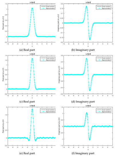
Figure 1. Example 1. Numerical results under the posteriori fractional Tikhonov method. (a,b) are real part and imaginary part at y = 0.2, respectively, where $\mu =1\times {10}^{-3}$; (c,d) are real part and imaginary part at y = 0.5, respectively, where $\mu =1\times {10}^{-3}$; (e,f) are real part and imaginary part at y = 0.8, respectively, where $\mu =1\times {10}^{-3}$.

Table 1 shows the different error results for different y in Example 1. We fix $\tau =50$, $\delta =0.01$ and compare the numerical results when $\gamma =2/3$ and $\gamma =1$. From Table 1, we can see that the numerical result of $\gamma =2/3$ is better than the numerical result of $\gamma =1$.

Table 1. Numerical results of Example 1 for different y and $\gamma$.

y		0.2	0.5	0.8
$\gamma =2/3$	$RMS{E}_{Re}$	0.0725	0.1009	0.2769
	$RMS{E}_{Im}$	0.0168	0.0732	0.2684
$\gamma =1$	$RMS{E}_{Re}$	0.0857	0.2866	0.7765
	$RMS{E}_{Im}$	0.0238	0.2774	0.7227

Example 2.

The function h is given by:

$$\begin{array}{c}\hfill h(z)=\left\{\begin{array}{cc}\sqrt{25-z^2}=\sqrt{25-{(x+iy)}^2},\hfill & \left|x\right|<5,\hfill \\ 0,\hfill & \left|x\right|\ge 5.\hfill \end{array}\right.\end{array}$$

It is a piecewise analytic function, and $\sqrt{25-{(x+iy)}^2}$ has a single-valued determination in the complex plane minus the set $x:\left|x\right|\ge 5$.

Figure 2 shows the numerical results of the a posteriori parameter selection of Example 2. $\mu$ is selected by the discrepancy principle (11), where $\tau =1.1,\delta =0.01$. Figure 2a–f show the comparison of the exact solution and the approximate solution at $y=0.2$$y=0.5$ and $y=0.8$.

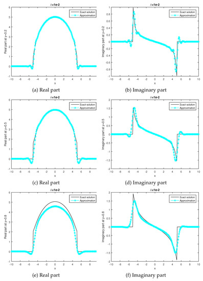
Figure 2. Example 2. Numerical results under the posteriori fractional Tikhonov method. (a,b) are the real part and imaginary part at y = 0.2, respectively, where $\mu =1\times {10}^{-4}$; (c,d) are the real part and imaginary part at y = 0.5, respectively, where $\mu =0.01$; (e,f) are the real part and imaginary part at y = 0.8, respectively, where $\mu =0.1$.

Table 2 shows the different error results for different y in Example 2. We fix $\tau =1.1$, $\delta =0.01$ and use $\gamma =2/3$ and $\gamma =1$ for comparison. According to the data in Table 1 and Table 2, it is not difficult to see that the fractional Tikhonov method is better than the classical Tikhonov method.

Table 2. Numerical results of Example 2 for different y and $\gamma$.

y		0.2	0.5	0.8
$\gamma =2/3$	$RMS{E}_{Re}$	1.2201	3.2006	5.1905
	$RMS{E}_{Im}$	1.2208	2.0412	2.8628
$\gamma =1$	$RMS{E}_{Re}$	1.6075	5.6605	6.5887
	$RMS{E}_{Im}$	1.7714	3.5022	3.7275

4. Conclusions

In this article, a fractional Tikhonov regularization method for analytic continuation problem is given, and we overcome its ill-posedness and obtained a regularized solution. Furthermore, we proved the error estimates for the fractional regularization methods under the the Morozov’s parameter choice rule. The numerical experiment shows that the proposed method works effectively. It is worth pointing out that the method we provide not only includes the classical Tikhonov regularization method, but the numerical results obtained are also more accurate and stable. Future research will extend the analytical continuation problem of one-dimensional cases to two-dimensional cases or even higher-dimensional cases. At the same time, other regularization methods will be tried to solve such inverse problems in order to obtain more accurate convergence results.

References

- Franklin, J. Analytic contiunation by the fast Fourier transform. SIAM. Sci. Stat. Comput. 1990, 11, 112–122. [Google Scholar] [CrossRef][Green Version]
- Ramm, A.G. The ground-penetrating radar problem. J. Inverse Ill-Posed Problem. 2000, 8, 23–30. [Google Scholar] [CrossRef][Green Version]
- Stefanescu, I.S. On the stable analytic continuation with a condition of uniform boundedness. J. Math. Phys. 1986, 27, 2657–2686. [Google Scholar] [CrossRef]
- Natterer, F. Image reconstruction in quantitative susceptibility mappling. SIAM J. Imaging Sci. 2016, 9, 1127–1131. [Google Scholar] [CrossRef]
- Airapetyan, R.G.; Ramm, A.G. Numerical inversion of the Laplace transform from the real axis. J. Math. Anal. Appl. 2000, 248, 572–587. [Google Scholar] [CrossRef]
- Epstein, C.L. Philadelphia. In Introduction to the Mathematics of Medical Imaging; SIAM: Philadelphia, PA, USA, 2008. [Google Scholar]
- Miller, K.; Viano, G.A. On the necessity of nearlybestpossible methods for analytic continuation of scattering data. J. Math. Phys. 1973, 14, 1037–1048. [Google Scholar] [CrossRef]
- Fu, C.L.; Deng, Z.L.; Feng, X.L.; Dou, F.F. A modified Tikhonov regularization for stable analytic continuation. SIAM J. Numer. Anal. 2009, 47, 2982–3000. [Google Scholar] [CrossRef]
- Engl, H.W.; Hanke, M.; Neubauer, A. Regularization of Inverse Problem; Kluwer Academic: Boston, MA, USA, 1996. [Google Scholar]
- Hao, D.N.; Shali, H. Stable analytic continuation by mollification and the fast Fourier transform. In Method of Complex and Clifford Analysis; ICAM: Hanoi, Vietnam, 2004; pp. 143–152. [Google Scholar]
- Deng, Z.L.; Fu, C.L.; Feng, X.L.; Zhang, Y.X. A mollification regularization method for stable analytic continuation. Math. Comput. Simul. 2011, 81, 1593–1608. [Google Scholar] [CrossRef]
- Fu, C.L.; Dou, F.F.; Feng, X.L.; Qian, Z. A simple regularization method for stable analytic continuation. Inverse Probl. 2008, 24, 065003. [Google Scholar] [CrossRef]
- Zhang, Y.X.; Fu, C.L.; Yan, L. Approximate inverse method for stable analytic continuation in a strip domain. J. Comput. Appl. Math. 2011, 235, 2979–2992. [Google Scholar] [CrossRef][Green Version]
- Cheng, H.; Fu, C.L.; Feng, X.L. An optimal filtering method for stable analytic continuation. J. Comput. Appl. Math. 2012, 236, 2582–2589. [Google Scholar] [CrossRef]
- Feng, X.L.; Ning, W.T. A wavelet regularization method for solving numerical analytic continuation. Int. J. Comput. Math. 2015, 92, 1025–1038. [Google Scholar] [CrossRef]
- Xiong, X.T.; Zhu, L.Q.; Li, M. Regularization methods for a problem of analytic continuation. Math. Comput. Simulat. 2011, 82, 332–345. [Google Scholar] [CrossRef]
- Cheng, H.; Fu, C.L.; Zhang, Y.X. An iteration method for stable analytic continuation. Appl. Math. Comput. 2014, 233, 203–213. [Google Scholar] [CrossRef]
- Xiong, X.T.; Cheng, Q. A modified Lavrentiev iterative regularization method for analytic continuation. J. Comput. Appl. Math. 2018, 327, 127–140. [Google Scholar] [CrossRef]
- Yang, F.; Wang, Q.C.; Li, X.X. A fractional Landweber iterative regularization method for stable analytic continuation. AIMS Math. 2021, 6, 404–419. [Google Scholar] [CrossRef]
- Klann, E.; Maass, P.; Ramlau, R. Two-step regularization methods for linear inverse problems. J. Inverse Ill-Posed Probl. 2006, 14, 583–609. [Google Scholar] [CrossRef]
- Tikhonov, A.N.; Goncharsky, A.V.; Stepanov, V.V.; Yagola, A.G. Numerical Methods for the Solution of Ill-Posed Problems; Kluwer Academic Publishers: Dordrecht, The Netherlands, 1995. [Google Scholar]
- Klann, E.; Ramlau, R. Regularization by fractional filter methods and data smoothing. Inverse Probl. 2008, 24, 045005. [Google Scholar] [CrossRef]
- Hochstenbach, M.E.; Reichel, L. Fractional Tikhonov regularization for linear discrete ill-posed problems. BIT Numer. Math. 2011, 51, 197–215. [Google Scholar] [CrossRef]
- Gerth, D.; Klann, E.; Ramlau, R.; Reichel, L. On fractional Tikhonov regularization. J. Inverse Ill-Posed Probl. 2015, 23, 611–625. [Google Scholar] [CrossRef]
- Morigi, S.; Reichel, L.; Sgallari, F. Fractional Tikhonov regularization with a nonlinear penalty term. J. Comput. Appl. Math. 2017, 324, 142–154. [Google Scholar] [CrossRef]
- Bianchi, D.; Buccini, A.; Donatelli, M.; Serra-Capizzano, S. Iterated fractional Tikhonov regularization. Inverse Probl. 2015, 31, 055005. [Google Scholar] [CrossRef]
- Bianchi, D.; Donatelli, M. On generalized iterated Tikhonov regularization with operator-dependent seminorms. Electron. Trans. Numer. Anal. 2017, 47, 73–99. [Google Scholar] [CrossRef]
- Xiong, X.T.; Xue, X.M.; Qian, Z. A modified iterative regularization method for ill-posed problems. Appl. Numer. Math. 2017, 122, 108–128. [Google Scholar] [CrossRef]
- Li, M.; Xiong, X.T. On a fractional backward heat conduction problem: Application to deblurring. Comput. Math. Appl. 2012, 64, 2594–2602. [Google Scholar] [CrossRef]
- Qian, Z. A new generalized Tikhonov method based on filtering idea for stable analytic continuation. Inverse. Probl. Sci. Eng. 2018, 26, 362–375. [Google Scholar] [CrossRef]
- Morozov, V.A. Regularization of incorrectly posed problems and the choice of regularization parameter. USSR Comput. Math. Math. Phys. 1966, 6, 242–251. [Google Scholar] [CrossRef]
- Xiong, X.T. A regularization method for a Cauchy problem of the Helmholtz equation. J. Comput. Appl. Math. 2010, 233, 1723–1732. [Google Scholar] [CrossRef][Green Version]
Publisher’s Note: MDPI stays neutral with regard to jurisdictional claims in published maps and institutional affiliations. |
© 2021 by the authors. Licensee MDPI, Basel, Switzerland. This article is an open access article distributed under the terms and conditions of the Creative Commons Attribution (CC BY) license (https://creativecommons.org/licenses/by/4.0/).