Abstract
In this paper, we present a new asymptotically normal test for out-of-sample evaluation in nested models. Our approach is a simple modification of a traditional encompassing test that is commonly known as Clark and West test (CW). The key point of our strategy is to introduce an independent random variable that prevents the traditional CW test from becoming degenerate under the null hypothesis of equal predictive ability. Using the approach developed by West (1996), we show that in our test, the impact of parameter estimation uncertainty vanishes asymptotically. Using a variety of Monte Carlo simulations in iterated multi-step-ahead forecasts, we evaluated our test and CW in terms of size and power. These simulations reveal that our approach is reasonably well-sized, even at long horizons when CW may present severe size distortions. In terms of power, results were mixed but CW has an edge over our approach. Finally, we illustrate the use of our test with an empirical application in the context of the commodity currencies literature.
1. Introduction
Forecasting is one of the most important and widely studied areas in time series econometrics. While there are many challenges related to financial forecasting, forecast evaluation is a key topic in the field. One of the challenges faced by the forecasting literature is the development of adequate tests to conduct inference about predictive ability. In what follows, we review some advances in this area and address some of the remaining challenges.
“Mighty oaks from little acorns grow”. This is probably the best way to describe the forecast evaluation literature since the mid-1990s. The seminal works of Diebold and Mariano (1995) [1] and West (1996) [2] (DMW) have flourished in many directions, attracting the attention of both scholars and practitioners in the quest for proper evaluation techniques. See West (2006) [3], Clark and McCracken (2013) [4], and Giacomini and Rossi (2013) [5] for great reviews on forecasting evaluation.
Considering forecasts as primitives, Diebold and Mariano (1995) [1] showed that under mild conditions on forecast errors and loss functions, standard time-series versions of the central limit theorem apply, ensuring asymptotic normality for tests evaluating predictive performance. West (1996) [2] considered the case in which forecasts are constructed with estimated econometric models. This is a critical difference with respect to Diebold and Mariano (1995) [1], since forecasts are now polluted by estimation error.
Building on this insight, West (1996) [2] developed a theory for testing population-level predictive ability (i.e., using estimated models to learn something about the true models). Two fundamental issues arise from West’s contribution: Firstly, in some specific cases, parameter uncertainty is “asymptotically irrelevant”, hence, it is possible to proceed as proposed by Diebold and Mariano (1995) [1]. Secondly, although West’s theory is quite general, it requires a full rank condition over the long-run variance of the objective function when parameters are set at their true values. A leading case in which this assumption is violated is in standard comparisons of mean squared prediction errors (MSPE) in nested environments.
As pointed out by West (2006) [3]: “A rule of thumb is: if the rank of the data becomes degenerate when regression parameters are set at their population values, then a rank condition assumed in the previous sections likely is violated. When only two models are being compared, “degenerate” means identically zero” West (2006) [3], page 117. Clearly, in the context of two nested models, the null hypothesis of equal MSPE means that both models are exactly the same, which generates the violation of the rank condition in West (1996) [2].
Forecast evaluations in nested models are extremely relevant in economics and finance for at least two reasons. Firstly, it is a standard in financial econometrics to compare the predictive accuracy of a given model A with a simple benchmark that usually is generated from a model B, which is nested in A (e.g., the ‘no change forecast’). Some of the most influential empirical works, like Welch and Goyal (2008) [6] and Meese and Rogoff (1983, 1988) [7,8], have shown that outperforming naïve models is an extremely difficult task. Secondly, comparisons within the context of nested models provide an easy and intuitive way to evaluate and identify the predictive content of a given variable Xt: suppose the only difference between two competing models is that one of them uses the predictor Xt, while the other one does not. If the former outperforms the latter, then Xt has relevant information to predict the target variable.
Due to its relevance, many efforts have been undertaken to deal with this issue. Some key contributions are those of Clark and McCracken (2001, 2005) [9,10] and McCracken (2007) [11], who used a different approach that allows for comparisons at the population level between nested models. Although, in general, the derived asymptotic distributions are not standard, for some specific cases (e.g., no autocorrelation, conditional homoskedasticity of forecast errors, and one-step-ahead forecasts), the limiting distributions of the relevant statistics are free of nuisance parameters, and their critical values are provided in Clark and McCracken (2001) [9].
While the contributions of many authors in the last 25 years have been important, our reading of the state of the art in forecast evaluation coincides with the view of Diebold (2015) [12]: “[…] one must carefully tiptoe across a minefield of assumptions depending on the situation. Such assumptions include but are not limited to: (1) Nesting structure and nuisance parameters. Are the models nested, non-nested, or partially overlapping? (2) Functional form. Are the models linear or nonlinear? (3) Model disturbance properties. Are the disturbances Gaussian? Martingale differences? Something else? (4) Estimation sample. Is the pseudo-in-sample estimation period fixed? Recursively expanding? Something else? (5) Estimation method. Are the models estimated by OLS? MLE? GMM? Something else? And crucially: Does the loss function embedded in the estimation method match the loss function used for pseudo-out-of-sample forecast accuracy comparisons? (6) Asymptotics. What asymptotics are invoked?” Diebold (2015) [12], pages 3–4. Notably, the relevant limiting distribution generally depends on some of these assumptions.
In this context, there is a demand for straightforward tests that simplify the discussion in nested model comparisons. Of course, there have been some attempts in the literature. For instance, one of the most used approaches in this direction is the test outlined in Clark and West (2007) [13]. The authors showed, via simulations, that standard normal critical values tend to work well with their test, even though, Clark and McCracken (2001) [9] demonstrated that this statistic has a non-standard distribution. Moreover, when the null model is a martingale difference and parameters are estimated with rolling regressions, Clark and West (2006) [14] showed that their test is indeed asymptotically normal. Despite this and other particular cases, as stated in the conclusions of West (2006) [3] review: “One of the highest priorities for future work is the development of asymptotically normal or otherwise nuisance parameter-free tests for equal MSPE or mean absolute error in a pair of nested models. At present only special case results are available”. West (2006) [3], page 131. Our paper addresses this issue.
Our WCW test can be viewed as a simple modification of the CW test. As noticed by West (1996) [2], in the context of nested models, the CW core statistic becomes degenerate under the null hypothesis of equal predictive ability. Our suggestion is to introduce an independent random variable with a “small” variance in the core statistic. This random variable prevents our test from becoming degenerate under the null hypothesis, keeps the asymptotic distribution centered around zero, and eliminates the autocorrelation structure of the core statistic at the population level. While West’s (1996) [2] asymptotic theory does not apply for CW (as it does not meet the full rank condition), it does apply for our test (as the variance of our test statistic remains positive under the null hypothesis). In this sense, our approach not only prevents our test from becoming degenerate, but also ensures asymptotic normality relying on West’s (1996) [2] results. In a nutshell, there are two key differences between CW and our test. Firstly, our test is asymptotically normal, while CW is not. Secondly, our simulations reveal that WCW is better sized than CW, especially at long forecasting horizons.
We have also demonstrated that “asymptotic irrelevance” applies; hence the effects of parameter uncertainty can be ignored. As asymptotic normality and “asymptotic irrelevance” apply, our test is extremely user friendly and easy to implement. Finally, one possible concern about our test is that it depends on one realization of one independent random variable. To partially overcome this issue, we have also provided a smoothed version of our test that relies on multiple realizations of this random variable.
Most of the asymptotic theory for the CW test and other statistics developed in Clark and McCracken (2001, 2005) [9,10] and McCracken (2007) [11] focused almost exclusively on direct multi-step-ahead forecasts. However, with some exceptions (e.g., Clark and McCracken (2013) [15] and Pincheira and West (2016) [16]), iterated multi-step-ahead forecasts have received much less attention. In part for this reason, we evaluated the performance of our test (relative to CW), focusing on iterated multi-step-ahead forecasts. Our simulations reveal that our approach is reasonably well-sized, even at long horizons when CW may present severe size distortions. In terms of power, results have been rather mixed, although CW has frequently exhibited some more power. All in all, our simulations reveal that asymptotic normality and size corrections come with a cost: the introduction of a random variable erodes some of the power of WCW. Nevertheless, we also show that the power of our test improves with a smaller variance of our random variable and with an average of multiple realizations of our test.
Finally, based on the commodity currencies literature, we provide an empirical illustration of our test. Following Chen, Rossi, and Rogoff (2010, 2011) [17,18]; Pincheira and Hardy (2018, 2019, 2021) [19,20,21]; and Pincheira and Jarsun (2020) [22], we evaluated the performance of the exchange rates of three major commodity exporters (Australia, Chile, and South Africa) when predicting commodity prices. Consistent with previous literature, we found evidence of predictability for some of the commodities considered in this exercise. Particularly strong results were found when predicting the London Metal Exchange Index, aluminum and tin. Fairly interesting results were also found for oil and the S&P GSCI. The South African rand and the Australian dollar have a strong ability to predict these two series. We compared our results using both CW and WCW. At short horizons, both tests led to similar results. The main differences appeared at long horizons, where CW tended to reject the null hypothesis of no predictability more frequently. From the lessons learned from our simulations, we can think of two possible explanations for these differences: Firstly, they might be the result of CW displaying more power than WCW. Secondly, they might be the result of CW displaying a higher false discovery rate relative to WCW. Let us recall that CW may be severely oversized at long horizons, while WCW is better sized. These conflicting results between CW and WCW might act as a warning of a potential false discovery of predictability. As a consequence, our test brings good news to careful researchers that seriously wish to avoid spurious findings.
The rest of this paper is organized as follows. Section 2 establishes the econometric setup and forecast evaluation framework, and presents the WCW test. Section 3 addresses the asymptotic distribution of the WCW, showing that “asymptotic irrelevance” applies. Section 4 describes our DGPs and simulation setups. Section 5 discusses the simulation results. Section 6 provides an empirical illustration. Finally, Section 7 concludes.
2. Econometric Setup
Consider the following two competing nested models for a target scalar variable .
where and are both zero mean martingale difference processes, meaning that for and stands for the sigma field generated by current and past values of and . We will assume that and have finite and positive fourth moments.
When the econometrician wants to test the null using an out-of-sample approach in this econometric context, Clark and McCracken (2001) [9] derived the asymptotic distribution of a traditional encompassing statistic used, for instance, by Harvey, Leybourne, and Newbold (1998) [23] (other examples of encompassing tests include Chong and Hendry (1986) [24] and Clements and Hendry (1993) [25], to name a few). In essence, the ENC-t statistic proposed by Clark and McCracken (2001) [9] studies the covariance between and . Accordingly, this test statistic takes the form:
where is the usual variance estimator for and P is the number of out-of-sample forecasts under evaluation (as pointed out by Clark and McCracken (2001) [9], the HLN test is usually computed with regression-based methods. For this reason, we use rather than ). See Appendix A.1 for two intuitive interpretations of the ENC-t test.
The null hypothesis of interest is that . This implies that . This null hypothesis is also equivalent to equality in MSPE.
Even though West (1996) [2] showed that the ENC-t is asymptotically normal for non-nested models, this is not the case in nested environments. Note that one of the main assumptions in West’s (1996) [2] theory is that the population counterpart of is strictly positive. This assumption is clearly violated when models are nested. To see this, recall that under the null of equal predictive ability, and for all t. In other words, the population prediction errors from both models are identical under the null and, therefore, is exactly zero. Consequently, . More precisely, notice that under the null:
It follows that the rank condition in West (1996) [2] cannot be met as .
The main aim of our paper was to modify this ENC-t test to make it asymptotically normal under the null. Our strategy required the introduction of a sequence of independent random variables with variance and expected value equal to 1. It is critical to notice that is not only i.i.d, but also independent from and .
With this sequence in mind, we define our “Wild Clark and West” (WCW-t) statistic as
where is a consistent estimate of the long-run variance of (e.g., Newey and West (1987, 1994) [26,27] or Andrews (1991) [28]).
In this case, under the null we have , therefore:
Besides, we have that under the null
The last result follows from the fact that . Notice that this transformation is important: under the null hypothesis, even if is identically zero for all t, the inclusion of prevents the core statistic from becoming degenerate, preserving a positive variance (it is also possible to show that the term has no autocorrelation under the null).
Additionally, under the alternative:
Therefore:
Consequently, our test is one-sided.
Finally, there are two possible concerns with the implementation of our WCW-t statistic. The first one is about the choice of . Even though this decision is arbitrary, we give the following recommendation: should be “small”; the idea of our test is to recover asymptotic normality under the null hypothesis, something that could be achieved for any value of . However, if is “too big”, it may simply erode the predictive content under the alternative hypothesis, deteriorating the power of our test. Notice that a “small” variance for some DGPs could be a “big” one for others, for this reason, we propose to take as a small percentage of the sample counterpart of . As we discuss later in Section 4, we considered three different standard deviations with reasonable size and power results: (1 percent, 2 percent, and 4 percent of the standard deviation of ). We emphasize that is the sample variance of the estimated forecast errors. Obviously, our test tends to be better sized as grows, at the cost of some power.
Secondly, notice that our test depends on realization of the sequence . One reasonable concern is that this randomness could strongly affect our WCW-t statistic (even for “small” values of the parameter). In other words, we would like to avoid significant changes in our statistic generated by the randomness of . Additionally, as we report in Section 4, our simulations suggest that using just one realization of the sequence sometimes may significantly reduce the power of our test relative to CW. To tackle both issues, we propose to smooth the randomness of our approach by considering different WCW-t statistics constructed with different and independent sequences of . Our proposed test is the simple average of these standard normal WCW-t statistics, adjusted by the correct variance of the average as follows:
where is the k-th realization of our statistic and is the sample correlation between the i-th and j-th realization of the WCW-t statistics. Interestingly, as we discuss in Section 4, when using , the size of our test is usually stable, but it significantly improves the power of our test.
3. Asymptotic Distribution
Since most of our results rely on West (1996) [2], here we introduce some of his results and notation. For clarity of exposition, we focus on one-step-ahead forecasts. The generalization to multi-step-ahead forecasts is cumbersome in notation but straightforward.
Let be our loss function. We use “*” to emphasize that depends on the true population parameters, hence , where . Additionally, let be the sample counterpart of . Notice that rely on estimates of , and as a consequence, is polluted by estimation error. Moreover, notice the subindex in : the out-of-sample forecast errors ( and ) depend on the estimates constructed with the relevant information available up to time t. These estimates can be constructed using either rolling, recursive, or fixed windows. See West (1996, 2006) [2,3] and Clark and McCracken (2013) [4] for more details about out-of-sample evaluations.
Let be the expected value of our loss function. As considered in Diebold and Mariano (1995) [1], if predictions do not depend on estimated parameters, then under weak conditions, we can apply the central limit theorem:
where stands for the long-run variance of the scalar . However, one key technical contribution of West (1996) [2] was the observation that when forecasts are constructed with estimated rather than true, unknown, population parameters, some terms in expression (2) must be adjusted. We remark here that we observe rather than . To see how parameter uncertainty may play an important role, under assumptions Appendix A.1, Appendix A.2, Appendix A.3 and Appendix A.4 in the Appendix A, West (1996) [2] showed that a second-order expansion of around yields
where , R denotes the length of the initial estimation window, and T is the total sample size (T = R + P), while will be defined shortly.
Recall that in our case, under the null hypothesis, , hence expression (3) is equivalent to
Note that according to West (2006) [3], p. 112, and in line with Assumption 2 in West (1996) [2], pp. 1070–1071, the estimator of the regression parameters satisfies
where is ; is with (a) as a matrix of rank k; (b) = if the estimation method is recursive, = if it is rolling, or = if it is fixed. is a orthogonality condition that is satisfied. Notice that ; (c) .
As explained in West (2006) [3]: “Here, can be considered as the score if the estimation method is ML, or the GMM orthogonality condition if GMM is the estimator. The matrix is the inverse of the Hessian if the estimation method is ML or a linear combination of orthogonality conditions when using GMM, with large sample counterparts .” West (2006) [3], p. 112.
Notice that Equation (3) clearly illustrates that can be decomposed into two parts. The first term of the RHS is the population counterpart, whereas the second term captures the sequence of estimates of (in other words, terms arising because of parameter uncertainty). Then, as , we can apply the expansion in West (1996) [2] as long as assumptions of Appendix A.1, Appendix A.2, Appendix A.3 and Appendix A.4 hold. The key point is that a proper estimation of the variance in Equation (3) must account for: (i) the variance of the first term of the RHS (, i.e., the variance when there is no uncertainty about the population parameters), (ii) the variance of the second term of the RHS, associated with parameter uncertainty, and iii) the covariance between both terms. Notice, however, that parameter uncertainty may be “asymptotically irrelevant” (hence (ii) and (iii) may be ignored) in the following cases: (1) as , (2) a fortunate cancellation between (ii) and (iii), or (3) .
In our case:
where
Note that under the null, and recall that , therefore
With a similar argument, it is easy to show that
Finally,
This result follows from the fact that we define as a martingale difference with respect to and .
Hence, in our case “asymptotic irrelevance” applies as and Equation (3) reduces simply to
In other words, we could simply replace true errors by estimated out-of-sample errors and forget about parameter uncertainty, at least asymptotically.
4. Monte Carlo Simulations
In order to capture features from different economic/financial time series and different modeling situations that might induce a different behavior in the tests under evaluation, we considered three DGPs. The first DGP (DGP1) relates to the Meese–Rogoff puzzle and matches exchange rate data (Meese and Rogoff (1983,1988) [7,8] found that, in terms of predictive accuracy, many exchange rate models perform poorly against a simple random walk). In this DGP, under the null hypothesis, the target variable is simply white noise. In this sense, DGP1 mimics the low persistence of high frequency exchange rate returns. While in the null model, there are no parameters to estimate, under the alternative model there is only one parameter that requires estimation. Our second DGP matches quarterly GDP growth in the US. In this DGP, under the null hypothesis, the target variable follows an AR(1) process with two parameters requiring estimation. In addition, the alternative model has four extra parameters to estimate. Differing from DGP1, in DGP 2, parameter uncertainty may play an important role in the behavior of the tests under evaluation. DGP1 and DGP2 model stationary variables with low persistence, such as exchange rate returns and quarterly GDP growth. To explore the behavior of our tests with a series displaying more persistence, we considered DGP3. This DGP is characterized by a VAR(1) model in which both the predictor and the predictand are stationary variables that display relatively high levels of persistence. In a nutshell, there are three key differences in our DGPs: persistence of the variables, the number of parameters in the null model, and the number of excess parameters in the alternative model (according to Clark and McCracken (2001) [9], the asymptotic distribution of the ENC-t, under the null hypothesis, depends on the excess of parameters in the alternative model—as a consequence, the number of parameters in both the null and alternative models are key features of these DGPs).
To save space, we only report here results for recursive windows, although in general terms, results with rolling windows were similar and they are available upon request. For large sample exercises, we considered an initial estimation window of R = 450 and a prediction window of P = 450 (T = 900), while for small sample exercises, we considered R = 90 and P = 90 (T = 180). For each DGP, we ran 2000 independent replications. We evaluated the CW test and our test, computing iterated multi-step-ahead forecasts at several forecasting horizons from h = 1 up to h = 30. As discussed at the end of Section 2, we computed our test using K = 1 and K = 2 realizations of our WCW-t statistic. Additionally, for each simulation, we considered three different standard deviations of : (1 percent, 2 percent, and 4 percent of the standard deviation of ). We emphasize that is the sample variance of the out-of-sample forecast errors and it was calculated for each simulation.
Finally, we evaluated the usefulness of our approach using the iterated multistep ahead method for the three DGPs under evaluation (notice that the iterated method uses an auxiliary equation for the construction of the multistep ahead forecasts—here, we stretched the argument of “asymptotic irrelevance” and we assumed that parameter uncertainty on the auxiliary equation plays no role). We report our results comparing the CW and the WCW-t test using one-sided standard normal critical values at the 10% and 5% significance level (a summary of the results considering a 5% significance level can be found in the Appendix section). For simplicity, in each simulation we considered only homoscedastic, i.i.d, normally distributed shocks.
DGP 1
Our first DGP assumes a white noise for the null model. We considered a case like this given its relevance in finance and macroeconomics. Our setup is very similar to simulation experiments in Pincheira and West (2006) [16], Stambaugh (1999) [29], Nelson and Kim (1993) [30], and Mankiw and Shapiro (1986) [31].
Null model:
Alternative model:
We set our parameters as follows:
| under | under | |||||
| 1.19 | −0.25 | (1.75)2 | (0.075)2 | 0 | 0 | −2 |
The null hypothesis posits that follows a no-change martingale difference. Additionally, the alternative forecast for multi-step-ahead horizons was constructed iteratively through an AR(p) on . This is the same parametrization considered in Pincheira and West (2016) [16], and it is based on a monthly exchange rate application in Clark and West (2006) [14]. Therefore, represents the monthly return of a U.S dollar bilateral exchange rate and is the corresponding interest rate differential.
DGP 2
Our second DGP is mainly inspired by macroeconomic data, and it was also considered in Pincheira and West (2016) [16] and Clark and West (2007) [13]. This DGP is based on models exploring the relationship between U.S GDP growth and the Federal Reserve Bank of Chicago’s factor index of economic activity.
Null model:
Alternative model:
We set our parameters as follows:
| under | under | under | under |
| 0 | 0 | 0 | 0 |
| under | under | under | under |
| 3.363 | −0.633 | −0.377 | −0.529 |
| 0.261 | 10.505 | 0.366 | 0.528 |
DGP 3
Our last DGP follows Busetti and Marcucci (2013) [32] and considers a very simple VAR(1) process:
Null model:
Alternative model:
We set our parameters as follows:
| c under | c under | |||||
| 0.8 | 0.8 | 1 | 1 | 0 | 0 | 0.5 |
5. Simulation Results
This section reports exclusively results for a nominal size of 10%. To save space, we considered only results with a recursive scheme. Results with rolling windows were similar, and they are available upon request. Results of the recursive method are more interesting to us for the following reason: For DGP1, Clark and West (2006) [14] showed that the CW statistic with rolling windows is indeed asymptotically normal. In this regard, the recursive method may be more interesting to discuss due to the expected departure from normality in the CW test. For each simulation, we considered i.i.d normally distributed with mean one and variance . Table 1, Table 2, Table 3, Table 4, Table 5 and Table 6 show results on size considering different choices for and K, as suggested at the end of Section 2. The last row of each table reports the average size for each test across the 30 forecasting horizons. Table 7, Table 8, Table 9, Table 10, Table 11 and Table 12 are akin to Table 1, Table 2, Table 3, Table 4, Table 5 and Table 6, but they report results on power. Similarly to Table 1, Table 2, Table 3, Table 4, Table 5 and Table 6, the last row of each table reports the average power for each test across the 30 forecasting horizons. Our analysis with a nominal size of 5% carried the same message. A summary of these results can be found in the Appendix.

Table 1.
Empirical size comparisons between CW and WCW tests with nominal size of 10%, considering DGP1 and a large sample.
Table 2.
Empirical size comparisons between CW and WCW tests with nominal size of 10%, considering DGP1 and a small sample.
Table 3.
Empirical size comparisons between CW and WCW tests with nominal size of 10%, considering DGP2 and a large sample.
Table 4.
Empirical size comparisons between CW and WCW tests with nominal size of 10%, considering DGP2 and a small sample.
Table 5.
Empirical size comparisons between CW and WCW tests with nominal size of 10%, considering DGP3 and a large sample.
Table 6.
Empirical size comparisons between CW and WCW tests with nominal size of 10%, considering DGP3 and a small sample.
Table 7.
Power comparisons between CW and WCW tests with nominal size of 10%, considering DGP1 and a large sample.
Table 8.
Power comparisons between CW and WCW tests with nominal size of 10%, considering DGP1 and a small sample.
Table 9.
Power comparisons between CW and WCW tests with nominal size of 10%, considering DGP2 and a large sample.
Table 10.
Power comparisons between CW and WCW tests with nominal size of 10%, considering DGP2 and a small sample.
Table 11.
Power comparisons between CW and WCW tests with nominal size of 10%, considering DGP3 and a large sample.
Table 12.
Power comparisons between CW and WCW tests with nominal size of 10%, considering DGP3 and a small sample.
5.1. Simulation Results: Size
Table 1 reports results for the case of a martingale sequence (i.e., DGP1) using large samples (P = R = 450 and T = 900). From the second column of Table 1, we observed that the CW test was modestly undersized. The empirical size of nominal 10% tests ranged from 6% to 8%, with an average size across the 30 forecasting horizons of 6%. These results are not surprising. For instance, for the case of a martingale sequence, Clark and West (2006) [14] commented that: “our statistic is slightly undersized, with actual sizes ranging from 6.3% […] to 8.5%” Clark and West (2006) [14], pp. 172–173. Moreover, Pincheira and West (2016) [16], using iterated multi-step ahead forecasts, found very similar results.
Our test seemed to behave reasonably well. Across the nine different exercises presented in Table 1, the empirical size of our WCW test ranged from 7% to 11%. Moreover, the last row indicates that the average size of our exercises ranged from 0.08 () to 0.10 (e.g., all exercises considering ). Notably, our results using “the highest variance”, , ranged from 9% to 11%, with an average size of 10% in the two cases. As we discuss in the following section, in some cases, this outstanding result comes at the cost of some reduction in power.
Table 2 is akin to Table 1, but considering simulations with small samples (P = R = 90 and T = 180). While the overall message was very similar, the CW test behaved remarkably well, with an empirical size ranging from 8% to 10% and an average size of 9%. Additionally, our test also showed good size behavior, but with mild distortions in some experiments. Despite these cases, in 6 out of 9 exercises, our test displayed an average size of 10% across different forecast horizons. The main message of Table 1 and Table 2 is that our test behaves reasonably well, although there were no great improvements (nor losses) compared to CW.
Table 3 reports our results for DGP2 using large samples (P = R = 450 and T = 900). In this case, the empirical size of the CW test ranged from 8% to 16%, with an average size of 13%. Notably, the CW test was undersized at “short” forecasting horizons () and oversized at long forecasting horizons (). This is consistent with the results reported in Pincheira and West (2016) [16] for the same DGP using a rolling scheme: “[…] the CW test has a size ranging from 7% to 13%. It tends to be undersized at shorter horizons (), oversized at longer horizons ().” Pincheira and West (2016) [16], p. 313.
In contrast, our test tended to be considerably better sized. Across all exercises, the empirical size of the WCW ranged from 8% to 12%. Moreover, the average size for each one of our tests was in the range of 10% to 11%. In sharp contrast with CW, our test had a “stable” size and did not become increasingly oversized with the forecasting horizon. In particular, for h = 30, the empirical size of our test across all exercises was exactly 10%, while CW had an empirical size of 15%. In this sense, our test offers better protection to the null hypothesis at long forecasting horizons.
Table 4 is akin to Table 3, but considering a smaller sample. The overall message is similar, however, both CW and our test became oversized. Despite these size distortions in both tests, we emphasize that our test performed comparatively better relative to CW in almost every exercise. For instance, using a standard deviation of or , our test was reasonably well-sized across all exercises. The worst results were found for ; however, our worst exercise, with K = 2, was still better (or equally) sized compared to CW for all horizons. The intuition of presenting the worst results is, in fact, by construction; recall that for , our test coincided with CW, hence, as the variance of becomes smaller, it is reasonable to expect stronger similarities between CW and our test. In a nutshell, Table 3 and Table 4 indicate that our test is reasonably well sized, with some clear benefits compared to CW for long horizons (e.g., ), as CW becomes increasingly oversized.
Finally, Table 5 and Table 6 show our results for DGP3 using large samples (P = R = 450 and T = 900) and small samples (P = R = 90 and T = 180), respectively. The main message is very similar to that obtained from DGP2—CW was slightly undersized at short forecasting horizons (e.g., ) and increasingly oversized at longer horizons (). In contrast, our test either did not exhibit this pattern with the forecasting horizon or, when it did, it was milder. Notably, for long horizons (e.g., h = 30) our test was always better sized than CW. As in the previous DGP, our test worked very well using “the higher variance” and became increasingly oversized as the standard deviation approached zero. Importantly, using the two highest variances ( and ) our worst results were empirical sizes of 16%; in sharp contrast, the worst entries for CW were 20% and 22%.
All in all, Table 1, Table 2, Table 3, Table 4, Table 5 and Table 6 provide a similar message: on average, our test seemed to be better sized, specially at long forecasting horizons. The size of our test improved with a higher , but as we will see in the following section, sometimes this improvement comes at the cost of a mild reduction in power.
5.2. Simulation Results: Power
The intuition of our test is that we achieve normality by introducing a random variable that prevents the core statistic of the CW test from becoming degenerate under the null hypothesis. As reported in the previous section, our test tended to display a better size relative to CW, especially at long horizons. The presence of this random variable, however, may also have eroded some of the predictive content of model 2, and consequently, it may also erode the power of our test. As we will see in this section, CW has an edge over WCW in terms of power (this was somewhat expected since CW exhibits some important size distortions). Nevertheless, we noticed that the power of WCW improved with the number of realizations of (K) and with a smaller variance of (ϕ). Table 7 and Table 8 report power results for DGP1, considering large and small samples, respectively. Table 7 shows results that are, more or less, consistent with the previous intuition—the worst results were found for the highest standard deviation () and one sequence of realizations of (K = 1). In this sense, the good results in terms of size reported in the previous section came at the cost of a slight reduction in power. In this case, the average loss of power across the 30 forecasting horizons was about 6% (55% for CW and 49% for our “less powerful” exercise). Notice, however, that averaging two independent realizations of our test (e.g., K = 2) or reducing , rapidly enhanced the power of our test. Actually, with and a low variance of , the power of our test became very close to that of CW. The best results in terms of power were found for the smallest variance. This can be partially explained by the fact that the core statistic of our test became exactly the CW core statistic when the variance approached zero. Table 8 shows results mostly in the same line, although this time figures are much lower due to the small sample. Importantly, differences in terms of power were almost negligible between our approach and CW.
Table 9 and Table 10 report power results for DGP2, considering large and small samples, respectively. Contrary to DGP1, now, power reductions using our approach are important for some exercises. For instance, in Table 10, CW had 20% more rejections than our “less powerful” exercise. In this sense, asymptotic normality and good results for in terms of size, came along with an important reduction in power. As noticed before, the power of our test rapidly improved with K > 1 or with a smaller . For instance, in Table 10, for the case of , if we considered K = 2 instead of K = 1, the average power improved from 37% to 43%. Moreover, if we kept K = 2 and reduced to , differences in power compared to CW were small.
Finally, Table 11 and Table 12 report power results for DGP3, considering large and small samples, respectively. In most cases reductions in power were small (if any). For instance, our “less powerful exercise” in Table 11 had an average power only 3% below CW (although there were some important differences at long forecasting horizons, such as h = 30). However, as commented previously, the power of our test rapidly improved when considering ; in this case, differences in power were fairly small for all exercises. Notably, in some cases we found tiny (although consistent) improvements in power over CW; for instance, using the smallest standard deviation and K = 2, our test was “as powerful” as CW, and sometimes even slightly more powerful for longer horizons (e.g., h > 18).
All in all, our simulations reveal that asymptotic normality and size corrections come with a cost: The introduction of the random variable tended to erode some of the power of our test. In this sense, there was a tradeoff between size and power in the WCW test. Nevertheless, our results are consistent with the idea that the power improves with an average of K realizations of , and with a smaller variance of (). An interesting avenue for further research would be to explore different strategies to maximize this size/power tradeoff (e.g., an optimal criteria for K and ).
5.3. Simulation Results: Some Comments on Asymptotic Normality
Our simulation exercises show that CW has a pattern of becoming increasingly oversized with the forecasting horizon. At the same time, WCW tends to have a more “stable” size at long forecasting horizons. These results may, in part, be explained by a substantial departure from normality of CW as h grows. Using DGP2 with h = 12, 21, and 27, Figure 1, Figure 2 and Figure 3 support this intuition—while CW showed a strong departure from normality, our WCW seemed to behave reasonably well.
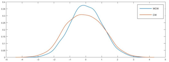
Figure 1.
Kernel densities of CW and WCW under the null hypothesis, DGP2, h = 12. Notes: For this exercise, we considered large samples (P = R = 450 and T = 900) and 4000 Monte Carlo simulations. We evaluated CW and our test computing iterated forecasts. In this case, we used WCW with K = 1 and .
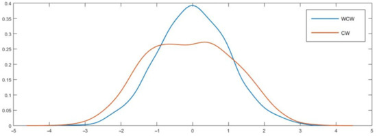
Figure 2.
Kernel densities of CW and WCW under the null hypothesis, DGP2, h = 21. Note: See notes in Figure 1.
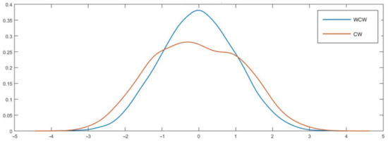
Figure 3.
Kernel densities of CW and WCW under the null hypothesis, DGP2, h = 27. Note: See notes in Figure 1.
Table 13 reports the means and the variances of CW and WCW after 4000 Monte Carlo simulations. As both statistics were standardized, we should expect means around zero, and variances around one (if asymptotic normality applies). Results in Table 13 are consistent with our previous findings—while the variance of CW was notably high for longer horizons (around 1.5 for h > 18), the variance of our test seemed to be stable with h, and tended to improve with a higher . In particular, for the last columns, the average variance of our test ranged from 1.01 to 1.02, and, moreover, none of the entries were higher than 1.05 nor lower than 0.98. In sharp contrast, the average variance of CW was 1.32, ranging from 1.07 through 1.51. All in all, these figures are consistent with the fact that WCW is asymptotically normal.
Table 13.
Means and variances of the CW and WCW statistics for DGP2 under the null hypothesis.
6. Empirical Illustration
Our empirical illustration was inspired by the commodity currencies literature. Relying on the present value model for exchange rate determination (Campbell and Shiller (1987) [33] and Engel and West (2005) [34]), Chen, Rogoff, and Rossi (2010, 2011) [17,18]; Pincheira and Hardy (2018, 2019, 2021) [19,20,21]; and many others showed that the exchange rates of some commodity-exporting countries have the ability to predict the prices of the commodities being exported and other closely related commodities as well.
Based on this evidence, we studied the predictive ability of three major commodity-producer’s economies frequently studied by this literature: Australia, Chile, and South Africa. To this end, we considered the following nine commodities/commodity indices: (1) WTI oil, (2) copper, (3) S&P GSCI: Goldman Sachs Commodity Price Index, (4) aluminum, (5) zinc, (6) LMEX: London Metal Exchange Index, (7) lead, (8) nickel, and (9) tin.
The source of our data was the Thomson Reuters Datastream, from which we downloaded the daily close price of each asset. Our series was converted to the monthly frequency by sampling from the last day of the month. The time period of our database went from September 1999 through June 2019 (the starting point of our sample period was determined by the date in which monetary authorities in Chile decided to pursue a pure flotation exchange rate regime).
Our econometric specifications were mainly inspired by Chen, Rogoff, and Rossi (2010) [17] and Pincheira and Hardy (2018, 2019, 2021) [19,20,21]. Our null model was
While the alternative model was
where denotes the log-difference of a commodity price at time t + 1, stands for the log-difference of an exchange rate at time t; are the regression parameters for the null model, and are the regression parameters for the alternative model. Finally and are error terms.
One-step-ahead forecasts are constructed in an obvious fashion through both models. Multi-step-ahead forecasts are constructed iteratively for the cumulative returns from t through t + h. To illustrate, let be the one-step-ahead forecasts from t to t + 1 and be the one-step-ahead forecast from t + 1 to t + 2; then, the two-steps-ahead forecast is simply .
Under the null hypothesis of equal predictive ability, the exchange rate has no role in predicting commodity prices, i.e., . For the construction of our iterated multi-step-ahead forecasts, we assumed that follows an AR(1) process. Finally, for our out-of-sample evaluations, we considered P/R = 4 and a rolling scheme.
Following Equation (1), we took the adjusted average of K = 2 WCW statistics and considered . Additional results using a recursive scheme, other splitting decisions (P and R), and different values of and K are available upon request.
Table 14 and Table 15 show our results for Chile and Australia, respectively. Table A3 in the Appendix section reports our results for South Africa. Table 14 and Table 15 show interesting results for the LMEX. In particular, the alternative model outperformed the AR(1) for almost every forecasting horizon, using either the Australian Dollar or the Chilean Peso. A similar result was found for aluminum prices when considering . These results seem to be consistent with previous findings. For instance, Pincheira and Hardy (2018, 2019, 2021) [19,20,21], using the ENCNEW test of Clark and McCracken (2001) [9], showed that models using exchange rates as predictors generally outperformed simple AR(1) processes when predicting some base metal prices via one-step-ahead forecasts.
Table 14.
Forecasting commodity prices with the Chilean exchange rate. A comparison between CW and WCW in iterated multi-step-ahead forecasts.
Table 15.
Forecasting commodity prices with the Australian exchange rate. A comparison between CW and WCW in iterated multi-step-ahead forecasts.
Interestingly, using the Chilean exchange rate, Pincheira and Hardy (2019) [20] reported very unstable results for the monthly frequencies of nickel and zinc; moreover, they reported some exercises in which they could not outperform an AR(1). This is again consistent with our results reported in Table 14.
Results of the CW and our WCW tests were similar. Most of the exercises tended to have the same sign and the statistics had similar “magnitudes”. However, there are some important differences worth mentioning. In particular, CW tended to reject the null hypothesis more frequently. There are two possible explanations for this result. On the one hand, our simulations reveal that CW had, frequently, higher power; on the other hand, CW tended to be more oversized than our test at long forecasting horizons, especially for . Table 14 can be understood using these two points. Both tests tended to be very similar for short forecast horizons; however, some discrepancies became apparent at longer horizons. Considering , CW rejected the null hypothesis at the 10% significance level in 54 out of 81 exercises (67%), while the WCW rejected the null only 42 times (52%). Table 15 has a similar message: CW rejected the null hypothesis at the 5% significance level in 49 out of 81 exercises (60%), while WCW rejected the null only 41 times (51%). The results for oil (C1) in Table 15 emphasize this fact: CW rejected the null hypothesis at the 5% significance level for most of the exercises with , but our test only rejected at the 10%. In summary, CW showed a higher rate of rejections at long horizons. The question here is whether this higher rate is due to higher size-adjusted power, or due to a false discovery rate induced by an empirical size that was higher than the nominal size. While the answer to this question cannot be known for certain, a conservative approach, one that protects the null hypothesis, would suggest to look at these extra CW rejections with caution.
7. Concluding Remarks
In this paper, we have presented a new test for out-of-sample evaluation in the context of nested models. We labelled this statistic as “Wild Clark and West (WCW)”. In essence, we propose a simple modification of the CW (Clark and McCracken (2001) [9] and Clark and West (2006, 2007) [13,14]) core statistic that ensures asymptotic normality: basically, this paper can be viewed as a “non-normal distribution problem”, becoming “a normal distribution” one, which significantly simplifies the discussion. The key point of our strategy was to introduce a random variable that prevents the CW core statistic from becoming degenerate under the null hypothesis of equal predictive accuracy. Using West’s (1996) [2] asymptotic theory, we showed that “asymptotic irrelevance” applies, hence our test can ignore the effects of parameter uncertainty. As a consequence, our test is extremely simple and easy to implement. This is important, since most of the characterizations of the limiting distributions of out-of-sample tests for nested models are non-standard. Additionally, they tend to rely, arguably, on a very specific set of assumptions, that, in general, are very difficult to follow by practitioners and scholars. In this context, our test greatly simplifies the discussion when comparing nested models.
We evaluated the performance of our test (relative to CW), focusing on iterated multi-step-ahead forecasts. Our Monte Carlo simulations suggest that our test is reasonably well-sized in large samples, with mixed results in power compared to CW. Importantly, when CW shows important size distortions at long horizons, our test seems to be less prone to these distortions and, therefore, it offers a better protection to the null hypothesis.
Finally, based on the commodity currencies literature, we provided an empirical illustration of our test. Following Chen, Rossi, and Rogoff (2010, 2011) [17,18] and Pincheira and Hardy (2018, 2019, 2021) [19,20,21], we evaluated the predictive performance of the exchange rates of three major commodity exporters (Australia, Chile, and South Africa) when forecasting commodity prices. Consistent with the previous literature, we found evidence of predictability for some of our sets of commodities. Although both tests tend to be similar, we did find some differences between CW and WCW. As our test tends to “better protect the null hypothesis”, some of these differences may be explained by some size distortions in the CW test at long horizons, but some others are most likely explained by the fact that CW may, sometimes, be more powerful.
Extensions for future research include the evaluation of our test using the direct method to construct multi-step-ahead forecasts. Similarly, our approach seems to be flexible enough to be used in the modification of other tests. It would be interesting to explore, via simulations, its potential when applied to other traditional out-of-sample tests of predictive ability in nested environments.
Author Contributions
Conceptualization, P.P. and N.H.; methodology, P.P., N.H. and F.M.; software P.P., N.H. and F.M.; validation, P.P., N.H. and F.M.; formal analysis, P.P., N.H. and F.M.; investigation, P.P., N.H. and F.M.; data curation, P.P., N.H. and F.M.; writing—original draft preparation, P.P. and N.H.; writing—review and editing, P.P. and N.H.; supervision, P.P.; project administration, P.P. All authors have read and agreed to the published version of the manuscript.
Funding
This research received no external funding.
Institutional Review Board Statement
Not applicable.
Informed Consent Statement
Not applicable.
Data Availability Statement
The source of our data was Thomson Reuters Datastream.
Acknowledgments
Not applicable.
Conflicts of Interest
The authors declare no conflict of interest.
Appendix A
Appendix A.1. Two Intuitive Interpretations for the ENC-t Test
First, the label ENC-t comes from an “encompassing” test, like the one considered by Harvey et al. (1998) [23] (HLN). Suppose we construct a combination as the weighted average of the two competing forecasts, in order to minimize MSPE. If the entire weight is optimally assigned to one single forecast, then that forecast “encompasses” the other. Au contraire, it is possible to find a combination displaying lower MSPE than both individual forecasts. Using this logic, and in the context of nested models, rejection of the null hypothesis indicates that a combination including the forecasts coming from the nested and nesting models should be preferable to either individual forecast. See Pincheira and West (2016) [16].
An alternative interpretation goes along the lines of Clark and West (2006, 2007) [14,13] (CW). In these papers, CW showed that there is an equivalence between the ENC-t core statistic and an “adjusted mean squared prediction error (adj-MSPE)”. In simple words, the CW test (or ENC-t test) tracks the behavior of MSPE differences between the forecasts coming from the nested and nesting models, but at the population level. No rejection of the null hypothesis means that both models are indistinguishable: the nested and nesting models. Rejection of the null means that both models are different and, furthermore, that forecasts from the bigger nesting model should have lower population MSPE relative to the forecasts generated by the nested model.
Appendix A.2. Assumption 1
Assumption 1 in West (1996) [2], p. 1070. In some open neighborhood around , and with probability one: (a) is measurable and twice continuously differentiable with respect to ; (b) let be the th element of . For , there is a constant , such that for all , for a measurable , for which .
Appendix A.3. Assumption 2
Assumption 2 on West (1996) [2], pp. 1070–1071 and West (2006) [3], p. 112. Assuming that models are parametric, the estimator of the regression parameters satisfies
where is , is with (a) a matrix of rank k and (b) = if the estimation method is recursive, = if it is rolling, or = if it is fixed. is a orthogonality condition that satisfies (c) .
As it was explained in West (2006) [3]: “Here, can be considered as the score if the estimation method is ML, or the GMM orthogonality condition if GMM is the estimator. The matrix is the inverse of the Hessian if the estimation method is ML or a linear combination of orthogonality conditions when using GMM, with large sample counterparts .” West (2006) [3] p. 112.
Appendix A.4. Assumption 3
Assumption 3 in West (1996) [2], p. 1071. Let , then (a) for some , where stands for the Euclidean norm; (b) is strong mixing, with mixing coefficients of size ; (c) is covariance stationary; (d) is p.d. with .
Appendix A.5. Assumption 4
Assumption 4 in West (1996) [2], pp. 1071–1072.
Appendix A.6. Summary of Empirical Size Comparisons between CW and WCW Tests with Nominal Size of 5% for our Three DGPs
Table A1.
Summary of empirical size comparisons between CW and WCW tests with nominal size of 5% for our three DGPs.
Table A1.
Summary of empirical size comparisons between CW and WCW tests with nominal size of 5% for our three DGPs.
| Average Size | CW | K = 1 | K = 2 | K = 1 | K = 2 | K = 1 | K = 2 |
|---|---|---|---|---|---|---|---|
| Large samples (T = 900) | |||||||
| DGP1 | 0.03 | 0.04 | 0.04 | 0.05 | 0.05 | 0.05 | 0.05 |
| DGP2 | 0.07 | 0.05 | 0.05 | 0.05 | 0.05 | 0.05 | 0.05 |
| DGP3 | 0.07 | 0.06 | 0.07 | 0.06 | 0.06 | 0.05 | 0.06 |
| Small samples (T = 90) | |||||||
| DGP1 | 0.05 | 0.05 | 0.05 | 0.06 | 0.06 | 0.06 | 0.06 |
| DGP2 | 0.09 | 0.07 | 0.07 | 0.06 | 0.07 | 0.06 | 0.06 |
| DGP3 | 0.10 | 0.08 | 0.10 | 0.07 | 0.09 | 0.07 | 0.08 |
Notes: Table A1 presents a summary of empirical sizes of the CW test and different versions of our test when parameters were estimated with a recursive scheme. Each entry reports the average size across the h = 30 exercises. Each row considers a different DGP. The first panel reports our results for large samples (P = R = 450, T = 900), while the second panel shows our results in small samples (P = R = 45, T = 90). K is the number of independent realizations of the sequence of . When K > 1, our statistic was the adjusted average of the K WCW statistics, as considered in Equation (1). is the standard deviation of and it was set as a percentage of the standard deviation of the forecasting errors of model 2 (). The total number of Monte Carlo simulations was 2000. We evaluated the CW test and our proposed test using one-sided standard normal critical values at the 5% significance level. Multistep-ahead forecasts were computed using the iterated approach.
Appendix A.7. Summary of Power Comparisons between CW and WCW Tests with Nominal Size of 5% for Our Three DGPs
Table A2.
Summary of power comparisons between CW and WCW tests with nominal size of 5% for our three DGPs.
Table A2.
Summary of power comparisons between CW and WCW tests with nominal size of 5% for our three DGPs.
| Average Power | CW | K = 1 | K = 2 | K = 1 | K = 2 | K = 1 | K = 2 |
|---|---|---|---|---|---|---|---|
| Large samples (T = 900) | |||||||
| DGP1 | 0.48 | 0.47 | 0.48 | 0.45 | 0.47 | 0.41 | 0.44 |
| DGP2 | 0.58 | 0.48 | 0.52 | 0.41 | 0.45 | 0.36 | 0.40 |
| DGP3 | 0.78 | 0.78 | 0.78 | 0.76 | 0.79 | 0.73 | 0.78 |
| Small samples (T = 90) | |||||||
| DGP1 | 0.48 | 0.47 | 0.48 | 0.45 | 0.47 | 0.41 | 0.44 |
| DGP2 | 0.48 | 0.43 | 0.47 | 0.35 | 0.41 | 0.28 | 0.35 |
| DGP3 | 0.61 | 0.61 | 0.61 | 0.59 | 0.61 | 0.56 | 0.61 |
Notes: Table A2 presents a summary of the empirical power of the CW test and different versions of our test when parameters were estimated with a recursive scheme. Each entry reports the average power across the h = 30 exercises. Each row considers a different DGP. The first panel reports our results for large samples (P = R = 450, T = 900), while the second panel shows our results in small samples (P = R = 45, T = 90). K is the number of independent realizations of the sequence of . When K > 1, our statistic was the adjusted average of the K WCW statistics, as considered in Equation (1). is the standard deviation of and it was set as a percentage of the standard deviation of the forecasting errors of model 2 (). The total number of Monte Carlo simulations was 2000. We evaluated the CW test and our proposed test using one-sided standard normal critical values at the 5% significance level. Multistep-ahead forecasts were computed using the iterated approach.
Appendix A.8. Forecasting Commodity Prices with the South African Exchange Rate. A Comparison between CW and WCW in Iterated Multi-Step-Ahead Forecasts
Table A3.
Forecasting commodity prices with the South African exchange rate. A comparison between CW and WCW in iterated multi-step-ahead forecasts.
Table A3.
Forecasting commodity prices with the South African exchange rate. A comparison between CW and WCW in iterated multi-step-ahead forecasts.
| South Africa CW | |||||||||
| h | C1 | C2 | C3 | C4 | C5 | C6 | C7 | C8 | C9 |
| 1 | −1.20 | −0.11 | −0.89 | −0.62 | −0.92 | 0.03 | −0.74 | 0.33 | 0.82 |
| 2 | −0.45 | 0.01 | −0.93 | −0.73 | −0.64 | 0.27 | −0.49 | −0.13 | 1.18 |
| 3 | −0.03 | 1.08 | −0.09 | −0.56 | 0.34 | 1.31 * | 0.27 | 1.44 * | 0.26 |
| 6 | 1.01 | 1.52 * | 2.12 ** | 1.61 * | 2.09 ** | 2.00 ** | 1.06 | 2.40 *** | 1.25 |
| 12 | 1.85 ** | 1.41 * | 2.33 *** | 1.71 ** | 1.96 ** | 2.13 ** | 1.87 ** | 2.50 *** | 1.60 * |
| 14 | 1.85 ** | 1.36 * | 2.30 ** | 1.69 ** | 1.64 * | 2.15 ** | 1.98 ** | 2.34 *** | 1.55 * |
| 20 | 1.75 ** | 1.26 | 2.15 ** | 1.64 * | 1.13 | 2.14 ** | 1.65 ** | 2.06 ** | 1.40 * |
| 21 | 1.74 ** | 1.24 | 2.12 ** | 1.63 * | 1.10 | 2.14 ** | 1.60 * | 2.02 ** | 1.38 * |
| 22 | 1.72 ** | 1.23 | 2.09 ** | 1.62 * | 1.08 | 2.13 ** | 1.56 * | 1.99 ** | 1.36 * |
| 23 | 1.70 ** | 1.22 | 2.07 ** | 1.61 * | 1.06 | 2.13 ** | 1.53 * | 1.96 ** | 1.34 * |
| 24 | 1.69 ** | 1.21 | 2.04 ** | 1.60 * | 1.05 | 2.12 ** | 1.50 * | 1.93 ** | 1.32 * |
| 25 | 1.67 ** | 1.20 | 2.01 ** | 1.59 * | 1.04 | 2.11 ** | 1.47 * | 1.91 ** | 1.30 * |
| 26 | 1.66 ** | 1.18 | 1.99 ** | 1.58 * | 1.04 | 2.11 ** | 1.44 * | 1.88 ** | 1.29 * |
| South Africa WCW—K = 2— | |||||||||
| h | C1 | C2 | C3 | C4 | C5 | C6 | C7 | C8 | C9 |
| 1 | −1.28 | −0.16 | −0.90 | −0.61 | −0.96 | 0.04 | −0.71 | 0.36 | 0.82 |
| 2 | −0.53 | 0.00 | −0.92 | −0.72 | −0.56 | 0.29 | −0.47 | −0.09 | 1.13 |
| 3 | 0.02 | 1.02 | −0.07 | −0.57 | 0.41 | 1.39 * | 0.25 | 1.46 * | 0.35 |
| 6 | 1.10 | 1.53 * | 2.12 ** | 1.60 * | 2.10 ** | 2.00 ** | 1.06 | 2.37 *** | 1.28 |
| 12 | 1.86 ** | 1.40 * | 2.34 *** | 1.70 ** | 1.96 ** | 2.13 ** | 1.86 ** | 2.49 *** | 1.60 * |
| 14 | 1.80 ** | 1.37 * | 2.31 ** | 1.69 ** | 1.65 ** | 2.14 ** | 1.98 ** | 2.35 *** | 1.56 * |
| 20 | 1.75 ** | 1.27 | 2.15 ** | 1.62 * | 1.13 | 2.14 ** | 1.64 * | 2.06 ** | 1.45 * |
| 21 | 1.68 ** | 1.26 | 2.13 ** | 1.56 * | 1.10 | 2.13 ** | 1.61 * | 2.02 ** | 1.48 * |
| 22 | 1.48 * | 1.26 | 2.11 ** | 1.63 * | 1.08 | 2.13 ** | 1.57 * | 1.99 ** | 1.43 * |
| 23 | 1.85 ** | 1.25 | 2.08 ** | 1.64 * | 1.06 | 2.12 ** | 1.52 * | 1.96 ** | 1.33 * |
| 24 | 1.94 ** | 1.20 | 2.05 ** | 1.71 ** | 1.05 | 2.12 ** | 1.49 * | 1.93 ** | 1.24 |
| 25 | 1.58 * | 1.31 * | 1.99 ** | 1.73 ** | 1.04 | 2.11 ** | 1.47 * | 1.91 ** | 1.20 |
| 26 | 1.15 | 1.28 | 2.06 ** | 1.43 * | 1.04 | 2.11 ** | 1.44 * | 1.88 ** | 1.17 |
Notes: Table A3 shows out-of-sample results using the South African exchange rate as a predictor. We report the test by CW and the WCW for P/R = 4 using a rolling window scheme. C1 denotes WTI oil, C2: copper, C3: S&P GSCI: Goldman Sachs Commodity Price Index, C4: aluminum, C5: zinc, C6: LMEX: London Metal Exchange Index, C7: lead, C8: nickel, and C9: tin. Following Equation (1), we took the adjusted average of K = 2 WCW statistics and we considered . * p < 10%, ** p < 5%, *** p < 1%.
References
- Diebold, F.X.; Mariano, R.S. Comparing Predictive Accuracy. J. Bus. Econ. Statics 1995, 13, 253–263. [Google Scholar]
- West, K.D. Asymptotic Inference about Predictive Ability. Econometrica 1996, 64, 1067. [Google Scholar] [CrossRef]
- West, K.D. Chapter 3 Forecast Evaluation. Handb. Econ. Forecast. 2006, 1, 99–134. [Google Scholar]
- Clark, T.; McCracken, M. Advances in forecast evaluation. In Handbook of Economic Forecasting; Elsevier: Amsterdam, The Netherlands, 2013; Volume 2B, pp. 1107–1201. [Google Scholar]
- Giacomini, R.; Rossi, B. Forecasting in macroeconomics. In Handbook of Research Methods and Applications in Empirical Macroeconomics; Edward Elgar Publishing: Cheltenham, UK, 2013; Chapter 17; pp. 381–408. [Google Scholar]
- Welch, I.; Goyal, A. A comprehensive look at the empirical performance of equity premium prediction. Rev. Financ. Stud. 2008, 21, 1455–1508. [Google Scholar] [CrossRef]
- Meese, R.A.; Rogoff, K. Empirical exchange rate models of the seventies: Do they fit out of sample? J. Int. Econ. 1983, 14, 3–24. [Google Scholar] [CrossRef]
- Meese, R.; Rogoff, K. Was it real? The exchange rate-interest differential relation over the modern floating-rate period. J. Financ. 1988, 43, 933–948. [Google Scholar] [CrossRef]
- Clark, T.E.; McCracken, M.W. Tests of equal forecast accuracy and encompassing for nested models. J. Econom. 2001, 105, 85–110. [Google Scholar] [CrossRef] [Green Version]
- Clark, T.E.; McCracken, M.W. The power of tests of predictive ability in the presence of structural breaks. J. Econom. 2005, 124, 1–31. [Google Scholar] [CrossRef]
- McCracken, M.W. Asymptotics for out of sample tests of Granger causality. J. Econom. 2007, 140, 719–752. [Google Scholar] [CrossRef]
- Diebold, F.X. Comparing Predictive Accuracy, Twenty Years Later: A Personal Perspective on the Use and Abuse of Diebold–Mariano Tests. J. Bus. Econ. Stat. 2015, 33, 1. [Google Scholar] [CrossRef] [Green Version]
- Clark, T.E.; West, K.D. Approximately normal tests for equal predictive accuracy in nested models. J. Econom. 2007, 138, 291–311. [Google Scholar] [CrossRef] [Green Version]
- Clark, T.E.; West, K.D. Using out-of-sample mean squared prediction errors to test the martingale difference hypothesis. J. Econom. 2006, 135, 155–186. [Google Scholar] [CrossRef] [Green Version]
- Clark, T.; McCracken, M. Evaluating the accuracy of forecasts from vector autoregressions. In Vector Autoregressive Modeling–New Developments and Applications: Essays in Honor of Christopher A; Fomby, T., Kilian, L., Murphy, A., Eds.; Sims, Emerald Group Publishing: Bingley, UK, 2013. [Google Scholar]
- Pincheira, P.; West, K.D. A comparison of some out-of-sample tests of predictability in iterated multi-step-ahead forecasts. Res. Econ. 2016, 70, 304–319. [Google Scholar] [CrossRef]
- Chen, Y.-C.; Rogoff, K.S.; Rossi, B. Can Exchange Rates Forecast Commodity Prices ? Q. J. Econ. 2010, 125, 1145–1194. [Google Scholar] [CrossRef] [Green Version]
- Chen, Y.-C.; Rogoff, K.S.; Rossi, B. Predicting Agri-Commodity Prices: An Asset Pricing Approach, World Uncertainty and the Volatility of Commodity Markets. In Global Uncertainty and the Volatility of Agricultural Commodities Prices; Munier, B., Ed.; IOS Press: Amsterdam, The Netherlands, 2011. [Google Scholar]
- Pincheira, P.; Hardy, N. The Predictive Relationship between Exchange Rate Expectations and Base Metal Prices. SSRN, 2018. Available online: https://ssrn.com/abstract=3263709 (accessed on 1 July 2021).
- Pincheira, P.; Hardy, N. Forecasting base metal prices with the Chilean exchange rate. Resour. Policy 2019, 62, 256–281. [Google Scholar] [CrossRef]
- Pincheira, P.; Hardy, N. Forecasting aluminum prices with commodity currencies. Resour. Policy 2021, 73, 102066. [Google Scholar] [CrossRef]
- Pincheira, P.; Jarsun, N. Summary of the Paper Entitled: Forecasting Fuel Prices with the Chilean Exchange Rate. SSRN, 2020. Available online: https://ssrn.com/abstract=3757698 (accessed on 1 July 2021).
- Harvey, D.S.; Leybourne, S.J.; Newbold, P. Tests for forecast encompassing. J. Bus. Econ. Stat. 1998, 16, 254–259. [Google Scholar]
- Chong, Y.Y.; Hendry, D.F. Econometric evaluation of linear macro-economic models. Rev. Econ. Stud. 1986, 53, 671–690. [Google Scholar] [CrossRef]
- Clements, M.P.; Hendry, D.F. On the limitations of comparing mean square forecast errors. J. Forecast. 1993, 12, 617–637. [Google Scholar] [CrossRef]
- Newey, W.K.; West, K.D. Hypothesis testing with efficient method of moments estimation. Int. Econ. Rev. 1987, 28, 777–787. [Google Scholar] [CrossRef]
- Newey, W.K.; West, K.D. Automatic Lag Selection in Covariance Matrix Estimation. Rev. Econ. Stud. 1994, 61, 631–653. [Google Scholar] [CrossRef]
- Andrews, D.W.K. Heteroskedasticity and Autocorrelation Consistent Covariance Matrix Estimation. Econometrica 1991, 59, 817–858. [Google Scholar] [CrossRef]
- Stambaugh, R.F. Predictive regressions. J. Financ. Econ. 1999, 54, 375–421. [Google Scholar] [CrossRef]
- Nelson, C.R.; Kim, M.J. Predictable Stock Returns: The Role of Small Sample Bias. J. Financ. 1993, 48, 641–661. [Google Scholar] [CrossRef]
- Mankiw, N.G.; Shapiro, M.D. Do we reject too often? Small sample properties of tests of rational expectations models. Econ. Lett. 1986, 20, 139–145. [Google Scholar]
- Busetti, F.; Marcucci, J. Comparing forecast accuracy: A Monte Carlo investigation. Int. J. Forecast. 2013, 29, 13–27. [Google Scholar] [CrossRef]
- Campbell, J.Y.; Shiller, R.J. Cointegration and Tests of Present Value Models. J. Polit. Econ. 1987, 95, 1062–1088. [Google Scholar] [CrossRef] [Green Version]
- Engel, C.; West, K.D. Exchange Rates and Fundamentals. J. Polit. Econ. 2005, 113, 485–517. [Google Scholar] [CrossRef] [Green Version]
Publisher’s Note: MDPI stays neutral with regard to jurisdictional claims in published maps and institutional affiliations. |
© 2021 by the authors. Licensee MDPI, Basel, Switzerland. This article is an open access article distributed under the terms and conditions of the Creative Commons Attribution (CC BY) license (https://creativecommons.org/licenses/by/4.0/).