Abstract
This short paper concerns the analysis of the M/M/k queueing system with customer abandonment. In this system, service managers provide a finite buffer space, which is a waiting area that prevents customers from abandoning the system. Abandonment of the system can occur from reneging (exiting from the queue while waiting), and/or balking (leaving the system without waiting). We derive an analytical expression to represent the impact of the buffer space capacity on the delay probability and the abandonment probability for a system with deferred abandonment. The result indicates the provision of the buffer space in a large system could only increase the delay probability while the abandonment probability remains unchanged. Despite the benevolent intentions of service managers, providing a buffer space may exacerbate the performance of larger systems.
1. Introduction
Facility managers who operate large service systems such as call centers often face two conflicting goals when their systems are congested. The first goal is to reduce the probability that customers need to wait, which is represented by a delay probability . The second goal is to increase the number of customers they can serve (i.e., to increase the throughput of the system). Managers can increase their throughput by reducing the number of customers leaving the system due to reneging (exiting the queue while waiting) and/or balking (not entering the queue and walking away), or in other words, by reducing a customer abandonment probability . Facility managers typically prioritize one over the other, if both goals cannot be satisfied at the same time when a system is congested. In this paper, we provide a model that is helpful for managers to control the balance between these important performance indicators, and , when a simultaneous improvement is not possible.
Large service systems tend to exhibit high customer abandonment via reneging and/or balking. Such systems attract many prominent researchers and have been studied [1,2,3,4]. In recent years, many variations of systems with customer abandonment have also been studied: service slowdowns are incorporated to the system [5], availability of servers is time varying [6], and customers’ patience depends on their individual service requirements [7]. Out of many models, the Erlang A model, an M/M/k+M queueing model with exponential reneging, is frequently used. The most important finding for the Erlang A model is the three asymptotic regimes describing the congestion properties of the system: Quality-and-Efficiency-Driven (QED), Quality-Driven (QD), and Efficiency-Driven (ED) regimes.
The square-root staffing rule in the QED regime plays an important role in the analysis of the Erlang A model [8,9]. The square-root staffing rule shows that by allocating a specific number of staff following the rule, facility managers can stably operate their systems. However, there are several elements commonly observed in reality, but not incorporated in the standard Erlang A model. First, the Erlang A model only considers reneging as a form of customer abandonment. In reality, customers not only renege, but may also balk when systems are heavily congested. If a customer knows there is going to be a significant amount of wait time, many customers would not want to enter the queue and will balk. Second, facility managers often provide a buffer space between the queue and the service area to prevent abandonment. A buffer space is an area that customers can wait before proceeding to a service area. For example, in the lobby of a restaurant those at the front of the queue are in a buffer space, which does not incur reneging/balking; however, once the queue extends outside of the facility, abandonment is more likely. Another important example is the emergency department (ED), where many patients who need urgent medical attention randomly arrive. After being triaged and registered, patients often face a long wait in the buffer space. Patients who have been triaged and registered may not renege or balk, but those not yet triaged and waiting outside may renege at random times, or may balk and promptly leave for another hospital if the queue is long. In today’s competitive market, the need for hospitals and urgent care to prevent balking or reneging is crucial from a fiscal perspective and from a medical perspective.
We propose a deferred abandonment model that represents a service facility with a buffer space, such as the emergency department and restaurants. Our deferred abandonment model is similar to the two-stage reneging queue discussed in [10], which represents a queue with two different reneging stages. Our model is different from the two-stage queue in three aspects: (1) Our model assumes a buffer space that does not allow customers/patients to abandon a queue, while the two-stage queue does not have such a buffer space, (2) our model allows either reneging or balking as an abandonment, while the two-stage queue only considers reneging, and (3) our model allows arrival and/or service rates to change when there’s a queue. We study a system with deferred abandonment, derive the asymptotic formulae to represent its performance indicators, and analyze the impact of the buffer space on these measures. We show that despite the benevolent intentions of facility managers to improve the performance of their systems, providing a buffer space for customers could increase the waiting probability without improving the throughput when systems are large.
2. Deferred Abandonment Model
The deferred abandonment model represents a system where the first n (≥0) customers in queue do not renege or do not incur state-dependent balking; abandonment is deferred by n as a result (see Figure 1). To analyze the properties of the deferred abandonment model, we split the system into sub-systems. We have three sub-chains: sub-chain 1 (an M/M/s/s queue: from states 0 to s), sub-chain 2 (a reneging/balking queue: from states t to infinity), and the buffer chain representing a buffer space, which is sub-chain 3 (an M/M/1/n queue: from states s to t), where states s and t are shared by neighboring sub-chains. We denote stationary probabilities of state k in the entire Markov chain and truncated sub-chain i as and , respectively.
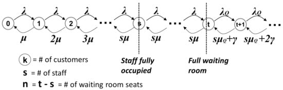
Figure 1.
Deferred abandonment model (reneging system).
We consider two systems: reneging system and balking system. For the reneging system, we assume exponential reneging with rate . For the balking system, we assume that the arrival rate drops by a linear balking rate for each additional customer in queue. For either system, we allow changes in arrival and service rates when there is a queue that incurs abandonment, and denote these rates as and , respectively. (Thus, constant balking is incorporated in both (exponential) reneging and (linear) balking systems.) Let reneging/balking start at state , where s is the number of staff. The birth and death coefficients of the Markov chain representing the deferred abandonment model are as follows:
- 1.
- For the reneging system, the total arrival rate and the total service rate at state k areand .
- 2.
- For the balking system, the total arrival rate and the total service rate at state k areand .Note: denotes a positive part of a function.
Our deferred abandonment model can represent either the (exponential) reneging system () or the (linear) balking system (), both of which incorporate buffer spaces (), constant balking (), and change of server speed (any ). Our model is reduced to the original Erlang A/B/C models by choosing parameters appropriately. For example, if we set (), (thus ), and , then our model becomes the standard Erlang A model (M/M/s+M queue). If when , our model approaches the Erlang C model (M/M/s queue). Finally, if and (thus ), our model becomes the Erlang B model (M/M/s/s queue).
Before concluding this section, we define several parameters to simplify the presentation of this paper. We define the resource requirement of sub-chain 1 as and the resource requirement of sub-chain 2 as . In this paper, we assume (because facility managers always try to reduce the level of congestion when the system is congested). We define linear and square-root staffing coefficients as and , respectively. Server utilization is defined as . We also define . Other symbols are defined as needed throughout the paper.
3. Analysis of the Deferred Abandonment Model
We define the following performance indicators: is the probability that a customer enters a queue with abandonment (reneging or balking) (i.e., ); is the probability that customers abandon a queue via constant balking or exponential reneging (for the reneging system), or abandon a queue via constant balking or linear balking (for the balking system); is the probability that an arriving customer sits in one of the n seats in the buffer space (i.e., ). (Note: when .) We define the delay probability for this system as . We represent these performance indicators by the blocking probabilities of three truncated sub-chains: and . For this purpose, we utilize Kelly’s property (Corollary 1.10. in [11]) that holds for a reversible Markov chain. (Note: The extension of the property to more general Markov chains is discussed in [12].) Since our deferred abandonment model is a reversible Markov chain, the entire Markov chain and its truncated sub-chains satisfy Kelly’s property:
Lemma 1.
(Kelly‘s property). Suppose that a Markov chain is reversible. Let be the probability that we observe a state in sub-chain i. holds for any sub-chain i and any state k in sub-chain i.
The proof of Lemma 1 is omitted (see [11] or [12] if interested.) Lemma 1 essentially states that a truncated sub-chain has the same stationary distribution as the distribution of the entire Markov chain given in the sub-chain. Lemma 1 allows us to work on the individual truncated sub-chain rather than on the entire Markov chain, simplifying the analysis of Markov chain models substantially. Using Lemma 1 repeatedly, we can derive the exact relationships among performance indicators and blocking probabilities, which are summarized in Lemma 2.
Lemma 2.
The following structural representation holds for the deferred abandonment model:
where
and
Proof of Lemma 2.
We denote the sub-chain that combines sub-chain 3 and sub-chain 2 as sub-chain 2+. By viewing chain 2+ as the entire chain and chain 3 as a sub-chain of chain 2+, we can apply Lemma 1 to states s and t that belong to sub-chain 2+, and obtain the relationship , from which we obtain . Additionally, using Lemma 1, we can show
from which we obtain
and likewise,
Combining these results, we can derive :
We can also derive and using Lemma 1:
and
Finally, notice that the abandonment occurs only at the reneging/balking sub-chain (i.e., sub-chain 2) and the probability of abandonment given sub-chain 2 is . Thus, using Lemma 1 again, we obtain
where
□
Remark 1.
By plugging the exact, approximate, or asymptotic limit of blocking probabilities and into Lemma 2, we can derive the exact, approximate, or asymptotic limit of performance indicators for the deferred abandonment model, respectively.
For the rest of this section, we show that the two important indicators, the delay probability and the abandonment probability , exhibit a trade-off relationship when the number of buffer spaces n changes. For this purpose, we denote performance indicators of the deferred abandonment model as an explicit function of n: , , , , and . When , sub-chain 3 is reduced to a single state s; thus, , , , and hold. To simplify the representation, we introduce functions and that represent delay and abandonment probabilities for the Markov chain model which comprises two of the three sub-chains in the deferred abandonment model: sub-chains 1 and 2, sub-chains 1 and 3, or sub-chains 3 and 2. (Note: Abandonment probability is defined properly only when the right sub-chain is sub-chain 2.) When , the model is composed of sub-chains 1 and 2, and thus,
To prove the trade-off relationship between and , the following lemma is necessary.
Lemma 3.
For any (i.e., ) for the deferred abandonment model, the following inequalities hold:
Proof of Lemma 3.
For the first relationship, consider the case only, since the relationship is trivial when . Assuming , the first relationship is equivalent to . Note that from the definitions of arrival/service rates for the left sub-chain, , , , and hence, , where the equality holds only at . Notice also that when . Using these properties and the exact result, we can derive the first relationship:
Next, for the second relationship, consider the case only, since the relationship is trivial when . Assuming , the second relationship is equivalent to . Note that from the definitions of arrival/service rates for the right (reneging/balking) part of the Markov chain, , , , and hence, , where the equality would hold when both and hold. (Note that the equality does not hold since we assume that reneging/balking must exist.) Notice also that when . Using these properties and the exact result, we can derive the second relationship:
□
Using Lemma 3 and performance indicators and for the two sub-chain model, we can now prove the trade-off relationship between and .
Proposition 1.
For the deferred abandonment system, and show the trade-off relationship as n changes.
- 1.
- monotonically increases as n increases:The lower bound is at and the upper bound is either , (when ) or 1 (when ) at .
- 2.
- monotonically decreases as n increases:The upper bound is at and the lower bound is either 0 (when ) or (when ) at .
Remark 2.
In Proposition 1, performance indicators of the two sub-chain model (i.e., and ) show up; this is explained intuitively as follows: When sub-chain 3 (middle sub-chain) does not exist (), the deferred abandonment model with three sub-chains (left, middle, and right) becomes the model with only sub-chains 1 and 2 (left and right). Likewise, when sub-chain 3 is infinitely large (), the deferred abandonment model becomes equivalent to the model with either sub-chains 1 and 3 (left and middle) if , or sub-chains 3 and 2 (middle and right) if . Since the upper/lower bounds of and are obtained at either or , the properties of the deferred abandonment model can be described by the properties of the two sub-chain model. Note that the following properties hold for sub-chain 3: at when (thus and ) and at when (thus and ).
Proposition 1 indicates that the trade-off relationship exists between and . If we provide more seats for customers in a buffer space in an abandonment system, we are able to reduce the number of customers abandoning the system (i.e., reduce ) at the cost of higher delay probability for arriving customers (i.e., increase ). For the remainder of this section, we show the proof of Proposition 1.
Proof of Proposition 1.
For the deferred abandonment model, we assume that sub-chain 3 is an M/M/1/n queue with . We consider two possible cases: (1) and (2) . For the second case, we utilize Lemma 3.
(1) : In this case, sub-chain 3 (an M/M/1/n queue with ) satisfies
Combined with Lemma 2, we obtain
from which we obtain
This result obviously satisfies the properties shown in Proposition 1. monotonically increases as n increases; the lower bound is at ; the upper bound is 1 at . monotonically decreases as n increases; the upper bound is at ; the lower bound is 0 at .
(2) : In this case, sub-chain 3 (an M/M/1/n queue with ) satisfies
To obtain a representation in terms of a linear coefficient a, we further rewrite these equations using the relationships, , , and , and we obtain
Combined with Lemma 2, we obtain
from which we obtain
and
As we expect, when , we retrieve and .
To prove that increases monotonically as n increases, notice that is a positive increasing function of n. Regardless of the value of a (note: holds for , and holds for ), using Lemma 3, is a monotonically increasing function of n which satisfies
where the equality holds at . We can conclude that is an increasing function of n where the lower bound is obtained at , and the upper bound is either (when ) or 1 (when ) at .
To prove that decreases monotonically as n increases, notice that is a positive increasing function of n. Regardless of the value of a, using Lemma 3, is a monotonically increasing function of n which satisfies
where the equality holds at . We can conclude that is a decreasing function of n where the the upper bound is obtained at , and the lower bound is either 0 (when ) or (when ) at . □
4. Asymptotic Representation of Systems with Deferred Abandonment
In Proposition 1, we observe that there exists a trade-off relationship between the delay probability and the abandonment probability when the size of the buffer space changes. This is true for any systems with smaller (finite) resource requirement R. However, what if when the system grows large? In fact, many systems exhibit larger R compared to the number of buffer spaces n. In this section, we analyze the asymptotic limit of larger systems, obtain useful linear/square-root staffing rules, and discuss the trade-off relationship for larger systems. To find the asymptotic limit of performance indicators, all we need to know is the asymptotic limit of blocking probabilities for sub-chains 1 and 2 since sub-chain 3 is only affected by n and not by R.
To represent asymptotic results, we first define the necessary parameters in Table 1. For simplicity, we use square-root coefficients , , , and linear coefficients , , , which correspond to sub-chain 1 (M/M/s/s), sub-chain 2 (reneging), and sub-chain 2 (balking), respectively. Following the normal approximation described in [10], we obtain Lemma 4: Blocking probabilities of sub-chains are approximated by the hazard function for the standard normal distribution and the continuity correction terms , , and .

Table 1.
Definition of parameters.
Lemma 4.
Blocking probabilities of sub-chain 1 (M/M/s/s sub-chain) and sub-chain 2 (reneging or balking sub-chain) are approximately represented using the standard normal hazard function :
We omit the proof of Lemma 4, as it is almost identical to that given in [10]. The key idea of this approximation is to represent blocking probabilities of sub-chains by the Poisson representation, and approximate them by the standard normal representation. The averages of the three Poisson distributions for sub-chains 1, 2 (reneging), and 2 (balking) when blocking probabilities are represented by the Poisson random variables are R, and , and the continuity correction terms when converting the discrete Poisson distribution to the continuous standard normal distribution are , , and , respectively. The Poisson-to-normal approximation is elementary, but highly accurate when the average of the Poisson distribution is around 10 or more, and the approximation becomes exact when the average goes to infinity. Thus, Lemma 4 accurately represents the blocking probabilities of all sub-chains as (which leads to as well). We now obtain two asymptotic limits of blocking probabilities: (i) linear staffing rule (when ); and (ii) square-root staffing rule (when ).
Lemma 5
(Linear staffing asymptotic regime). Let (or ) and take the limit of large R with fixed a. Then
- 1.
- For sub-chain 1 (M/M/s/s sub-chain)
- 2.
- For sub-chain 2 (either reneging or balking sub-chain)
Proof of Lemma 5.
We use the properties of the standard normal hazard function in this proof: as and as . Now, consider taking the limit of large R while fixing . For sub-chain 1, if (i.e., ), then , and thus, as ; and if (i.e., ), then , and thus, as .
For sub-chain 2, if (i.e., ), then and , both of which are fixed. Thus, and , leading to as . (Note that as ; see Table 1) Likewise, if (i.e., ), then and . Thus, and , leading to (or ) as . □
Lemma 6
(Square-root staffing asymptotic regime). Assume (thus, ). Let (or ) and . By taking the limit of large R with fixed c, we obtain:
- 1.
- For sub-chain 1 (M/M/s/s sub-chain)
- 2.
- For sub-chain 2 (either reneging or balking sub-chain)where (or δ) for reneging (or balking) sub-chain.
Proof of Lemma 6.
We take the limit of large R while fixing . Thus, . Additionally, using Table 1 and the assumption (thus ), we obtain , , , and . Finally, all continuity correction terms become negligible in the limit of large R: . Combining these results with Lemma 4, we obtain the result of Lemma 6. □
Combining Lemmas 2, 5 and 6 with the assumption , we obtain Proposition 2. Proposition 2 describes the asymptotic representation of performance indicators given n (or more specifically, we take the limit of large R while fixing n). Notice that the case (thus, holds) corresponds to the asymptotic formulae for the Erlang A model. We define a function needed for the square-root staffing rule: , where (or ) for a reneging (or balking) system.
Proposition 2.
We consider three asymptotic regimes for the deferred abandonment model:
- 1.
- ED asymptotic regime: We take the limit of large R while fixing the linear coefficient a that satisfies and obtain
- 2.
- QD asymptotic regime: We take the limit of large R while fixing the linear coefficient a that satisfies and obtain
- 3.
- QED asymptotic regime: There are two QED asymptotic regimes.
- (a)
- (Linear staffing rule) When , we take the limit of large R while fixing the linear coefficient a that satisfies and obtain
- (b)
- (Square-root staffing rule) When (thus, ), we take the limit of large R while fixing the square-root coefficient c that satisfies and obtain
Proof of Proposition 2.
Following the linear staffing representation, it is easy to analyze two extreme cases: (ED regime) and (QD regime). Using Lemmas 2 and 5, we obtain , , , for the ED regime; and , , , for the QD regime.
We next consider the QED regime that exists in between the two extreme (ED and QD) regimes. If , the linear staffing rule following can achieve the QED regime. The properties of this QED regime are obtained using Lemmas 2 and 5: , , , and . (We omit the calculation since it is straightforward, although cumbersome.)
If (i.e., ), two extreme regimes are adjacent in the linear staffing representation. Thus, we utilize the finer square-root staffing representation to describe the properties of the QED regime that exists at the boundary of the ED and QD regimes. Using Lemmas 2 and 6, we obtain , , , and . □
Proposition 2 shows that there is no trade-off between the delay probability () and the abandonment probability () in the asymptotic limit of R. In the two extreme regimes, ED and QD, both and do not depend on n, implying that the number of seats n in the buffer space does not impact the performance indicators. For the QED regime that exists in between the two extreme regimes, we consider two scenarios: (1) if , the linear staffing rule applies and tells us that as n increases, could increase (since , , and ); and (2) if , the square-root staffing rule applies and tells us that is not affected by n. remains the same as n increases for both scenarios. We conclude that providing a buffer space would not be beneficial in the asymptotic limit, which is in contrast to the non asymptotic limit case (Proposition 1).
5. Conclusions
We propose a queueing model with customer abandonment (reneging/balking) that incorporates a buffer space. We call this model the deferred abandonment model. We derive asymptotic formulae for performance indicators: the delay probability and the abandonment probability. We find that the provision of the buffer space may be worthwhile for smaller systems, but is not beneficial and in fact could be harmful for larger systems. This is because the buffer space may only exacerbate the delay probability without improving the throughput of the facility in an asymptotic limit.
Funding
This research received no external funding.
Institutional Review Board Statement
Not applicable.
Informed Consent Statement
Not applicable.
Acknowledgments
The author is grateful for the helpful comments and suggestions provided by the review team, which greatly improved the presentation of this paper. The author appreciates Robert Hampshire and Alan Scheller-Wolf for their valuable feedback and support. The author acknowledges Teresa Rainone for her advice on one of the examples used in this paper. The author is also thankful to Mary Glavan and Jasim Ahmed for their helpful revisions of the paper. This paper is dedicated to the memory of Matthew S. for his genuine friendship.
Conflicts of Interest
The author declares no conflict of interest.
References
- Palm, R.C.A. Research on Telephone Traffic Carried by Full Availability Groups; Tele: Stockholm, Sweden, 1957; Volume 1. [Google Scholar]
- Udagawa, K.; Nakamura, G. On a Queue in which Joining Customers Give up Their Services Halfway. J. Ops. Res. Jpn. 1957, 1, 59–76. [Google Scholar]
- Haight, F.A. Queueing with reneging. Metrika 1959, 2, 186–197. [Google Scholar] [CrossRef]
- Ancker, C.; Gafarian, A. Some queuing problems with balking and reneging. I. Oper. Res. 1963, 11, 88–100. [Google Scholar] [CrossRef]
- Dong, J.; Feldman, P.; Yom-Tov, G.B. Service systems with slowdowns: Potential failures and proposed solutions. Oper. Res. 2015, 63, 305–324. [Google Scholar] [CrossRef] [Green Version]
- Azriel, D.; Feigin, P.D.; Mandelbaum, A. Erlang-S: A data-based model of servers in queueing networks. Manag. Sci. 2019, 65, 4607–4635. [Google Scholar] [CrossRef]
- Wu, C.; Bassamboo, A.; Perry, O. Service system with dependent service and patience times. Manag. Sci. 2019, 65, 1151–1172. [Google Scholar] [CrossRef]
- Garnett, O.; Mandelbaum, A.; Reiman, M. Designing a call center with impatient customers. Manuf. Serv. Oper. Manag. 2002, 4, 208–227. [Google Scholar] [CrossRef] [Green Version]
- Mandelbaum, A.; Zeltyn, S. The Palm/Erlang—A Queue, with Applications to Call Centers; Faculty of Industrial Engineering & Management, Technion: Haifa, Israel, 2005. [Google Scholar]
- Sasanuma, K.; Scheller-Wolf, A. Approximate performance measures for a single station two-stage reneging queue. Oper. Res. Lett. 2021, 49, 212–217. [Google Scholar] [CrossRef]
- Kelly, F.P. Reversibility and Stochastic Networks; John Wiley & Sons: New York, NY, USA, 1979. [Google Scholar]
- Sasanuma, K.; Hampshire, R.; Scheller-Wolf, A. Markov chain decomposition based on total expectation theorem. arXiv 2019, arXiv:1901.06780 2019. [Google Scholar]
Publisher’s Note: MDPI stays neutral with regard to jurisdictional claims in published maps and institutional affiliations. |
© 2021 by the author. Licensee MDPI, Basel, Switzerland. This article is an open access article distributed under the terms and conditions of the Creative Commons Attribution (CC BY) license (https://creativecommons.org/licenses/by/4.0/).