Application of Said Ball Curve for Solving Fractional Differential-Algebraic Equations

Abstract

The aim of this paper is to apply the Said Ball curve (SBC) to find the approximate solution of fractional differential-algebraic equations (FDAEs). This method can be applied to solve various types of fractional order differential equations. Convergence theorem of the method is proved. Some examples are presented to show the efficiency and accuracy of the method. Based on the obtained results, the SBC is more accurate than the Bezier curve method.

1. Introduction

Algebraic and differential equations have important roles in many mathematical and engineering problems [1]. Particularly, in recent years, we can find many problems and mathematical models based on fractional calculus (FCs) in the form of fractional order derivatives [1,2,3,4,5,6].

Fractional modeling has become applicable in different sciences during the past three decades or more. In addition, many physical and engineering topics such as dynamics of earthquakes, electromagnetic theory, fluid flow, and viscoelastic materials are related to differential-algebraic equations (DAEs). As we know, in general, form finding the exact solution of FDAEs is impossible. Thus, finding numerical methods for solving these problems is among the challenging topics in applied mathematics.

Applying the classical derivatives, we can discuss the changes in a neighborhood of a point but, in the fractional derivative, we can discuss the changes in an interval. Because of this property, we can model many physical, mathematical and also natural phenomena using the fractional derivative.

By a system of DAEs, many physical problems are governed. The homotopy analysis method (HAM) is among the semi-analytical methods which have been presented by Liao [7]. Zurigat et al. has applied the HAM to solve the class of FDAEs [8]. For more applications of the HAM see [9,10,11,12]. Ford and Connolly [13] and Diethelm et al. [14] have studied many techniques and stated their respective strengths and weaknesses. For numerical and analytical schemes to solve FDEs, the readers can study [15,16,17,18,19,20,21,22].

A cubic polynomial curve described mathematically during the eminent aircraft design system for the conic lofting surface program CONSURF ([23]). It is extended to three further distinct generalizations called Said Ball curves (SBCs), DP Ball curves, and Wang Ball curves for higher degree polynomials.

Some advantages of the Ball functions (BFs) are identified. Cubic BFs can be reduced to the quadratic Bezier curves (BCs) when the interior control point of the BFs combine with the Ball basis function. The BF is more efficient in term of computation when generalized representations of Ball curves is used [24]. Meanwhile, the BF is more competent in terms of computation compared to the BC and the shape preservative construction properties are similar between the Bernstein Bezier basis and the Said Ball basis [24]. For other advantages of the BFs, see [25].

This point is imperative when it comes to data transfer among Computer Aided Design (CAD) systems.

In this paper, the BFs are applied to solve the following FDAEs

$$\begin{array}{ccc}\hfill & & {\mathfrak{D}}^{{\alpha }_i}{x}_i\left(r\right)=f_i(r,x_1,x_2,\dots ,x_n,x_1^{\prime },x_2^{\prime },\dots ,x_n^{\prime }),i=1,2,\dots ,n-1,0<{\alpha }_i\le 1,\hfill \\ & & g(r,x_1,x_2,\dots ,x_n)=0,\hfill \\ & & x_i\left(0\right)=x_{i,0},i=1,2,\dots ,n\hfill \end{array}$$

(1)

where $x_{i,0}$ are given known numbers, also $f_i(..)$ ($i=1,2,\dots ,n-1$) and $g(..)$ are given continues functions.

Some papers have solved this problem [26,27,28]. For example, the numerical solution of FDAEs was considered by Haar wavelet functions [27]. They derived the Haar wavelet operational matrix of the fractional order integration [27]. In [26], the Bezier curves method (BCM) was implemented to give approximate solutions for FDAEs.

Our strategy is utilizing the Said Ball function (SBF) for solving the FDAEs in form (1) by the least square method. The least squares objective function in LSM was developed to find the approximate solutions of FDEs based on the control points of BCM [26].

The remainder of the paper is organized as follows: Basic preliminaries are stated in Section 2. Section 3 introduces the SBCs (Said Ball curves) and their properties. The technique based on the control points of SBF is stated in Section 4. The convergence of SBF is introduced in Section 5. Section 6 states the applicability and accuracy of this method. Finally, in Section 7 conclusions are drawn.

2. Some Preliminaries

In this section, some main definitions of the fractional order derivative are presented.

Definition 1.

The FD of $x\left(r\right)$ in the Caputo sense of a function $x\in C_{\mu }$, $\mu \ge -1$ is defined as

$$\begin{array}{ccc}& & {\mathfrak{D}}^{\alpha }x\left(r\right)=\frac{1}{\mathsf{\Gamma }(n-\alpha )}{\int }_0^r{(r-z)}^{n-\alpha -1}{x}^{\left(n\right)}\left(z\right)dz,\alpha >0,\exists n\in \mathbb{Z},n-1<\alpha \le n.\hfill \end{array}$$

Definition 2.

For $x\in C_{\mu }$, $\mu \ge -1$, the Riemann–Liouville fractional integral operator of order $\alpha \ge 0$ can be defined as follows

$$\begin{array}{ccc}& & I^{\alpha }x\left(r\right)=\frac{1}{\mathsf{\Gamma }\left(\alpha \right)}{\int }_0^r{(r-z)}^{\alpha -1}x\left(z\right)dz,\alpha >0,t>0,\hfill \\ & & I^{0}x\left(r\right)=x\left(r\right).\hfill \end{array}$$

3. The Said Ball Curves

The Said Ball curves (SBCs) with arbitrary degree of m is ${\displaystyle x\left(r\right)=\sum _{j=0}^m{a}_j{B}_j^m\left(r\right)}$ where $a_j$ ($j=0,1,\dots ,m$) are $m+1$ control points. If m is odd, then

$$\begin{array}{ccc}& & B_j^m\left(r\right)=\left\{\begin{array}{cc}\left(\genfrac{}{}{0pt}{}{\frac{m-1}{2}+j}{j}\right)r^j{(1-r)}^{\frac{m-1}{2}+1},\hfill & 0\le j\le \frac{m-1}{2},\hfill \\ \left(\genfrac{}{}{0pt}{}{\frac{m-1}{2}+m-j}{m-j}\right)r^{\frac{m-1}{2}+1}{(1-r)}^{m-j},\hfill & \frac{m+1}{2}\le j\le m,\hfill \end{array}\right.\hfill \end{array}$$

(2)

if m is even, then

$$\begin{array}{ccc}& & B_j^m\left(r\right)=\left\{\begin{array}{cc}\left(\genfrac{}{}{0pt}{}{\frac{m}{2}+j}{j}\right)r^j{(1-r)}^{\frac{m}{2}+1},\hfill & 0\le j\le \frac{m}{2},\hfill \\ \left(\genfrac{}{}{0pt}{}{m}{\frac{m}{2}}\right)r^{\frac{m}{2}}{(1-r)}^{\frac{m}{2}},\hfill & j=\frac{m}{2},\hfill \\ \left(\genfrac{}{}{0pt}{}{\frac{m}{2}+m-j}{m-j}\right)r^{\frac{m}{2}+1}{(1-r)}^{m-j},\hfill & \frac{m}{2}+1\le j\le m.\hfill \end{array}\right.\hfill \end{array}$$

(3)

Some properties of Said Ball function (SBF) are:

• SBF is non-negative

  $$\begin{array}{ccc}& & B_j^m\left(r\right)\ge 0,0\le r\le 1,\hfill \end{array}$$
• Partition of SBF is unity

  $$\begin{array}{ccc}& & \sum _{j=0}^m{B}_j^m\left(r\right)=1,0\le r\le 1.\hfill \end{array}$$

The stated properties of the SBF indicated the convex combination of its control points. Therefore, the SBC is in the convex hull of its control polygon with control points (see [24]).

4. The Technique Based on the Control Points of the SBF

Without lose of generality, we consider the following form:

$$\begin{array}{ccc}& & {\mathfrak{D}}^{{\alpha }_i}x\left(r\right)=f(r,x,x^{\prime }),\hfill \\ & & g(r,x)=0,\hfill \\ & & x\left(0\right)=x_0,\hfill \end{array}$$

(4)

We substitute ${\displaystyle x\left(r\right)=\sum _{j=0}^m{a}_j{B}_j^m\left(r\right)}$ in Equation (5), and we define the following objective functions for control points of SBF:

$$\begin{array}{ccc}& & J_{objective}=\sum _{j=0}^m{a}_j^2.\hfill \end{array}$$

Now, we solve the following constrained optimization problems:

$$\begin{array}{ccc}& & min{J}_{objective}=\sum _{j=0}^m{a}_j^2,\hfill \\ & & suchthat{\mathfrak{D}}^{\alpha }\left(\sum _{j=0}^m{a}_j{B}_j^m\left(r\right)\right)=f\left(r,\sum _{j=0}^m{a}_j{B}_j^m\left(r\right),{\left(\sum _{j=0}^m{a}_j{B}_j^m\left(r\right)\right)}^{\prime }\right),\hfill \\ & & g\left(r,\sum _{j=0}^m{a}_j{B}_j^m\left(r\right)\right)=0,\hfill \\ & & \sum _{j=0}^m{a}_j{B}_j^m\left(0\right)=x_0,\hfill \end{array}$$

where ${\displaystyle {\mathfrak{D}}^{\alpha }\left(\sum _{j=0}^m{a}_j{B}_j^m\left(r\right)\right)}$ is defined in Definition 1.

5. Convergence of the SBF

Suppose that $H=L^2[0,1]$ be the Hilbert space and $\{B_0^m,B_1^m,\dots ,B_m^m\}$ the polynomials of degree m on $[0,1]$ [29]. We define $Y=Span\{B_0^m,B_1^m,\dots ,B_m^m\}$. Assume that x is an arbitrary element in H. We know that Y is a finite dimensional subspace of the space H, thus the best unique approximation $x_m\in Y$ can be found as

$$\begin{array}{ccc}& & \exists x_m\in Y\mathrm{s}.\mathrm{t}.\forall y\in Y,\parallel x-x_m{\parallel }_2\le {\parallel x-y\parallel }_2\hfill \end{array}$$

where ${\parallel x\parallel }_2=⟨x,x⟩$ and $⟨,⟩$ denotes the inner product. Since $x_m\in Y$, $x_m$ is a linear combination of the spanning basis of Y, which means that there are $m+1$ coefficients $A=[a_0,a_1,\dots ,a_m]\in \mathbb{R}$ such that

$$\begin{array}{ccc}& & x\left(r\right)\approx x_m\left(r\right)=\sum _{j=0}^m{a}_j{B}_j^m\left(r\right)=A^T{\varphi }_m\left(r\right),\hfill \end{array}$$

where $\parallel x-x_m{\parallel }_2\to min$, then A can be obtained by $A=W^{-1}⟨x\left(r\right),{\varphi }_m\left(r\right)⟩$, where $W=⟨{\varphi }_m\left(r\right),{\varphi }_m\left(r\right)⟩={\int }_0^1{\varphi }_m\left(r\right){\varphi }_m^T\left(r\right)dr$.

The Proof of the Convergence

We consider the following problem

$$\begin{array}{ccc}& & {\mathfrak{D}}^{\alpha }x\left(r\right)=A_1\left(r\right)\mathfrak{D}x\left(r\right)+B_1\left(r\right)\mathfrak{D}{x}_1\left(r\right)+C_1\left(r\right)x\left(r\right)+G_1\left(r\right)x_1\left(r\right),\hfill \\ & & x_1\left(r\right)=H_1\left(r\right),r\in [0,1],x\left(0\right)=x_0=a,x_1\left(0\right)=x_{1,0}=b,\hfill \end{array}$$

then

$$\begin{array}{c}L\left(x\left(r\right),x_1\left(r\right),{\mathfrak{D}}^{\alpha }x\left(r\right),\mathfrak{D}x\left(r\right),\mathfrak{D}{x}_1\left(r\right)\right)\hfill \\ \\ ={\mathfrak{D}}^{\alpha }x\left(r\right)-\left(A_1\left(r\right)\mathfrak{D}x\left(r\right)+B_1\left(r\right)\mathfrak{D}{x}_1\left(r\right)+C_1\left(r\right)x\left(r\right)+G_1\left(r\right)x_1\left(r\right)\right)=F_1\left(r\right),\hfill \\ \\ x_1\left(r\right)=H_1\left(r\right),r\in [0,1],x\left(0\right)=x_0=a,x_1\left(0\right)=x_{1,0}=b,\hfill \end{array}$$

(5)

where $x\left(r\right),x_1\left(r\right)\in R$ and $a,b$ are given real numbers, and $A_1\left(r\right)$, $B_1\left(r\right)$, $C_1\left(r\right)$, $G_1\left(r\right)$, $H_1\left(r\right)$ and $F_1\left(r\right)$ are known polynomials on $r\in [0,1]$.

Theorem 1.

If $\overline{x}$, ${\overline{x}}_1\in C^1$ are the unique continuous solutions of the problem (5), then the obtained approximate solutions are converge to the exact solution $(\overline{x},{\overline{x}}_1)$.

Proof. 

For $ϵ>0$, by the Weierstrass Theorem [30], we can find the polynomials $W_{1,V_1}\left(r\right)$ and $W_{2,V_2}\left(r\right)$ of degrees $V_1$ and $V_2$ such that

$$\begin{array}{ccc}& & \parallel \frac{d^i{W}_{1,V_1}\left(r\right)}{d{t}^i}-\frac{d^i\overline{x}\left(r\right)}{d{t}^i}{\parallel }_{\infty }\le \frac{ϵ}{16},\hfill \\ & & \parallel \frac{d^i{W}_{2,V_2\left(r\right)}}{d{t}^i}-\frac{d^i\overline{x_1}\left(r\right)}{d{t}^i}{\parallel }_{\infty }\le \frac{ϵ}{16},i=0,1.\hfill \end{array}$$

We note that: ${\parallel .\parallel }_{\infty }$ is the $L_{\infty }$-norm, hence

$$\begin{array}{ccc}\hfill & & \parallel a-W_{1,V_1}{\left(0\right)\parallel }_{\infty }\le \frac{ϵ}{16},\hfill \\ & & \parallel b-W_{2,V_2}{\left(0\right)\parallel }_{\infty }\le \frac{ϵ}{16}.\hfill \end{array}$$

(6)

We know that $W_{1,V_1}\left(r\right)$ and $W_{2,V_2}\left(r\right)$ do not satisfy in the boundary conditions. Thus, making perturbation on $W_{1,V_1}\left(r\right)$ and $W_{2,V_2}\left(r\right)$, the following polynomials are obtained

$$S_{1,V_1}\left(r\right)=W_{1,V_1}\left(r\right)+\beta ,$$

and

$$S_{2,V_2}\left(r\right)=W_{2,V_2}\left(r\right)+\gamma ,$$

where $S_{1,V_1}\left(0\right)=a$ and $S_{2,V_2}\left(0\right)=b$. Therefore $W_{1,V_1}\left(0\right)+\beta =a$ and using Equation (6) we get

$$\begin{array}{ccc}& & \parallel a-W_{1,V_1}{\left(0\right)\parallel }_{\infty }={\parallel \beta \parallel }_{\infty }\le \frac{ϵ}{16}.\hfill \end{array}$$

We obtain $b=S_{2,V_2}\left(0\right)=W_{2,V_2}\left(0\right)+\gamma$, hence

$$\begin{array}{ccc}& & \parallel b-W_{2,V_2}{\left(0\right)\parallel }_{\infty }={\parallel \gamma \parallel }_{\infty }\le \frac{ϵ}{16},\hfill \end{array}$$

so

$$\begin{array}{ccc}\hfill \parallel S_{1,V_1}\left(r\right)-\overline{x}{\left(r\right)\parallel }_{\infty }& =& \parallel W_{1,V_1}\left(r\right)-\overline{x}{\left(r\right)\parallel }_{\infty }\hfill \\ & \le & \parallel W_{1,V_1}\left(r\right)-\overline{x}{\left(r\right)\parallel }_{\infty }+{\parallel \gamma \parallel }_{\infty }\hfill \\ & \le & \frac{ϵ}{8}<\frac{ϵ}{5},\hfill \\ \hfill \parallel \mathfrak{D}{S}_{1,V_1}\left(r\right)-\mathfrak{D}\overline{x}{\left(r\right)\parallel }_{\infty }& =& \parallel \frac{d{S}_{1,V_1}\left(r\right)}{dr}-\frac{d\overline{x}\left(r\right)}{dr}{\parallel }_{\infty }\hfill \\ & =& \parallel \frac{d{W}_{1,V_1}\left(r\right)}{dr}-\frac{d\overline{x}\left(r\right)}{dr}{\parallel }_{\infty }\hfill \\ & <& \frac{3ϵ}{16}<\frac{ϵ}{5},\hfill \\ \hfill \parallel {\mathfrak{D}}^{\alpha }{S}_{1,V_1}\left(r\right)-{\mathfrak{D}}^{\alpha }\overline{x}{\left(r\right)\parallel }_{\infty }& \le & |\frac{1}{\mathsf{\Gamma }(m-\alpha )}|{\int }_0^t{\parallel {(r-z)}^{m-\alpha -1}\parallel }_{\infty }\hfill \\ & \times & \parallel W_{1,V_1}^{\left(m\right)}\left(z\right)-{\overline{x}}^{\left(m\right)}{\left(z\right)\parallel }_{\infty }dz\hfill \\ & \le & |\frac{1}{\mathsf{\Gamma }(m-\alpha )}|\underset{0\le z\le 1}{max}\left|{(r-z)}^{m-\alpha -1}\right|\hfill \\ & \times & \frac{ϵ\mathsf{\Gamma }(m-z)}{16{max}_{0\le z\le 1}\left({|(r-z)}^{m-\alpha -1}|+1\right)}\hfill \\ & \le & \frac{ϵ}{16}<\frac{ϵ}{5},\hfill \end{array}$$

$$\begin{array}{ccc}\hfill \parallel S_{2,V_2}\left(r\right)-{\overline{x}}_2{\left(r\right)\parallel }_{\infty }& =& \parallel W_{2,V_2}\left(r\right)-{\overline{x}}_2{\left(r\right)\parallel }_{\infty }\hfill \\ & \le & \parallel W_{2,V_2}\left(r\right)-{\overline{x}}_2{\left(r\right)\parallel }_{\infty }+{\parallel \gamma \parallel }_{\infty }\hfill \\ & \le & \frac{ϵ}{8}<\frac{ϵ}{5},\hfill \\ \hfill \parallel \mathfrak{D}{S}_{2,V_2}\left(r\right)-\mathfrak{D}{\overline{x}}_2{\left(r\right)\parallel }_{\infty }& =& \parallel \frac{S_{2,V_2}\left(r\right)}{dr}-\frac{d{\overline{x}}_2\left(r\right)}{dr}{\parallel }_{\infty }\hfill \\ & \le & \parallel \frac{d{W}_{2,V_2}\left(r\right)}{dr}-\frac{d{\overline{x}}_2\left(r\right)}{dr}{\parallel }_{\infty }+{\parallel \gamma \parallel }_{\infty }\hfill \\ & \le & \frac{ϵ}{8}<\frac{ϵ}{5}.\hfill \end{array}$$

Assume that

$$\begin{array}{c}L{S}_V\left(r\right)=L\left(S_1,V_1\left(r\right),S_2,V_2\left(r\right),{\mathfrak{D}}^{\alpha }{S}_1,V_1\left(r\right),\mathfrak{D}{S}_{1,V1}\left(r\right),\mathfrak{D}{S}_{2,V_2}\left(r\right)\right)\hfill \\ \\ =\mathfrak{D}{S}_{1,V_1}\left(r\right)-A_1\left(r\right)\mathfrak{D}{S}_{1,V_1}\left(r\right)-B_1\left(r\right)\mathfrak{D}{S}_{2,V_2}\left(r\right)-C_1\left(r\right)S_{1,V_1}\left(r\right)-G_1\left(r\right)S_{2,V_2}\left(r\right)=F_1\left(r\right),\hfill \end{array}$$

thus $V\ge max\{V_1,V_2\}$ and we have

$$\begin{array}{ccc}\hfill \parallel L{S}_V\left(r\right)-F_1{\left(r\right)\parallel }_{\infty }& =& \parallel L(S_{1,V_1}\left(r\right),S_{2,V_2}\left(r\right),{\mathfrak{D}}^{\alpha }{S}_{1,V_1}\left(r\right),\mathfrak{D}{S}_{1,V_1}\left(r\right),\mathfrak{D}{S}_{2,V_2}\left(r\right))-F_1{\left(r\right)\parallel }_{\infty }\hfill \\ & \le & \parallel {\mathfrak{D}}^{\alpha }{S}_{1,V_1}\left(r\right)-{\mathfrak{D}}^{\alpha }\overline{x}{\left(r\right)\parallel }_{\infty }\hfill \\ & +& \parallel A_1{\left(r\right)\parallel }_{\infty }{\parallel \mathfrak{D}{S}_{1,V_1}\left(r\right)-\mathfrak{D}\overline{x}\left(r\right)\parallel }_{\infty }\hfill \\ & +& \parallel B_1{\left(r\right)\parallel }_{\infty }{\parallel \mathfrak{D}{S}_{2,V_2}\left(r\right)-\mathfrak{D}{\overline{x}}_1\left(r\right)\parallel }_{\infty }\hfill \\ & +& \parallel C_1{\left(r\right)\parallel }_{\infty }{\parallel S_{1,V_1}\left(r\right)-\overline{x}\left(r\right)\parallel }_{\infty }\hfill \\ & +& \parallel G_1{\left(r\right)\parallel }_{\infty }{\parallel S_{2,V_2}\left(r\right)-{\overline{x}}_1\left(r\right)\parallel }_{\infty }\hfill \\ & \le & C_1\left(5\frac{ϵ}{5}\right)=C_1ϵ,\hfill \end{array}$$

where $C_1=1+\parallel A_1{\left(r\right)\parallel }_{\infty }+\parallel B_1{\left(r\right)\parallel }_{\infty }+\parallel C_1{\left(r\right)\parallel }_{\infty }+{\parallel G_1\left(r\right)\parallel }_{\infty }$ is a constant. We know $R\left(S_V\right):=L{S}_V\left(r\right)-F_1\left(r\right)$ is a polynomial, we have

$$\begin{array}{ccc}& & R\left(S_V\right)=\sum _{i=0}^{m_1}{d}_{i,m_1}{B}_i^{m_1}\left(r\right),\hfill \end{array}$$

hence, there exists an integer M($\ge V$) where for $m_1>M$, we can write

$$\begin{array}{ccc}\hfill \frac{1}{m+1}\sum _{i=0}^{m_1}{d}_{i,m_1}^2& <& ϵ+{\int }_0^1{\left(R\left(S_V\right)\right)}^{2}dr\hfill \\ & \le & ϵ+C_1^2{ϵ}^2.\hfill \end{array}$$

Suppose $x\left(r\right)$ and $x_1\left(r\right)$ are approximated solution of (5), for $m_2$ ($m_2\ge m_1\ge M$)

$$\begin{array}{ccc}& & R(x\left(r\right),x_1\left(r\right),{\mathfrak{D}}^{\alpha }x\left(r\right),\mathfrak{D}x\left(r\right),\mathfrak{D}{x}_1\left(r\right))\hfill \\ & & =L(x\left(r\right),x_1\left(r\right),{\mathfrak{D}}^{\alpha }x\left(r\right),\mathfrak{D}x\left(r\right),\mathfrak{D}{x}_1\left(r\right))-F_1\left(r\right)\hfill \\ & & =\sum _{i=0}^{m_2}{c}_{i,m_2}{B}_i^{m_2}\left(r\right),\hfill \end{array}$$

then

$$\begin{array}{ccc}\hfill \parallel \left(x\left(r\right),x_1\left(r\right)\right)-\left(\overline{x}\left(r\right),{\overline{x}}_1\left(r\right)\right){\parallel }^2& =& {\int }_0^1{|{\mathfrak{D}}^{\alpha }x\left(r\right)-{\mathfrak{D}}^{\alpha }\overline{x}\left(r\right)|}^{2}dr\hfill \\ & +& {\int }_0^1\sum _{j=0}^1{|\frac{d^{j}x\left(r\right)}{d{r}^j}-\frac{d^j\overline{x}\left(r\right)}{d{r}^j}|}^{2}dr\hfill \\ & +& \sum _{j=0}^1{|\frac{d^j{x}_1\left(r\right)}{d{r}^j}-\frac{d^j{\overline{x}}_1\left(r\right)}{d{r}^j}|}^{2}dr,\hfill \end{array}$$

because

$$\begin{array}{ccc}& & \parallel \left(x\left(r\right),x_1\left(r\right)\right)-\left(\overline{x}\left(r\right),{\overline{x}}_1\left(r\right)\right){\parallel }^2\le C\left(\right|x\left(0\right)-\overline{x}\left(0\right)|+|x_1\left(0\right)-{\overline{x}}_1\left(0\right)|\hfill \\ & & +\parallel R\left((x\left(r\right),x_1\left(r\right),{\mathfrak{D}}^{\alpha }x\left(r\right),\mathfrak{D}x\left(r\right),\mathfrak{D}{x}_1\left(r\right))-(\overline{x}\left(r\right),{\overline{x}}_1\left(r\right),{\mathfrak{D}}^{\alpha }\overline{x}\left(r\right),\mathfrak{D}\overline{x}\left(r\right),\mathfrak{D}{\overline{x}}_1\left(r\right))\right){\parallel }_2^2)\hfill \\ & & =C{\int }_0^1\sum _{i=0}^{m_2}{\left(c_{i,m_2}{B}_i^{m_2}\left(r\right)\right)}^{2}dr\hfill \\ & & \le \frac{C}{m_2+1}\sum _{i=0}^k{c}_{i,m_2}^2,\hfill \end{array}$$

hence

$$\begin{array}{ccc}\hfill \parallel \left(x\left(r\right),x_1\left(r\right)\right)-\left(\overline{x}\left(r\right),{\overline{x}}_1\left(r\right)\right){\parallel }^2& \le & \frac{C}{m_2+1}\sum _{i=0}^{m_2}{c}_{i,m_2}^2\hfill \\ & \le & \frac{C}{m_2+1}\sum _{i=0}^{m_2}{d}_{i,m_2}^2\hfill \\ & \le & \frac{C}{m_1+1}\sum _{i=0}^{m_1}{d}_{i,m_1}^2\hfill \\ & \le & C(ϵ+C_1^2{ϵ}^2)={ϵ}_2.\hfill \end{array}$$

Now, the proof is complete. □

6. Numerical Examples

In this section, we consider some numerical examples to show the efficiency of the method. Furthermore, the numerical results are compared with the Bezier curve method. The results are obtained applying the Maple 14.

Example 1.

Consider the following problem [26,27]:

$$\begin{array}{ccc}& & {\mathfrak{D}}^{\alpha }x\left(r\right)+x\left(r\right)-y\left(r\right)=-sin\left(r\right),\hfill \\ & & x\left(r\right)+y\left(r\right)=e^{-r}+sin\left(r\right),\hfill \\ & & x\left(0\right)=1,y\left(0\right)=0,\hfill \\ & & x_{exact}=e^{-r},y_{exact}=sin\left(r\right),for\alpha =1.\hfill \end{array}$$

This example is solved using the stated method for $\alpha =0.75$. Table 1 shows the numerical results of the example. We note that the absolute error is obtained from the difference of exact ($\alpha =1$) and approximate solutions ($\alpha =0.75$). The computational time to find the results for the SBC is $0.434$ and for the Bezier curve method is $0.438$.

Table 1. Numerical results of Example 1 for various t.

r	Error $\mathit{x}\left(\mathit{r}\right)$	Error $\mathit{y}\left(\mathit{r}\right)$	Error $\mathit{x}\left(\mathit{r}\right)$ in [26]	Error $\mathit{y}\left(\mathit{r}\right)$ [26]
$0.1$	$0.01391401136$	$0.004183397050$	$0.01307884066$	$0.005442098498$
$0.2$	$4\times {10}^{-11}$	$0.0$	$0.01800912414$	$0.007186495790$
$0.3$	$0.002462239190$	$0.009682662$	$0.01624814654$	$0.006220727630$
$0.4$	$0.0$	$0.01084786350$	$0.009558274900$	$0.003512496100$
$0.5$	$0.0$	$0.0$	$0.0\times {10}^{-10}$	$1\times {10}^{-10}$
$0.6$	$0.002383492300$	$0.01322212550$	$0.01008137720$	$0.003417438100$
$0.7$	$0.01698092$	$0.01505722$	$0.01807508510$	$0.005888358900$
$0.8$	$0.04253620650$	$0.00082677884$	$0.02112983790$	$0.006617673400$
$0.9$	$0.05332808630$	$0.05332808630$	$0.01618393680$	$0.004874606600$

Example 2.

One may consider the following problem [26]:

$$\begin{array}{ccc}& & {\mathfrak{D}}^{\alpha }x\left(r\right)-r\mathfrak{D}y\left(r\right)+x\left(r\right)-(1+r)y\left(r\right)=0,\hfill \\ & & y\left(r\right)-sin\left(r\right)=0,\hfill \\ & & x\left(0\right)=1,y\left(0\right)=0,\hfill \\ & & x_{exact}=e^{-t}+tsin\left(r\right),y_{exact}=sin\left(r\right),for\alpha =1.\hfill \end{array}$$

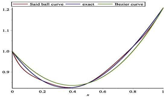
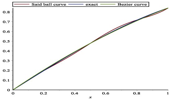
This example is solved by using the stated method with $\alpha =0.75$. The absolute error is presented in Table 2. We note that the absolute error is obtained from the difference of the exact solution for $\alpha =1$ and the approximate solution for $\alpha =0.75$. The graphs of the Said Ball, exact and Bezier curve for $x\left(r\right)$ and $y\left(r\right)$ are shown in Figure 1 and Figure 2 for $\alpha =0.75$. The computational time of the SBC, and the Bezier curve are, respectively, $0.433$ and $0.437$.

Table 2. The absolute errors of $x\left(r\right)$ and $y\left(r\right)$.

r	Error $\mathit{x}\left(\mathit{r}\right)$	Error $\mathit{y}\left(\mathit{r}\right)$
$0.1$	$0.01345302853$	$0.004183397050$
$0.2$	$0.0$	$0.0$
$0.3$	$0.003105586446$	$0.00968266200$
$0.4$	$0.0$	$0.010847886350$
$0.5$	$3.6787\times {10}^{-10}$	$0.0$
$0.6$	$0.003947039374$	$0.01322212550$
$0.7$	$0.005528561954$	$0.01505722$
$0.8$	$0.0$	$0.0008267884$
$0.9$	$0.007268923556$	$0.0150980412$

Figure 1. The graphs of Siad Ball, exact, Bezier curve for $x\left(r\right)$ of Example 2.

Figure 2. The graphs of Siad Ball, exact, Bezier curve for $y\left(r\right)$ of Example 2.

Example 3.

Consider the following problem [31]:

$$\begin{array}{ccc}& & {\mathfrak{D}}^{\alpha }x\left(r\right)=1+2x\left(r\right)-{\left(x\left(r\right)\right)}^2,\hfill \\ & & x\left(0\right)=0,\hfill \\ & & x_{exact}=1+\sqrt{2}tanh\left(\sqrt{2}t+\frac{1}{2}ln\left(\frac{\sqrt{2}-1}{\sqrt{2}+1}\right)\right),for\alpha =1.\hfill \end{array}$$

We solve the problem using the mentioned method for $\alpha =0.75$. The numerical results are presented in Table 3. The results are obtained from the difference of the exact ($\alpha =1$) and approximate solutions ($\alpha =0.75$). The computational time of the SBC, and the Bezier curve are, respectively, $0.431$ and $0.435$.

$$\begin{array}{ccc}\hfill x_{approx}\left(r\right)& =& 8.82312663415527\times {10}^{-9}r{(1-r)}^4\hfill \\ & -& 5.34368571679517\times {10}^{-8}{r}^2{(1-r)}^4\hfill \\ & +& 4.66950466964230\times {10}^{-7}{r}^4{(1-r)}^3\hfill \\ & -& 2.68981346427866\times {10}^{-7}{r}^4{(1-r)}^2\hfill \\ & +& 3.56483520872054\times {10}^{-8}{r}^4(1-r)\hfill \\ & +& 4.11389403714848\times {10}^{-17}{r}^4.\hfill \end{array}$$

Table 3. The absolute errors of $x\left(r\right)$ for Example 3.

r	Error $\mathit{x}\left(\mathit{r}\right)$
$0.1$	$1.7\times {10}^{-9}$
$0.2$	$1.5\times {10}^{-9}$
$0.3$	$1.7\times {10}^{-9}$
$0.4$	$1.7\times {10}^{-9}$
$0.5$	$1.7\times {10}^{-9}$
$0.6$	$1.7\times {10}^{-9}$
$0.7$	$1.7\times {10}^{-9}$
$0.8$	$1.7\times {10}^{-9}$
$0.9$	$8\times {10}^{-10}$

7. Conclusions

In this study, an efficient algorithm based on the SBF was discussed to solve the mentioned FDAEs. The main idea of the method is to adopt the SBF as a new approximation instrument. Finding the control parameters, the approximate solution of the problem was obtained. The validity of the stated method which is based on the SBF was verified by proving the convergence theorem. The efficiency of the method was stated by means of some numerical examples. The comparative study shows the efficiency and accuracy of the SBC than the Bezier curve method. Furthermore, we have an acceptable computational cost for the SBC. Solving linear and nonlinear integral equations of the first and second kinds using the mentioned method is among our future plans.

References

- Shiri, B.; Baleanu, D. System of fractional differential algebraic equations with applications. Chaos Solitons Fractals 2019, 120, 203–212. [Google Scholar] [CrossRef]
- Noeiaghdam, S.; Dreglea, A.; Isik, H.; Suleman, M. Comparative Study between Discrete Stochastic Arithmetic and Floating-Point Arithmetic to Validate the Results of Fractional Order Model of Malaria Infection. Mathematics 2021, 9, 1435. [Google Scholar] [CrossRef]
- Noeiaghdam, S.; Micula, S.; Nieto, J.J. Novel Technique to Control the Accuracy of a Nonlinear Fractional Order Model of COVID-19: Application of the CESTAC Method and the CADNA Library. Mathematics 2021, 9, 1321. [Google Scholar] [CrossRef]
- Noeiaghdam, S.; Micula, S. Dynamical Strategy to Control the Accuracy of the Nonlinear Bio-mathematical Model of Malaria Infection. Mathematics 2021, 9, 1031. [Google Scholar] [CrossRef]
- Hedayati, M.; Ezzati, R.; Noeiaghdam, S. New Procedures of a Fractional Order Model of Novel coronavirus (COVID-19) Outbreak via Wavelets Method. Axioms 2021, 10, 122. [Google Scholar] [CrossRef]
- Noeiaghdam, S.; Sidorov, D. Caputo-Fabrizio Fractional Derivative to Solve the Fractional Model of Energy Supply-Demand System. Math. Model. Eng. Probl. 2020, 7, 359–367. [Google Scholar] [CrossRef]
- Liao, S.J. The Proposed Homotopy Analysis Technique for the Solution of Nonlinear Problems. Ph.D. Thesis, Shanghai Jiao Tong University, Shanghai, China, 1992. [Google Scholar]
- Zurigat, M.; Momani, S.; Alawneh, A. Analytical approximate solutions of systems of fractional algebraic-differential equations by homotopy analysis method. Comput. Math. Appl. 2010, 59, 1227–1235. [Google Scholar] [CrossRef]
- Noeiaghdam, L.; Noeiaghdam, S.; Sidorov, D. Dynamical Control on the Homotopy Analysis Method for Solving Nonlinear Shallow Water Wave Equation. J. Phys. Conf. Ser. 2021, 1847, 012010. [Google Scholar] [CrossRef]
- Noeiaghdam, S.; Fariborzi Araghi, M.A.; Abbasbandy, S. Finding optimal convergence control parameter in the homotopy analysis method to solve integral equations based on the stochastic arithmetic. Numer. Algorithms 2019, 81, 237–267. [Google Scholar] [CrossRef]
- Fariborzi Araghi, M.A.; Noeiaghdam, S. A novel technique based on the homotopy analysis method to solve the first kind Cauchy integral equations arising in the theory of airfoils. J. Interpolat. Approx. Sci. Comput. 2016, 2016, 1–13. [Google Scholar] [CrossRef][Green Version]
- Noeiaghdam, S.; Zarei, E.; Barzegar Kelishami, H. Homotopy analysis transform method for solving Abel’s integral equations of the first kind. Ain Shams Eng. J. 2016, 7, 483–495. [Google Scholar] [CrossRef]
- Ford, N.J.; Connolly, J.A. Comparison of numerical methods for fractional differential equations. Commun. Pure Appl. Anal. 2006, 5, 289–307. [Google Scholar]
- Diethelm, K.; Ford, J.M.; Ford, N.J.; Weilbeer, M. Pitfalls in fast numerical solvers for fractional differential equations. J. Comput. Appl. Math. 2006, 186, 482–503. [Google Scholar] [CrossRef]
- Agrawal, O.P.; Kumar, P. Comparison of five numerical schemes for fractional differential equations. In Advances in Fractional Calculus; Springer: Dordrecht, The Netherlands, 2007; pp. 43–60. [Google Scholar]
- Diethelm, K.; Ford, N.J.; Freed, A.D.; Luchko, Y. Algorithms for the fractional calculus: A selection of numerical methods. Comput. Methods Appl. Mech. Eng. 2005, 194, 743–773. [Google Scholar] [CrossRef]
- Esmaeili, S.; Shamsi, M. A pseudo-spectral scheme for the approximate solution of a family of fractional differential equations. Commun. Nonlinear Sci. Numer. Simul. 2011, 16, 3646–3654. [Google Scholar] [CrossRef]
- Garrappa, R.; Popolizio, M. On accurate product integration rules for linear fractional differential equations. J. Comput. Appl. Math. 2011, 235, 1085–1097. [Google Scholar] [CrossRef]
- Ghoreishi, F.; Yazdani, S. An extension of the spectral Tau method for numerical solution of multi-order fractional differential equations with convergence analysis. Comput. Math. Appl. 2011, 61, 30–43. [Google Scholar] [CrossRef]
- Ma, W.-X. N-soliton solutions and the Hirota conditions in (1+1)-dimensions. Int. J. Nonlinear Sci. Numer. Simul. 2021. [Google Scholar] [CrossRef]
- Ma, W.X. N-soliton solutions and the Hirota conditions in (2+1)-dimensions. Opt. Quantum Electron. 2020, 52, 511. [Google Scholar] [CrossRef]
- Yang, J.Y.; Ma, W.X. Khalique, C.M. Determining lump solutions for a combined soliton equation in (2+1)-dimensions. Eur. Phys. J. Plus 2020, 135. [Google Scholar] [CrossRef]
- Ball, A.A. CONSURF. Part two: Description of the algorithms. Comput. Aided Des. 1975, 7, 237–242. [Google Scholar] [CrossRef]
- Hu, S.M.; Wang, G.Z.; Jin, T.G. Properties of two types of generalized Ball curves. Comput. Aided Des. 1996, 28, 125–133. [Google Scholar] [CrossRef]
- Said, H.B. Generalized Ball curve and its recursive algorithm. ACM Trans. Graph. 1989, 8, 360–371. [Google Scholar] [CrossRef]
- Ghomanjani, F. A new approach for solving fractional differential-algebraic equations. J. Taibah Univ. Sci. 2017. [Google Scholar] [CrossRef]
- Karabacak, M.; Celik, E. The numerical solution of fractional differential-algebraic equations (FDAEs) by Haar wavelet functions. Int. J. Eng. Appl. Sci. 2015, 2, 2394–3661. [Google Scholar]
- Karabacak, M.; Celik, E. The numerical solution of fractional differential-algebraic equations (FDAEs). New Trends Math. Sci. 2013, 1, 1–6. [Google Scholar]
- Kreyszig, E. Introductory Functional Analysis with Applications; John Wiley and Sons: New York, NY, USA, 1978. [Google Scholar]
- Rudin, W. Principles of Mathematical Analysis; McGraw-Hill: New York, NY, USA, 1986. [Google Scholar]
- Esmaeili, S.; Shamsi, M.; Luchko, Y. Numerical solution of fractional differential equations with a collocation method based on Muntz polynomials. Comput. Mathemaics Appl. 2011, 62, 918–929. [Google Scholar] [CrossRef]
Publisher’s Note: MDPI stays neutral with regard to jurisdictional claims in published maps and institutional affiliations. |
© 2021 by the authors. Licensee MDPI, Basel, Switzerland. This article is an open access article distributed under the terms and conditions of the Creative Commons Attribution (CC BY) license (https://creativecommons.org/licenses/by/4.0/).