Schistosomiasis Model Incorporating Snail Predator as Biological Control Agent

Abstract

Schistosomiasis is a parasitic disease caused by the schistosoma worm. A snail can act as the intermediate host for the parasite. Snail-population control is considered to be an effective way to control schistosomiasis spread. In this paper, we discuss the schistosomiasis model incorporating a snail predator as a biological control agent. We prove that the solutions of the model are non-negative and bounded. The existence condition of equilibrium points is investigated. We determine the basic reproduction number when the predator goes to extinction and when the predator survives. The local stability condition of disease-free equilibrium point is proved using linearization, and the Lienard–Chipart and Routh–Hurwitz criteria. We use center-manifold theory to prove the local stability condition of the endemic equilibrium points. Furthermore, we constructed a Lyapunov function to investigate the global stability condition of the disease-free equilibrium points. To support the analytical results, we presented some numerical simulation results. Our findings suggest that a snail predator as a biological control agent can reduce schistosomiasis prevalence. Moreover, the snail-predator birth rate plays an essential role in controlling schistosomiasis spread.

1. Introduction

Schistosomiasis is a parasitic disease caused by schistosoma-worm infection [1]. The parasite has a complicated life cycle. Some types of snail can act as intermediate hosts, while humans and mammals such as cows, pigs, and mice can serve as reservoir hosts [2]. Consequently, the parasite can infect mammals as a human substitute to complete its life cycle. This is one of the several factors that make schistosomiasis very difficult to eradicate. Controlling the snail population is the most effective way to control the spread of schistosomiasis. Some researchers recommended the use of molluscicides to manage the snail host population [1,3,4]. However, molluscicides have some negative environmental effects [5]. Another method that can be used to manage the snail population is an intervention with snail predators or competitors [6,7,8]. Sokolow et al. [7] stated that releasing river prawn, which is a snail predator, into a water contact site can reduce the snail population and schistosomiasis transmission.

Mathematical modeling is used to study the dynamics of the spread of the disease. The first mathematical model that is related to schistosomiasis is discussed in [9]. Schistosomiasis models considering parasite density in the environment are discussed in [10,11,12,13,14]. The authors divided the parasite into two compartments, i.e., miracidiae and cercariae, which can infect snails and humans or mammals, respectively. In 2009, Chiyaka et al. [10] investigated the host–parasite dynamics of schistosomiasis. They proposed a schistosomiasis model that consists of six first-order differential equations. They found that control interventions that target transmission to humans are more effective than control strategies that aim the transmission to snails are. Gao et al. [11] developed a schistosomiasis model to investigate some control strategies, i.e., health education, cercaria control, snail control, and drug treatment. They found that killing snails is the most effective method to manage schistosomiasis spread. Nur et al. [13] proposed a schistosomiasis model incorporating health education and molluscicide intervention. They found that the most effective way to control schistosomiasis prevalence is molluscicide intervention. Moreover, schistosomiasis cannot be eradicated if the only intervention is health education [13]. Diaby et al. [15] proposed a schistosomiasis model with biological control, i.e., competitor-resistant snails. They found that competitor-resistant snails can be used to manage the spread of schistosomiasis. Okamoto et al. [16,17] proposed mathematical models of vectorborne diseases. They found that biological control agents that can be used to control vectorborne diseases are natural predators, natural competitors, or parasites of the vector. Schistosomiasis is a waterborne disease. Hence, we study the dynamics of the spread of schistosomiasis when a snail predator is used as a biological control agent of snails. Different from the model discussed in [10,11,12,13,15,16,17], we propose a schistosomiasis model with a biological control agent of snails, namely, a snail predator.

2. Mathematical Preliminaries

In this section, we present a theorem that can be used to investigate the existence of backward and forward bifurcation. The theorem is very useful, especially in epidemic models. Theorem 1 can be used to investigate the local stability condition of endemic equilibrium [10,11,18]. The proof of Theorem 1 can be found in [19].

Theorem 1

(Castillo-Chavez and Song [19]) Consider the following general system of ordinary differential equations with a parameter ω.

$$\begin{array}{cc}\frac{d\overrightarrow{x}}{dt}=f(\overrightarrow{x},\omega ),\hfill & f:{\mathbb{R}}^n\times \mathbb{R}\to {\mathbb{R}}^n,f\in C^2({\mathbb{R}}^n\times \mathbb{R}),\hfill \end{array}$$

(1)

where 0 is an equilibrium for System (1), such that $f(0,\omega )\equiv 0$ for all ω. Assume

A1:

$JM=D_{x}f(0,0)=\left(\frac{\partial f_i}{\partial x_j}(0,0)\right)$ is the linearization matrix of (1) around equilibrium 0, and ω is evaluated at 0. Zero is a simple eigenvalue of $JM0$, and the other eigenvalues of $JM$ have a negative real part.

A2:

Matrix $JM$ has a right eigenvector $\overrightarrow{v}$ and a left eigenvector $\overrightarrow{w}$ corresponding to the zero eigenvalue. Let $f_k$ be the $kth$ component of f and

$$\begin{array}{c}A={\displaystyle \sum _{k,i,j=1}^n}{w}_k{v}_i{v}_j\frac{{\partial }^2{f}_k\left(0,0\right)}{\partial x_i\partial x_j},\hfill \\ B={\displaystyle \sum _{k,i=1}^n}{w}_k{v}_i\frac{{\partial }^2{f}_k\left(0,0\right)}{\partial x_i\partial \omega }.\hfill \end{array}$$

The dynamics of System (1) around 0 is totally determined by the signs of A and B.

(i) 

$A>0,B>0$. When $\omega <0$ with $\left|\omega \right|\ll 1$, 0 is asymptotically stable, and there is a positive unstable equilibrium. When $\omega >0$ with $\left|\omega \right|\ll 1$, 0 is unstable, and there is a negative asymptotically stable equilibrium;

(ii) 

$A<0,B<0$. When $\omega <0$ with $\left|\omega \right|\ll 1$, 0 is unstable. When $\omega >0$ with $\left|\omega \right|\ll 1$, 0 is asymptotically stable, and there is a positive unstable equilibrium;

(iii) 

$A>0,B<0$. When $\omega <0$ with $\left|\omega \right|\ll 1$, 0 is unstable, and there is a negative asymptotically stable equilibrium. When $\omega >0$ with $\left|\omega \right|\ll 1$, 0 is stable and a positive unstable equilibrium appears;

(iv) 

$A<0,B>0$. When ω changes from negative to positive, 0 changes its stability from stable to unstable. Correspondingly, a negative unstable equilibrium becomes positive and asymptotically stable.

On the basis of Theorem 1, forward bifurcation occurs at $\omega =0$ if $A<0$ and $B>0$. Moreover, backward bifurcation occurs at $\omega =0$ if $A>0$ and $B>0$.

3. Model Formulation and Basic Properties

3.1. Model Formulation

On the basis of the life cycle of schistosoma worms [2,20,21], it is clear that there is a latent period. Hence, the human population is divided into three compartments, i.e., susceptible humans $\left(S_h\right)$, exposed humans $\left(E_h\right)$, and infectious humans $\left(I_h\right)$. In this model, we assumed that there was no latent period in snail population. Thus, the snail population was only divided into two compartments, i.e., susceptible snails $\left(S_v\right)$ and infectious snails $\left(I_v\right)$. We only consider two stages of schistosoma-worm development, i.e., the cercaria and miracidia stages. Therefore, the parasite is divided into two compartments, i.e., miracidiae $\left(M\right)$ and cercariae $\left(C\right)$. On the basis of the epidemiology of schistosomiasis [20,21,22], miracidiae can infect snails and cercariae can infect humans. It was assumed that there was only one type of snail predator in the environment, and the intermediate host (snail) was the only food for the predator. A reduction in parasites in the environment due to direct interaction with humans and snails was neglected because infectious humans can excrete large amounts of eggs that can hatch and release miracidiae, while infectious snails can excrete large amounts of cercariae [20]. We assumed that there was no recovery for infectious snails and no disease-related death in the snail and human populations. The transition and interaction between compartments are shown in Figure 1. The description of all parameters is given in Table 1.

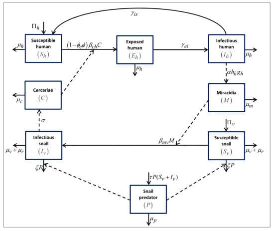
Figure 1. Compartment diagram.

Table 1. Description of model parameters.

Parameter	Description
${\Pi }_h$	Recruitment rate of humans
${\varphi }_e$	Effectiveness of education in reducing contact between humans and cercariae
$\varphi$	Education coverage
${\beta }_{ch}$	Cercaria infection rate on susceptible humans
${\gamma }_{is}$	Recovery rate of infectious humans
${\mu }_h$	Natural death rate of humans
$1/{\gamma }_{ei}$	Latent period
${\Pi }_v$	Recruitment rate of snails
${\beta }_{mv}$	Miracidia infection rate on susceptible snails
${\mu }_v$	Natural death rate of snails
${\mu }_r$	Molluscicide-related death rate of snails
$\xi$	Predation rate
$\tau$	Conversion rate
$\sigma$	Cercaria production rate
$\alpha$	Parasite-egg hatch rate
$h_h$	Number of eggs per gram of stool
$g_h$	Average weight of human stool per day
${\mu }_p$	Natural death rate of snail predators
${\mu }_c$	Natural death rate of cercariae
${\mu }_m$	Natural death rate of miracidiae

On the basis of Figure 1, we constructed a schistosomiasis model as follows:

$$\begin{array}{c}\frac{d{S}_h}{dt}={\Pi }_h-(1-{\varphi }_e\varphi ){\beta }_{ch}C{S}_h+{\gamma }_{is}{I}_h-{\mu }_h{S}_h,\hfill \\ \frac{d{E}_h}{dt}=(1-{\varphi }_e\varphi ){\beta }_{ch}C{S}_h-\left({\gamma }_{ei}+{\mu }_h\right)E_h,\hfill \\ \frac{d{I}_h}{dt}={\gamma }_{ei}{E}_h-\left({\gamma }_{is}+{\mu }_h\right)I_h,\hfill \\ \frac{d{S}_v}{dt}={\Pi }_v-{\beta }_{mv}M{S}_v-({\mu }_v+{\mu }_r)S_v-\xi P{S}_v,\hfill \\ \frac{d{I}_v}{dt}={\beta }_{mv}M{S}_v-({\mu }_v+{\mu }_r)I_v-\xi P{I}_v,\hfill \\ \frac{dC}{dt}=\sigma I_v-{\mu }_{c}C,\hfill \\ \frac{dM}{dt}=\alpha h_h{g}_h{I}_h-{\mu }_{m}M,\hfill \\ \frac{dP}{dt}=\tau P(S_v+I_v)-{\mu }_{p}P,\hfill \end{array}$$

(2)

where $\varphi \in [0,1)$, ${\varphi }_e\in [0,1)$ and the other parameters are positive.

3.2. Invariant Region

In this subsection, we prove that the solutions of System (2) with non-negative initial value are non-negative and bounded.

Theorem 2.

Solutions of System (2) are non-negative for all non-negative initial conditions.

Proof. 

We prove this theorem by using a similar method as that used in [18,23]. From System (2), we have

$$\begin{array}{ccc}\hfill {\left.\frac{d{S}_h}{dt}\right|}_{S_h=0,E_h\ge 0,I_h\ge 0,S_v\ge 0,I_v\ge 0,C\ge 0,M\ge 0,P\ge 0}& =& {\Pi }_h+{\gamma }_{is}{I}_h>0,\hfill \\ \hfill {\left.\frac{d{E}_h}{dt}\right|}_{E_h=0,S_h\ge 0,I_h\ge 0,S_v\ge 0,I_v\ge 0,C\ge 0,M\ge 0,P\ge 0}& =& (1-{\varphi }_e\varphi ){\beta }_{ch}C{S}_h\ge 0,\hfill \\ \hfill {\left.\frac{d{I}_h}{dt}\right|}_{I_h=0,S_h\ge 0,E_h\ge 0,S_v\ge 0,I_v\ge 0,C\ge 0,M\ge 0,P\ge 0}& =& {\gamma }_{ei}{E}_h\ge 0,\hfill \\ \hfill {\left.\frac{d{S}_v}{dt}\right|}_{S_v=0,S_h\ge 0,E_h\ge 0,I_h\ge 0,I_v\ge 0,C\ge 0,M\ge 0,P\ge 0}& =& {\Pi }_v>0,\hfill \\ \hfill {\left.\frac{d{I}_v}{dt}\right|}_{I_v=0,S_h\ge 0,E_h\ge 0,I_h\ge 0,S_v\ge 0,C\ge 0,M\ge 0,P\ge 0}& =& {\beta }_{mv}M{S}_v\ge 0,\hfill \\ \hfill {\left.\frac{dC}{dt}\right|}_{C=0,S_h\ge 0,E_h\ge 0,I_h\ge 0,S_v\ge 0,I_v\ge 0,M\ge 0,P\ge 0}& =& \sigma I_v\ge 0,\hfill \\ \hfill {\left.\frac{dM}{dt}\right|}_{M=0,S_h\ge 0,E_h\ge 0,I_h\ge 0,S_v\ge 0,I_v\ge 0,C\ge 0,P\ge 0}& =& \alpha h_h{g}_h{I}_h\ge 0,\hfill \\ \hfill {\left.\frac{dP}{dt}\right|}_{P=0,S_h\ge 0,E_h\ge 0,I_h\ge 0,S_v\ge 0,I_v\ge 0,C\ge 0,M\ge 0}& =& 0.\hfill \end{array}$$

On the basis of Lemma 2 in [24], ${\mathbb{R}}_{+0}^8$ is an invariant region of System (2). Hence, the solutions of System (2) with initial values in ${\mathbb{R}}_{+0}^8$ remain in ${\mathbb{R}}_{+0}^8$. This completes the proof. □

Theorem 3.

Solutions of System (2) with non-negative initial value are bounded.

Proof. 

On the basis of the assumptions that are used when formulating the model, we have $N_h=S_h+E_h+I_h$ and $N_v=S_v+I_v$. Here, $N_h$ and $N_v$ are the total number of humans and total number of snails, respectively. On the basis of System (2), we have

$$\begin{array}{ccc}\hfill \frac{d{N}_h}{dt}& =& {\Pi }_h-{\mu }_h{N}_h,\hfill \\ \hfill \frac{d{N}_v}{dt}& =& {\Pi }_v-({\mu }_v+{\mu }_r)N_v-\xi P{N}_v,\hfill \\ \hfill \frac{dP}{dt}& =& \tau N_{v}P-{\mu }_{p}P.\hfill \end{array}$$

(3)

First, we prove that $N_h$ is bounded. It is clear that the solution of $\frac{d{N}_h}{dt}={\Pi }_h-{\mu }_h{N}_h$ is

$$N_h\left(t\right)=\frac{{\Pi }_h}{{\mu }_h}+\left(N_h\left(0\right)-\frac{{\Pi }_h}{{\mu }_h}\right)e^{-{\mu }_{h}t}.$$

It easy to see that $0\le N_h\left(t\right)\le \frac{{\Pi }_h}{{\mu }_h}$ for $t\ge 0$ if $0\le N_h\left(0\right)\le \frac{{\Pi }_h}{{\mu }_h}$. Hence, $N_h$ is bounded. $\underset{t\to \infty }{lim}{N}_h\left(t\right)=\frac{{\Pi }_h}{{\mu }_h}$. Now, let $W=N_v+P$. We prove that W is bounded. The last two equations of (3) give

$$\begin{array}{ccc}\hfill \frac{dW}{dt}& =& \frac{d{N}_v}{dt}+\frac{dP}{dt}\hfill \\ \hfill & =& \left({\Pi }_v-({\mu }_v+{\mu }_r)N_v-\xi P{N}_v\right)+\left(\tau N_{v}P-{\mu }_{p}P\right)\hfill \\ \hfill & \le & {\Pi }_v-(\xi -\tau )P{N}_v-\mu (N_v+P)\hfill \\ \hfill & \le & {\Pi }_v-\mu W,\hfill \end{array}$$

(4)

where $\xi \ge \tau$ and $\mu =min\{({\mu }_v+{\mu }_r),{\mu }_p\}$. On the basis of Gronwall’s lemma, we obtain $W=N_v+P\le \frac{{\Pi }_v}{\mu }$. Thus, $N_v$ and P are bounded. Now, we can show that C and M are bounded. We proved that $N_h\le \frac{{\Pi }_h}{{\mu }_h}$, which implies that $I_h\le \frac{{\Pi }_h}{{\mu }_h}$. Moreover, we have $N_v+P\le \frac{{\Pi }_v}{\mu }$, which means that $I_v\le \frac{{\Pi }_v}{\mu }$. Hence, from System (2), we have

$$\begin{array}{ccc}\hfill \frac{dC}{dt}& =& \sigma I_v-{\mu }_{c}C\hfill \\ \hfill & \le & \sigma \frac{{\Pi }_v}{\mu }-{\mu }_{c}C,\hfill \\ \hfill \frac{dM}{dt}& =& \alpha h_h{g}_h{I}_h-{\mu }_{m}M\hfill \\ \hfill & \le & \alpha h_h{g}_h\frac{{\Pi }_h}{{\mu }_h}-{\mu }_{m}M.\hfill \end{array}$$

(5)

According to Gronwall’s lemma, we obtain $C\le \frac{\sigma {\Pi }_v}{\mu {\mu }_c}$ and $M\le \frac{\alpha h_h{g}_h{\Pi }_h}{{\mu }_h{\mu }_m}$. Thus, the solutions of System (2) are bounded. □

Therefore, System (2) is well-posed with invariant region ${\Theta }_{+}$

$$\begin{array}{ccc}\hfill {\Theta }_{+}& =& \{(S_h,E_h,I_h,S_v,I_v,C,M,P)\in {\mathbb{R}}_{+0}^8:N_h\le \frac{{\Pi }_h}{{\mu }_h};N_v+P\le \frac{{\Pi }_v}{\mu };C\le \frac{\sigma {\Pi }_v}{\mu {\mu }_c};M\le \frac{\alpha h_h{g}_h{\Pi }_h}{{\mu }_h{\mu }_m}\}\hfill \end{array}$$

3.3. Equilibrium Points and Basic Reproduction Number

System (2) has four equilibrium points.

• Disease-free equilibrium point $E_0^a$.

  $$E_0^a=(S_h^{a*},E_h^{a*},I_h^{a*},S_v^{a*},I_v^{a*},C^{a*},M^{a*},P^{a*})=\left(\frac{{\Pi }_h}{{\mu }_h},0,0,\frac{{\Pi }_v}{{\mu }_v+{\mu }_r},0,0,0,0\right).$$
  $E_0^a$ always exists in ${\mathbb{R}}_{+0}^8$.
• Endemic equilibrium point $E_1^a$.

  $$E_1^a=(S_h^{a**},E_h^{a**},I_h^{a**},S_v^{a**},I_v^{a**},C^{a**},M^{a**},0),$$

  where

  $$\begin{array}{ccc}\hfill S_h^{a**}& =& \frac{{\Pi }_h({\mu }_h+{\gamma }_{is})({\mu }_h+{\gamma }_{ei}){\mu }_c}{(({\mu }_h+{\gamma }_{ei})({\mu }_h+{\gamma }_{is})-{\gamma }_{ei}{\gamma }_{is})(1-{\varphi }_e\varphi ){\beta }_{ch}\sigma I_v^{a**}+{\mu }_h({\mu }_h+{\gamma }_{is})({\mu }_h+{\gamma }_{ei}){\mu }_c},\hfill \\ \hfill \\ \hfill E_h^{a**}& =& \frac{{\Pi }_h({\mu }_h+{\gamma }_{is})(1-{\varphi }_e\varphi ){\beta }_{ch}\sigma I_v^{a**}}{(({\mu }_h+{\gamma }_{ei})({\mu }_h+{\gamma }_{is})-{\gamma }_{ei}{\gamma }_{is})(1-{\varphi }_e\varphi ){\beta }_{ch}\sigma I_v^{a**}+{\mu }_h({\mu }_h+{\gamma }_{is})({\mu }_h+{\gamma }_{ei}){\mu }_c},\hfill \\ \hfill \\ \hfill I_h^{a**}& =& \frac{{\Pi }_h{\gamma }_{ei}(1-{\varphi }_e\varphi ){\beta }_{ch}\sigma I_v^{a**}}{(({\mu }_h+{\gamma }_{ei})({\mu }_h+{\gamma }_{is})-{\gamma }_{ei}{\gamma }_{is})(1-{\varphi }_e\varphi ){\beta }_{ch}\sigma I_v^{a**}+{\mu }_h({\mu }_h+{\gamma }_{is})({\mu }_h+{\gamma }_{ei}){\mu }_c},\hfill \\ \hfill \\ \hfill S_v^{a**}& =& \frac{{\Pi }_v}{{\mu }_v+{\mu }_r}-I_v^{a**},\hfill \\ \hfill \\ \hfill I_v^{a**}& =& \frac{(R_e^a-1){\mu }_h({\mu }_h+{\gamma }_{ei})({\mu }_h+{\gamma }_{is}){\mu }_c{\mu }_m({\mu }_v+{\mu }_r)}{{\beta }_{mv}{\Pi }_h{\gamma }_{ei}(1-{\varphi }_e\varphi )\alpha h_h{g}_h{\beta }_{ch}\sigma +(({\mu }_h+{\gamma }_{ei})({\mu }_h+{\gamma }_{is})-{\gamma }_{ei}{\gamma }_{is}){\mu }_m(1-{\varphi }_e\varphi ){\beta }_{ch}\sigma ({\mu }_v+{\mu }_r)},\hfill \\ \hfill \\ \hfill C^{a**}& =& \frac{\sigma I_v^{a**}}{{\mu }_c},\hfill \\ \hfill \\ \hfill M^{a**}& =& \frac{\alpha h_h{g}_h{\Pi }_h{\gamma }_{ei}(1-{\varphi }_e\varphi ){\beta }_{ch}\sigma I_v^{a**}}{{\mu }_m((({\mu }_h+{\gamma }_{ei})({\mu }_h+{\gamma }_{is})-{\gamma }_{ei}{\gamma }_{is})(1-{\varphi }_e\varphi ){\beta }_{ch}\sigma I_v^{a**}+{\mu }_h({\mu }_h+{\gamma }_{is})({\mu }_h+{\gamma }_{ei}){\mu }_c)},\hfill \\ \hfill \\ \hfill R_e^a& =& \frac{{\Pi }_h{\Pi }_v{\gamma }_{ei}(1-{\varphi }_e\varphi ){\beta }_{ch}\sigma \alpha h_h{g}_h{\beta }_{mv}}{{\mu }_h({\mu }_h+{\gamma }_{ei})({\mu }_h+{\gamma }_{is}){\mu }_c{\mu }_m{({\mu }_v+{\mu }_r)}^2}.\hfill \end{array}$$
  It is clear that $E_1^a$ exists in ${\mathbb{R}}_{+0}^8$ if $R_e^a>1$.
• Disease-free equilibrium point $E_0^b$.

  $$E_0^b=(S_h^{b*},E_h^{b*},I_h^{b*},S_v^{b*},I_v^{b*},C^{b*},M^{b*},P^{b*})=\left(\frac{{\Pi }_h}{{\mu }_h},0,0,\frac{{\mu }_p}{\tau },0,0,0,\frac{{\Pi }_v\tau -({\mu }_v+{\mu }_r){\mu }_p}{\xi {\mu }_p}\right),$$
  $E_0^b$ exists in ${\mathbb{R}}_{+0}^8$ if $\frac{{\Pi }_v\tau }{({\mu }_v+{\mu }_r){\mu }_p}>1$.
• Endemic equilibrium point $E_1^b$.

  $$E_1^b=(S_h^{b**},E_h^{b**},I_h^{b**},S_v^{b**},I_v^{b**},C^{b**},M^{b**},P^{b**}),$$

  where

  $$\begin{array}{ccc}\hfill S_h^{b**}& =& \frac{{\Pi }_h({\mu }_h+{\gamma }_{is})({\mu }_h+{\gamma }_{ei}){\mu }_c}{(({\mu }_h+{\gamma }_{ei})({\mu }_h+{\gamma }_{is})-{\gamma }_{ei}{\gamma }_{is})(1-{\varphi }_e\varphi ){\beta }_{ch}\sigma I_v^{b**}+{\mu }_h({\mu }_h+{\gamma }_{is})({\mu }_h+{\gamma }_{ei}){\mu }_c},\hfill \\ \hfill \\ \hfill E_h^{b**}& =& \frac{{\Pi }_h({\mu }_h+{\gamma }_{is})(1-{\varphi }_e\varphi ){\beta }_{ch}\sigma I_v^{b**}}{(({\mu }_h+{\gamma }_{ei})({\mu }_h+{\gamma }_{is})-{\gamma }_{ei}{\gamma }_{is})(1-{\varphi }_e\varphi ){\beta }_{ch}\sigma I_v^{b**}+{\mu }_h({\mu }_h+{\gamma }_{is})({\mu }_h+{\gamma }_{ei}){\mu }_c},\hfill \\ \hfill \\ \hfill I_h^{b**}& =& \frac{{\Pi }_h{\gamma }_{ei}(1-{\varphi }_e\varphi ){\beta }_{ch}\sigma I_v^{b**}}{(({\mu }_h+{\gamma }_{ei})({\mu }_h+{\gamma }_{is})-{\gamma }_{ei}{\gamma }_{is})(1-{\varphi }_e\varphi ){\beta }_{ch}\sigma I_v^{b**}+{\mu }_h({\mu }_h+{\gamma }_{is})({\mu }_h+{\gamma }_{ei}){\mu }_c},\hfill \\ \hfill \\ \hfill S_v^{b**}& =& \frac{{\mu }_p}{\tau }-I_v^{b**},\hfill \\ \hfill \\ \hfill I_v^{b**}& =& \frac{(R_e^b-1){\mu }_h({\mu }_h+{\gamma }_{ei})({\mu }_h+{\gamma }_{is}){\mu }_c{\mu }_m(({\mu }_v+{\mu }_r)+\xi P^{b**})}{{\beta }_{mv}{\Pi }_h{\gamma }_{ei}(1-{\varphi }_e\varphi )\alpha h_h{g}_h{\beta }_{ch}\sigma +(({\mu }_h+{\gamma }_{ei})({\mu }_h+{\gamma }_{is})-{\gamma }_{ei}{\gamma }_{is}){\mu }_m(1-{\varphi }_e\varphi ){\beta }_{ch}\sigma (({\mu }_v+{\mu }_r)+\xi P^{b**})},\hfill \\ \hfill \\ \hfill C^{b**}& =& \frac{\sigma I_v^{b**}}{{\mu }_c},\hfill \\ \hfill \\ \hfill M^{b**}& =& \frac{\alpha h_h{g}_h{\Pi }_h{\gamma }_{ei}(1-{\varphi }_e\varphi ){\beta }_{ch}\sigma I_v^{b**}}{{\mu }_m((({\mu }_h+{\gamma }_{ei})({\mu }_h+{\gamma }_{is})-{\gamma }_{ei}{\gamma }_{is})(1-{\varphi }_e\varphi ){\beta }_{ch}\sigma I_v^{b**}+{\mu }_h({\mu }_h+{\gamma }_{is})({\mu }_h+{\gamma }_{ei}){\mu }_c)},\hfill \\ \hfill \\ \hfill P^{b**}& =& \frac{{\Pi }_v\tau -({\mu }_v+{\mu }_r){\mu }_p}{\xi {\mu }_p}\hfill \\ \hfill \\ \hfill R_e^b& =& \frac{{\Pi }_h{\mu }_p{\gamma }_{ei}(1-{\varphi }_e\varphi ){\beta }_{ch}\sigma \alpha h_h{g}_h{\beta }_{mv}}{{\mu }_h({\mu }_h+{\gamma }_{ei})({\mu }_h+{\gamma }_{is}){\mu }_c{\mu }_m\tau ({\mu }_v+{\mu }_r+\xi P^{b**})}.\hfill \end{array}$$
  It is clear that $E_1^b$ exists in ${\mathbb{R}}_{+0}^8$ if $R_e^b>1$ and $\frac{{\Pi }_v\tau }{({\mu }_v+{\mu }_r){\mu }_p}>1$.

The basic reproduction numbers are determined by using a next-generation matrix [25]. Here, we regard $E_h$, $I_h$, $I_v$, C, and M as the infected compartments. Thus, we have

$$\begin{array}{ccc}\mathcal{F}=\left(\begin{array}{c}(1-{\varphi }_e\varphi ){\beta }_{ch}C{S}_h\\ 0\\ {\beta }_{mv}M{S}_v\\ 0\\ 0\end{array}\right)\hfill & ,& \mathcal{V}=\left(\begin{array}{c}({\gamma }_{ei}+{\mu }_h)E_h\\ ({\gamma }_{is}+{\mu }_h)I_h-{\gamma }_{ei}{E}_h\\ ({\mu }_v+{\mu }_r+\xi P)I_v\\ {\mu }_{c}C-\sigma I_v\\ {\mu }_{m}M-\alpha h_h{g}_h{I}_h\end{array}\right).\hfill \end{array}$$

$\mathcal{F}$ and $\mathcal{V}$ represent the new infection terms and transition terms, respectively. The Jacobian matrices of $\mathcal{F}$ and $\mathcal{V}$ at arbitrary equilibrium point $(S_h^{*},0,0,S_v^{*},0,0,0,P^{*})$ are, respectively, given by

$$F=\left(\begin{array}{ccccc}0& 0& 0& {\beta }_{ch}(1-{\varphi }_e\varphi )S_h^{*}& 0\\ 0& 0& 0& 0& 0\\ 0& 0& 0& 0& {\beta }_{mv}{S}_v^{*}\\ 0& 0& 0& 0& 0\\ 0& 0& 0& 0& 0\end{array}\right),$$

and

$$V=\left(\begin{array}{ccccc}{\mu }_h+{\gamma }_{ei}& 0& 0& 0& 0\\ -{\gamma }_{ei}& {\mu }_h+{\gamma }_{is}& 0& 0& 0\\ 0& 0& {\mu }_v+{\mu }_r+\xi P^{*}& 0& 0\\ 0& 0& -\sigma & {\mu }_c& 0\\ 0& -\alpha h_h{g}_h& 0& 0& {\mu }_m\end{array}\right).$$

The basic reproduction number is the spectral radius of $F{V}^{-1}$.

$$\begin{array}{ccc}\hfill F{V}^{-1}& =& \left(\begin{array}{ccccc}0& 0& \frac{{\beta }_{ch}(1-{\varphi }_e\varphi )S_h^{*}\sigma }{{\mu }_c(({\mu }_v+{\mu }_r)+\xi P^{*})}& \frac{{\beta }_{ch}(1-{\varphi }_e\varphi )S_h^{*}}{{\mu }_c}& 0\\ 0& 0& 0& 0& 0\\ \frac{{\beta }_{mv}{S}_v^{*}\alpha h_h{g}_h{\gamma }_{ei}}{({\mu }_h+{\gamma }_{ei})({\mu }_h+{\gamma }_{is}){\mu }_m}& \frac{{\beta }_{mv}{S}_v^{*}\alpha h_h{g}_h}{({\mu }_h+{\gamma }_{is}){\mu }_m}& 0& 0& \frac{{\beta }_{mv}{S}_v^{*}}{{\mu }_m}\\ 0& 0& 0& 0& 0\\ 0& 0& 0& 0& 0\end{array}\right).\hfill \end{array}$$

(6)

The characteristic polynomial of (6) is

$$\mathbf{P}\left(\lambda \right)={\lambda }^3\left({\lambda }^2-\frac{(1-{\varphi }_e\varphi ){\beta }_{ch}{S}_h^{*}\sigma {\beta }_{mv}{\S }_v^{*}\alpha h_h{g}_h{\gamma }_{ei}}{(({\mu }_v+{\mu }_r)+\xi P^{*}){\mu }_c{\mu }_m({\mu }_h+{\gamma }_{ei})({\mu }_h+{\gamma }_{is})}\right).$$

Thus, the spectral radius of $F{V}^{-1}$ is

$$\rho \left(F{V}^{-1}\right)=\sqrt{\frac{(1-{\varphi }_e\varphi ){\beta }_{ch}{S}_h^{*}\sigma {\beta }_{mv}{S}_v^{*}\alpha h_h{g}_h{\gamma }_{ei}}{(({\mu }_v+{\mu }_r)+\xi P^{*}){\mu }_c{\mu }_m({\mu }_h+{\gamma }_{ei})({\mu }_h+{\gamma }_{is})}}.$$

(7)

By substituting $E_0^a$ into (7), we obtain the basic reproduction number when the predator becomes extinct.

$$R_0^a=\sqrt{\frac{(1-{\varphi }_e\varphi ){\beta }_{ch}{\Pi }_h\sigma {\beta }_{mv}{\Pi }_v\alpha h_h{g}_h{\gamma }_{ei}}{{\mu }_h{({\mu }_v+{\mu }_r)}^2{\mu }_c{\mu }_m({\mu }_h+{\gamma }_{ei})({\mu }_h+{\gamma }_{is})}}.$$

$R_0^a>0$ and $R_e^a={\left(R_0^a\right)}^2$. In agreement with the existence condition of $E_1^a$, if $R_0^a>1$ then $E_1^a$ exists in ${\mathbb{R}}_{+0}^8$. It is easy to see that $R_0^a$ is completely independent from parameters that are related to the snail predator. This makes sense because $E_0^a$ and $E_1^a$ describe the condition when the predator becomes extinct.

After substituting $E_0^b$ into (7), we obtain the basic reproduction number when the predator survives, namely,

$$\begin{array}{ccc}\hfill R_0^b& =& \sqrt{\frac{(1-{\varphi }_e\varphi ){\beta }_{ch}{\Pi }_h\sigma {\beta }_{mv}{\mu }_p\alpha h_h{g}_h{\gamma }_{ei}}{{\mu }_h(({\mu }_v+{\mu }_r)+\xi P^{b*}){\mu }_c{\mu }_m({\mu }_h+{\gamma }_{ei})({\mu }_h+{\gamma }_{is})\tau }}\hfill \\ \hfill & & \hfill \\ \hfill & =& \sqrt{\frac{(1-{\varphi }_e\varphi ){\beta }_{ch}{\Pi }_h\sigma {\beta }_{mv}{\mu }_p\alpha h_h{g}_h{\gamma }_{ei}}{{\mu }_h\left(({\mu }_v+{\mu }_r)+\xi \left(\frac{{\Pi }_v\tau -({\mu }_v+{\mu }_r){\mu }_p}{\xi {\mu }_p}\right)\right){\mu }_c{\mu }_m({\mu }_h+{\gamma }_{ei})({\mu }_h+{\gamma }_{is})\tau }}\hfill \\ \hfill & & \hfill \\ \hfill & =& \sqrt{\frac{(1-{\varphi }_e\varphi ){\beta }_{ch}{\Pi }_h\sigma {\beta }_{mv}{\mu }_p^2\alpha h_h{g}_h{\gamma }_{ei}}{{\mu }_h{\Pi }_v{\mu }_c{\mu }_m({\mu }_h+{\gamma }_{ei})({\mu }_h+{\gamma }_{is}){\tau }^2}}.\hfill \end{array}$$

$R_0^b>0$ and $R_e^b={\left(R_0^b\right)}^2$. In line with the existence condition of $E_1^b$, if $R_0^b>1$ and $\frac{{\Pi }_v\tau }{({\mu }_v+{\mu }_r){\mu }_p}>1$, then $E_1^b$ exists in ${\mathbb{R}}_{+0}^8$. $R_0^b$ is independent to $\xi$. Furthermore, it is clear that $R_0^b$ decreases as $\tau$ increases. The higher the natural death rate of the snail predator is, the higher $R_0^b$ is.

4. Stability Analysis

In this section, we investigate the stability condition of all equilibrium points. The Jacobian matrix of System (2) at $E_0^a$ is

$$J\left(E_0^a\right)=\left(\begin{array}{cccccccc}-{\mu }_h& 0& {\gamma }_{is}& 0& 0& -(1-{\varphi }_e\varphi ){\beta }_{ch}{S}_h^{a*}& 0& 0\\ 0& -({\gamma }_{ei}+{\mu }_h)& 0& 0& 0& (1-{\varphi }_e\varphi ){\beta }_{ch}{S}_h^{a*}& 0& 0\\ 0& {\gamma }_{ei}& -({\gamma }_{is}+{\mu }_h)& 0& 0& 0& 0& 0\\ 0& 0& 0& -({\mu }_v+{\mu }_r)& 0& 0& -{\beta }_{mv}{S}_v^{a*}& -\xi S_v^{a*}\\ 0& 0& 0& 0& -({\mu }_v+{\mu }_r)& 0& {\beta }_{mv}{S}_v^{a*}& 0\\ 0& 0& 0& 0& \sigma & -{\mu }_c& 0& 0\\ 0& 0& \alpha h_h{g}_h& 0& 0& 0& -{\mu }_m& 0\\ 0& 0& 0& 0& 0& 0& 0& \tau S_v^{a*}-{\mu }_p\end{array}\right)$$

(8)

The eigenvalues of (8) are zeroes of $L\left(\lambda \right)$

$$\begin{array}{ccc}\hfill L\left(\lambda \right)& =& \left[(\lambda +D_1)(\lambda +D_2)(\lambda +D_3)(\lambda +D_4)(\lambda +D_5)-{\gamma }_{ei}\alpha h_h{g}_h(1-{\varphi }_e\varphi ){\beta }_{ch}{S}_h^{a*}\sigma {\beta }_{mv}{S}_v^{a*}\right]\hfill \\ \hfill & & \times (\lambda +{\mu }_h)(\lambda +({\mu }_v+{\mu }_r))(\lambda -(\tau S_v^{a*}-{\mu }_p))\hfill \\ \hfill & =& \left[L_1\left(\lambda \right)\right](\lambda +{\mu }_h)(\lambda +({\mu }_v+{\mu }_r))(\lambda -(\tau S_v^{a*}-{\mu }_p)),\hfill \end{array}$$

(9)

where

$$\begin{array}{ccc}\hfill L_1\left(\lambda \right)& =& {\lambda }^5+l_1{\lambda }^4+l_2{\lambda }^3+l_3{\lambda }^2+l_4\lambda +l_5,\hfill \\ \hfill l_1& =& {\displaystyle \sum _{g=1}^5}{D}_g,\hfill \\ \hfill l_2& =& {\displaystyle \sum _{1\le g<h}^5}{D}_g{D}_h,\hfill \\ \hfill l_3& =& {\displaystyle \sum _{1\le g<h<i}^5}{D}_g{D}_h{D}_i,\hfill \\ \hfill l_4& =& {\displaystyle \sum _{1\le g<\dots <j}^5}{D}_g{D}_h{D}_i{D}_j,\hfill \\ \hfill l_5& =& ({\mu }_h+{\gamma }_{ei})({\mu }_h+{\gamma }_{is})({\mu }_v+{\mu }_r){\mu }_c{\mu }_m-{\gamma }_{ei}\alpha h_h{g}_h(1-{\varphi }_e\varphi ){\beta }_{ch}{S}_h^{a*}\sigma {\beta }_{mv}{S}_v^{a*}\hfill \\ \hfill & =& \left(1-{\left(R_0^a\right)}^2\right)({\mu }_h+{\gamma }_{ei})({\mu }_h+{\gamma }_{is})({\mu }_v+{\mu }_r){\mu }_c{\mu }_m,\hfill \end{array}$$

(10)

$D_1={\mu }_h+{\gamma }_{ei}>0,D_2={\mu }_h+{\gamma }_{is}>0,D_3={\mu }_v+{\mu }_r>0,D_4={\mu }_c>0,$ and $D_5={\mu }_m>0$. Clearly, $l_i$ for $i=1,2,3,4,5$ are elementary symmetric functions [26]. It is obvious that (8) has two negative eigenvalues, i.e., ${\lambda }_1=-{\mu }_h$ and ${\lambda }_2=-({\mu }_v+{\mu }_r)$. Moreover, ${\lambda }_3=\tau S_v^{a*}-{\mu }_p<0$ if $\frac{\tau S_v^{a*}}{{\mu }_p}=\frac{\tau {\Pi }_v}{{\mu }_p({\mu }_v+{\mu }_r)}<1$. The other eigenvalues are zeroes of $L_1\left(\lambda \right)$. It is easy to see that $l_i>0$ for $i=1,2,\dots ,5$ if $R_0^a<1$. If $R_0^a=1$ then $l_5=0$. Hence, if $\frac{\tau S_v^{a*}}{{\mu }_p}=\frac{\tau {\Pi }_v}{{\mu }_p({\mu }_v+{\mu }_r)}<1$ and $R_0^a=1$ then one eigenvalue of $J\left(E_0^a\right)$ is zero. Following [27,28], we use a Routh–Hurwitz array shown in Table 2 to determine the Hurwitz determinant.

Table 2. Routh–Hurwitz array associated with characteristic polynomial $L_1\left(\lambda \right)$.

	Column 1	Column 2	Column 3	Column 4
${\lambda }^5$	1	$l_2$	$l_4$	0
${\lambda }^4$	${\Delta }_1=l_1$	$l_3$	$l_5$	0
${\lambda }^3$	$r_{(2,1)}=\frac{l_1{l}_2-l_3}{l_1}$	$r_{(2,2)}=\frac{l_1{l}_4-l_5}{l_1}$	0	0
${\lambda }^2$	$r_{(3,1)}=\frac{r_{(2,1)}{l}_3-l_1{r}_{(2,2)}}{r_{(2,1)}}$	$l_5$	0	0
${\lambda }^1$	$r_{(4,1)}=\frac{r_{(2,2)}{r}_{(3,1)}-l_5{r}_{(2,1)}}{r_{(3,1)}}$	0	0	0
${\lambda }^0$	$r_{(5,1)}=l_5$	0	0	0

The Hurwitz determinant of order-i$\left({\Delta }_i\right)$ is given by ${\Delta }_i=r_{(i,1)}{\Delta }_{i-1}$ for $i=2,3,4,5$. Hence we obtain

$$\begin{array}{ccc}\hfill {\Delta }_1& =& l_1,\hfill \\ \hfill {\Delta }_2& =& \left(\frac{l_1{l}_2-l_3}{l_1}\right){\Delta }_1\hfill \\ \hfill & =& l_1{l}_2-l_3,\hfill \\ \hfill {\Delta }_3& =& \left(\frac{l_3(l_1{l}_2-l_3)-l_1(l_1{l}_4-l_5)}{l_1{l}_2-l_3}\right){\Delta }_2\hfill \\ \hfill & =& l_3(l_1{l}_2-l_3)-l_1(l_1{l}_4-l_5),\hfill \end{array}$$

$$\begin{array}{ccc}\hfill {\Delta }_4& =& \left(\frac{l_4\left[(l_1{l}_2-l_3)l_3-l_1(l_1{l}_4-l_5)\right]-l_5\left[l_2(l_2{l}_1-l_3)-(l_1{l}_4-l_5)\right]}{l_3(l_1{l}_2-l_3)-l_1(l_1{l}_4-l_5)}\right){\Delta }_3\hfill \\ \hfill & =& l_4\left[(l_1{l}_2-l_3)l_3-l_1(l_1{l}_4-l_5)\right]-l_5\left[l_2(l_2{l}_1-l_3)-(l_1{l}_4-l_5)\right],\hfill \\ \hfill {\Delta }_5& =& l_5{\Delta }_4\hfill \\ \hfill & =& l_5\left(l_4\left[(l_1{l}_2-l_3)l_3-l_1(l_1{l}_4-l_5)\right]-l_5\left[l_2(l_2{l}_1-l_3)-(l_1{l}_4-l_5)\right]\right).\hfill \end{array}$$

We prove this theorem by using the Liénard–Chipart criterion [29]. According to the criterion, all roots of $L_1\left(\lambda \right)$ have a negative real part if $l_1,{\Delta }_2,l_3,{\Delta }_4,l_5>0$. It is clear that $l_i>0$ always holds for $i=1,3$. Furthermore, $l_5>0$ if $R_0^a<1$. Now, we only need to check ${\Delta }_2$ and ${\Delta }_4$. First, we set

$$R_0^a=\sqrt{\frac{R_{01}^a}{R_{02}^a}},$$

where

$$\begin{array}{ccc}\hfill R_{01}^a& =& {\gamma }_{ei}\alpha h_h{g}_h(1-{\varphi }_e\varphi ){\beta }_{ch}{S}_h^{a*}\sigma {\beta }_{mv}{S}_v^{a*}\hfill \\ \hfill R_{02}^a& =& D_1{D}_2{D}_3{D}_4{D}_5.\hfill \end{array}$$

It is clear that $R_{01}^a>0$ and $R_{02}^a>0$. Therefore, $R_0^a<1$ implies $R_{01}^a<R_{02}^a$. We now investigate ${\Delta }_2$ and ${\Delta }_4$.

$$\begin{array}{ccc}\hfill {\Delta }_2& =& l_1{l}_2-l_3\hfill \\ \hfill & =& D_1(D_2+D_3+D_4+D_5)(D_1+D_2+D_3+D_4+D_5)\hfill \\ \hfill & & +D_2(D_2+D_3+D_4+D_5)(D_3+D_4+D_5)\hfill \\ \hfill & & +(D_3+D_4+D_5)(D_4+D_5)+D_4(D_4{D}_5+D_5{D}_5),\hfill \\ \hfill {\Delta }_4& =& l_4\left[(l_1{l}_2-l_3)l_3-l_1(l_1{l}_4-l_5)\right]-l_5\left[l_2(l_2{l}_1-l_3)-(l_1{l}_4-l_5)\right]\hfill \\ \hfill & =& \Xi +12R_{01}^a{R}_{02}^a-R_{01}^a{R}_{01}^a\hfill \\ \hfill & =& \Xi +R_{01}^{a}12R_{02}^a-R_{01}^a{R}_{01}^a\hfill \\ \hfill & =& \Xi +R_{01}^a\left(12R_{02}^a-R_{01}^a\right).\hfill \end{array}$$

Since $D_i>0$ for $i=1,2,3,4,5$, it is clear that ${\Delta }_2>0$. We also proved that $\Xi >0$ (see Appendix A). Thus, ${\Delta }_4>0$ if $R_0^a<1$. Therefore, on the basis of the Liénard–Chipart criterion [29], all zeroes of $L_1\left(\lambda \right)$ have a negative real part if $R_0^a<1$. Hence, all eigenvalues of $J\left(E_0^a\right)$ have a negative real part if $R_0^a<1$ and $\frac{\tau {\Pi }_v}{{\mu }_p({\mu }_v+{\mu }_r)}<1$. Therefore, $E_0^a$ is asymptotically stable if $R_0^a<1$ and $\frac{\tau {\Pi }_v}{{\mu }_p({\mu }_v+{\mu }_r)}<1$. If $R_0^a>1$, then there is one sign change in the sequence of $L_1\left(\lambda \right)$ coefficients. On the basis of Descartes’ sign rule [26], there is exactly one positive real root if $R_0^a>1$. Hence, $E_0^a$ is unstable if $R_0^a>1$.

Theorem 4.

Disease-free equilibrium point $E_0^a$ is asymptotically stable if $R_0^a<1$ and $\frac{\tau {\Pi }_v}{{\mu }_p({\mu }_v+{\mu }_r)}<1$. If $R_0^a>1$ or $\frac{\tau {\Pi }_v}{{\mu }_p({\mu }_v+{\mu }_r)}>1$ then $E_0^a$ is unstable.

Now, we present the local stability condition of $E_1^a$.

Theorem 5.

Endemic equilibrium point $E_1^a$ is asymptotically stable if $R_0^a>1$ (near 1) and $\frac{\tau {\Pi }_v}{{\mu }_p({\mu }_v+{\mu }_r)}<1$.

Proof. 

We use Theorem 1 to prove this theorem. Consider ${\beta }_{ch}$ as bifurcation parameter. We determine the bifurcation point when $R_0^a=1$. The bifurcation point that is obtained is ${\beta }_{ch}^{*}=\frac{{\mu }_h{({\mu }_v+{\mu }_r)}^2{\mu }_c{\mu }_m({\mu }_h+{\gamma }_{ei})({\mu }_h+{\gamma }_{is})}{(1-{\varphi }_e\varphi ){\Pi }_h\sigma {\beta }_{mv}{\Pi }_v\alpha h_h{g}_h{\gamma }_{ei}}$. When ${\beta }_{ch}={\beta }_{ch}^{*}$, the characteristic polynomial (9) becomes

$$\begin{array}{ccc}\hfill L\left(\lambda \right)& =& \left[L_1\left(\lambda \right)\right](\lambda +{\mu }_h)(\lambda +({\mu }_v+{\mu }_r))(\lambda -(\tau S_v^{a*}-{\mu }_p))\lambda ,\hfill \end{array}$$

(11)

where

$$\begin{array}{ccc}\hfill L_1\left(\lambda \right)& =& {\lambda }^4+l_1{\lambda }^3+l_2{\lambda }^2+l_3\lambda +l_4.\hfill \end{array}$$

(12)

It is clear that characteristic polynomial (11) has simple zero root $({\lambda }_1=0)$ and two negative roots, i.e., ${\lambda }_2=-{\mu }_h$ and ${\lambda }_3=-({\mu }_v+{\mu }_r)$. Moreover, ${\lambda }_4=\tau S_v^{a*}-{\mu }_p<0$ if $\frac{\tau S_v^{a*}}{{\mu }_p}=\frac{\tau {\Pi }_v}{{\mu }_p({\mu }_v+{\mu }_r)}<1$. Using the Routh–Hurwitz array in Table 3, we determine the conditions that guarantee that the other roots of (11) have a negative real part.

Table 3. Routh–Hurwitz array associated with characteristic polynomial (12).

	Column 1	Column 2	Column 3	Column 4
${\lambda }^4$	1	$l_2$	$l_4$	0
${\lambda }^3$	$l_1$	$l_3$	0	0
${\lambda }^2$	$r_1=\frac{l_1{l}_2-l_3}{l_1}$	$l_4$	0	0
${\lambda }^1$	$r_2=\frac{r_1{l}_3-l_1{l}_4}{r_1}$	0	0	0
${\lambda }^0$	$l_4$	0	0	0

$l_1,r_1,r_2,l_4>0$ (see Appendix B). Hence, on the basis of the Routh–Hurwitz criterion [27], all roots of (12) have a negative real part. These results imply that, if $\frac{\tau {\Pi }_v}{{\mu }_p({\mu }_v+{\mu }_r)}<1$, then $J\left(E_0^a,{\beta }_{ch}^{*}\right)$ has one zero eigenvalue, and the other eigenvalues have a negative real part. Thus, Assumption A1 in Theorem 1 is satisfied if $\frac{\tau {\Pi }_v}{{\mu }_p({\mu }_v+{\mu }_r)}<1$. The right eigenvector of $J\left(E_0^a,{\beta }_{ch}^{*}\right)$ corresponding to a zero eigenvalue is

$$\overrightarrow{v^a}=\left(\begin{array}{c}{v}_1^a\\ v_2^a\\ v_3^a\\ v_4^a\\ v_5^a\\ v_6^a\\ v_7^a\\ v_8^a\end{array}\right)=\left(\begin{array}{c}\frac{({\gamma }_{is}{\gamma }_{ei}-({\mu }_h+{\gamma }_{ei})({\mu }_h+{\gamma }_{is}))(1-{\varphi }_e\varphi ){\beta }_{ch}^{*}{S}_h^{a*}{v}_6^a}{{\mu }_h({\mu }_h+{\gamma }_{ei})({\mu }_h+{\gamma }_{is})}\\ \frac{(1-{\varphi }_e\varphi ){\beta }_{ch}^{*}{S}_h^{a*}{v}_6^a}{{\mu }_h+{\gamma }_{ei}}\\ \frac{{\gamma }_{ei}(1-{\varphi }_e\varphi ){\beta }_{ch}^{*}{S}_h^{a*}{v}_6^a}{({\mu }_h+{\gamma }_{is})({\mu }_h+{\gamma }_{ei})}\\ \frac{-{\beta }_{mv}{S}_v^{a*}\alpha h_h{g}_h{\gamma }_{ei}(1-{\varphi }_e\varphi ){\beta }_{ch}^{*}{S}_h^{a*}{v}_6^a}{({\mu }_h+{\gamma }_{is})({\mu }_h+{\gamma }_{ei})({\mu }_v+{\mu }_r){\mu }_m}\\ \frac{{\beta }_{mv}{S}_v^{a*}\alpha h_h{g}_h{\gamma }_{ei}(1-{\varphi }_e\varphi ){\beta }_{ch}^{*}{S}_h^{a*}{v}_6^a}{({\mu }_h+{\gamma }_{is})({\mu }_h+{\gamma }_{ei})({\mu }_v+{\mu }_r){\mu }_m}\\ v_6^a\\ \frac{\alpha h_h{g}_h{\gamma }_{ei}(1-{\varphi }_e\varphi ){\beta }_{ch}^{*}{S}_h^{a*}{v}_6^a}{({\mu }_h+{\gamma }_{is})({\mu }_h+{\gamma }_{ei}){\mu }_m}\\ 0\end{array}\right),$$

where $v_6^a$ is arbitrarily positive. It is clear that $v_1^a<0$ and $v_4^a<0$. The left eigenvector of $J\left(E_0^a,{\beta }_{ch}^{*}\right)$, corresponding to a zero eigenvalue is

$${\overrightarrow{w^a}}^T=\left(\begin{array}{c}{w}_1^a\\ w_2^a\\ w_3^a\\ w_4\\ w_5^a\\ w_6^a\\ w_7^a\\ w_8^a\end{array}\right)=\left(\begin{array}{c}0\\ \frac{{\gamma }_{ei}\alpha h_h{g}_h\sigma {\beta }_{mv}{S}_v^{a*}{w}_6^a}{({\mu }_h+{\gamma }_{is})({\mu }_h+{\gamma }_{ei})({\mu }_v+{\mu }_r){\mu }_m}\\ \frac{\alpha h_h{g}_h\sigma {\beta }_{mv}{S}_v^{a*}{w}_6^a}{({\mu }_h+{\gamma }_{is})({\mu }_v+{\mu }_r){\mu }_m}\\ 0\\ \frac{\sigma w_6^a}{{\mu }_v+{\mu }_r}\\ w_6^a\\ \frac{{\beta }_{mv}{S}_v^{a*}\sigma w_6^a}{{\mu }_m({\mu }_v+{\mu }_r)}\\ 0\end{array}\right),$$

where $w_6^a$ is determined, such that $\overrightarrow{w^a}.\overrightarrow{v^a}=1$. It is straightforward to show that $w_6^a>0$. Let

$$\begin{array}{ccccccc}{x}_1=S_h& ,& x_2=E_h& ,& x_3=I_h& ,& x_4=S_v,\\ x_5=I_v& ,& x_6=C& ,& x_7=M& ,& x_8=P,\\ f_1=\frac{d{S}_h}{dt}& ,& f_2=\frac{d{E}_h}{dt}& ,& f_3=\frac{d{I}_h}{dt}& ,& f_4=\frac{d{S}_v}{dt},\\ f_5=\frac{d{I}_v}{dt}& ,& f_6=\frac{dC}{dt}& ,& f_7=\frac{dM}{dt}& ,& f_8=\frac{dP}{dt}.\end{array}$$

Now, we compute A and B that are defined in Theorem 1. It is clear that the only nonzero terms of A and B are

$$\begin{array}{cc}\hfill w_2^a{v}_1^a{v}_6^a\frac{{\partial }^2{f}_2\left(E_0^a,{\beta }_{ch}^{*}\right)}{\partial x_1\partial x_6}=& \left(\frac{{\gamma }_{ei}\alpha h_h{g}_h\sigma {\beta }_{mv}{S}_v^{a*}{w}_6^a}{({\mu }_h+{\gamma }_{is})({\mu }_h+{\gamma }_{ei})({\mu }_v+{\mu }_r){\mu }_m}\right)\hfill \\ \hfill & \times \left(\frac{({\gamma }_{is}{\gamma }_{ei}-({\mu }_h+{\gamma }_{ei})({\mu }_h+{\gamma }_{is}))(1-{\varphi }_e\varphi ){\beta }_{ch}^{*}{S}_h^{a*}{v}_6^a}{{\mu }_h({\mu }_h+{\gamma }_{ei})({\mu }_h+{\gamma }_{is})}\right)v_6^a{\beta }_{ch}^{*}<0,\hfill \end{array}$$

$$\begin{array}{cc}\hfill w_2^a{v}_6^a{v}_1^a\frac{{\partial }^2{f}_2\left(E_0^a,{\beta }_{ch}^{*}\right)}{\partial x_6\partial x_1}=& \left(\frac{{\gamma }_{ei}\alpha h_h{g}_h\sigma {\beta }_{mv}{S}_v^{a*}{w}_6^a}{({\mu }_h+{\gamma }_{is})({\mu }_h+{\gamma }_{ei})({\mu }_v+{\mu }_r){\mu }_m}\right)\hfill \\ \hfill & \times v_6^a\left(\frac{({\gamma }_{is}{\gamma }_{ei}-({\mu }_h+{\gamma }_{ei})({\mu }_h+{\gamma }_{is}))(1-{\varphi }_e\varphi ){\beta }_{ch}^{*}{S}_h^{a*}{v}_6^a}{{\mu }_h}\right){\beta }_{ch}^{*}<0,\hfill \end{array}$$

$$\begin{array}{cc}\hfill w_5^a{v}_4^a{v}_7^a\frac{{\partial }^2{f}_5\left(E_0^a,{\beta }_{ch}^{*}\right)}{\partial x_4\partial x_7}=& \left(\frac{\sigma w_6^a}{{\mu }_v+{\mu }_r}\right)\left(\frac{-{\beta }_{mv}{S}_v^{a*}\alpha h_h{g}_h{\gamma }_{ei}(1-{\varphi }_e\varphi ){\beta }_{ch}^{*}{S}_h^{a*}{v}_6^a}{({\mu }_h+{\gamma }_{is})({\mu }_h+{\gamma }_{ei})({\mu }_v+{\mu }_r){\mu }_m}\right)\hfill \\ \hfill & \times \left(\frac{\alpha h_h{g}_h{\gamma }_{ei}(1-{\varphi }_e\varphi ){\beta }_{ch}^{*}{S}_h^{a*}{v}_6^a}{({\mu }_h+{\gamma }_{is})({\mu }_h+{\gamma }_{ei}){\mu }_m}\right){\beta }_{mv}<0,\hfill \end{array}$$

$$\begin{array}{cc}\hfill w_5^a{v}_7^a{v}_4^a\frac{{\partial }^2{f}_5\left(E_0^a,{\beta }_{ch}^{*}\right)}{\partial x_7\partial x_4}=& \left(\frac{\sigma w_6^a}{{\mu }_v+{\mu }_r}\right)\left(\frac{-{\beta }_{mv}{S}_v^{a*}\alpha h_h{g}_h{\gamma }_{ei}(1-{\varphi }_e\varphi ){\beta }_{ch}^{*}{S}_h^{a*}{v}_6^a}{({\mu }_h+{\gamma }_{is})({\mu }_h+{\gamma }_{ei})({\mu }_v+{\mu }_r){\mu }_m}\right)\hfill \\ \hfill & \times \left(\frac{\alpha h_h{g}_h{\gamma }_{ei}(1-{\varphi }_e\varphi ){\beta }_{ch}^{*}{S}_h^{a*}{v}_6^a}{({\mu }_h+{\gamma }_{is})({\mu }_h+{\gamma }_{ei}){\mu }_m}\right){\beta }_{mv}<0,\hfill \end{array}$$

$$\begin{array}{cc}\hfill w_2^a{v}_6^a\frac{{\partial }^2{f}_2\left(E_0^a,{\beta }_{ch}^{*}\right)}{\partial x_6\partial {\beta }_{ch}}=& \left(\frac{{\gamma }_{ei}\alpha h_h{g}_h\sigma {\beta }_{mv}{S}_v^{a*}{w}_6^a}{({\mu }_h+{\gamma }_{is})({\mu }_h+{\gamma }_{ei})({\mu }_v+{\mu }_r){\mu }_m}\right)v_6^a\frac{{\Pi }_h}{{\mu }_h}>0.\hfill \end{array}$$

Hence, we obtain

$$\begin{array}{ccc}\hfill A& =& w_2^a{v}_1^a{v}_6^a\frac{{\partial }^2{f}_2\left(E_0^a,{\beta }_{ch}^{*}\right)}{\partial x_1\partial x_6}+w_2^a{v}_6^a{v}_1^a\frac{{\partial }^2{f}_2\left(E_0^a,{\beta }_{ch}^{*}\right)}{\partial x_6\partial x_1}+w_5^a{v}_4^a{v}_7^a\frac{{\partial }^2{f}_5\left(E_0^a,{\beta }_{ch}^{*}\right)}{\partial x_4\partial x_7}+w_5^a{v}_7^a{v}_4^a\frac{{\partial }^2{f}_5\left(E_0^a,{\beta }_{ch}^{*}\right)}{\partial x_7\partial x_4}<0,\hfill \\ \hfill B& =& w_2^a{v}_6^a\frac{{\partial }^2{f}_2\left(E_0^a,{\beta }_{ch}^{*}\right)}{\partial x_6\partial {\beta }_{ch}}>0.\hfill \end{array}$$

According to Theorem 1, forward bifurcation occurs at $R_0^a=1$. Consequently, endemic equilibrium point $E_1^a$, which exists when $R_0^a>1$, is asymptotically stable if $R_0^a>1$ (near 1) and $\frac{\tau {\Pi }_v}{{\mu }_p({\mu }_v+{\mu }_r)}<1$. □

Theorem 6.

Disease-free equilibrium point $E_0^a$ is globally asymptotically stable if $R_0^a\le 1$ and $\frac{\tau {\Pi }_v}{{\mu }_p({\mu }_v+{\mu }_r)}<1$.

Proof. 

Consider the following Lyapunov function:

$$Z=z_1\left(S_h-S_h^{a*}-S_h^{a*}ln\frac{S_h}{S_h^{a*}}\right)+z_2{E}_h+z_3{I}_h+z_4\left(S_v-S_v^{a*}-S_v^{a*}ln\frac{S_v}{S_v^{a*}}\right)+z_5{I}_v+z_{6}P+z_{7}C+z_{8}M,$$

where

$$\begin{array}{ccc}{z}_1=z_2=\frac{{\beta }_{mv}{S}_v^{a*}\alpha h_h{g}_h{\gamma }_{ei}}{{\mu }_m({\mu }_h+{\gamma }_{ei})({\mu }_h+{\gamma }_{is})},& z_3=\frac{{\beta }_{mv}{S}_v^{a*}\alpha h_h{g}_h}{{\mu }_m({\mu }_h+{\gamma }_{is})},& z_4=z_5=1,\\ z_6=\frac{\xi }{\tau },& z_7=\frac{{\mu }_v+{\mu }_r}{\sigma },& z_8=\frac{{\beta }_{mv}{S}_v^{a*}}{{\mu }_m}.\end{array}$$

The derivative of Z with respect to t is

$$\begin{array}{ccc}\hfill \frac{dZ}{dt}& =& z_1\left(1-\frac{S_h^{a*}}{S_h}\right)\frac{d{S}_h}{dt}+z_2\frac{d{E}_h}{dt}+z_3\frac{d{I}_h}{dt}+z_4\left(1-\frac{S_v^{a*}}{S_v}\right)\frac{d{S}_v}{dt}+z_5\frac{d{I}_v}{dt}+z_6\frac{dP}{dt}+z_7\frac{dC}{dt}+z_8\frac{dM}{dt}\hfill \\ \hfill & =& \frac{-z_1{\mu }_h}{S_h}{\left(S_h-S_h^{a*}\right)}^2+\frac{z_1{\gamma }_{is}}{S_h}{I}_h\left(S_h-S_h^{a*}\right)-\frac{z_4({\mu }_h+{\mu }_r)}{S_v}{\left(S_v-S_v^{a*}\right)}^2\hfill \\ \hfill & & +\left(\frac{\tau S_v^{a*}}{{\mu }_p}-1\right)\frac{\xi {\mu }_p}{\tau }P+\left({\left(R_0^a\right)}^2-1\right)\frac{({\mu }_v+{\mu }_r){\mu }_c}{\sigma }C.\hfill \end{array}$$

$S_h\le S_h^{a*}$ always holds. It is obvious that $\frac{dZ}{dt}\le 0$ if $R_0^a\le 1$ and $\frac{\tau S_v^{a*}}{{\mu }_p}=\frac{\tau {\Pi }_v}{{\mu }_p({\mu }_v+{\mu }_r)}<1$. $\frac{dZ}{dt}=0$ if and only if $S_v=S_v^{a*}$, $P=0$, $C=0$, $S_h=S_h^{a*}$, $I_h=0$, and $I_v=0$. Hence, the largest invariant set in $\left\{(S_h,E_h,I_h,S_v,I_v,C,M,P)|\frac{dZ}{dt}=0\right\}$ is a singleton set $\left\{E_0^a\right\}$. Thus [30], $E_0^a$ is globally asymptotically stable if $R_0^a\le 1$ and $\frac{\tau S_v^{a*}}{{\mu }_p}<1$. □

Now, we determine the local stability condition of $E_0^b$. The Jacobian matrix of System (2) at $E_0^b$ is

$$J\left(E_0^b\right)=\left(\begin{array}{cccccccc}-{\mu }_h& 0& {\gamma }_{is}& 0& 0& -(1-{\varphi }_e\varphi ){\beta }_{ch}{S}_h^{b*}& 0& 0\\ 0& -({\gamma }_{ei}+{\mu }_h)& 0& 0& 0& (1-{\varphi }_e\varphi ){\beta }_{ch}{S}_h^{b*}& 0& 0\\ 0& {\gamma }_{ei}& -({\gamma }_{is}+{\mu }_h)& 0& 0& 0& 0& 0\\ 0& 0& 0& -({\mu }_v+{\mu }_r+\xi P^{b*})& 0& 0& -{\beta }_{mv}{S}_v^{b*}& -\xi S_v^{b*}\\ 0& 0& 0& 0& -({\mu }_v+{\mu }_r+\xi P^{b*})& 0& {\beta }_{mv}{S}_v^{b*}& 0\\ 0& 0& 0& 0& \sigma & -{\mu }_c& 0& 0\\ 0& 0& \alpha h_h{g}_h& 0& 0& 0& -{\mu }_m& 0\\ 0& 0& 0& \tau P^{b*}& \tau P^{b*}& 0& 0& 0\end{array}\right)$$

(13)

The eigenvalues of (13) are the solutions of $H\left(\lambda \right)=0$.

$$H\left(\lambda \right)=(\lambda +{\mu }_h)H_1\left(\lambda \right),$$

(14)

where

$$\begin{array}{ccc}\hfill H_1\left(\lambda \right)& =& {\lambda }^7+h_1{\lambda }^6+h_2{\lambda }^5+h_3{\lambda }^4+h_4{\lambda }^3+h_5{\lambda }^2+h_6\lambda +h_7,\hfill \\ \hfill h_1& =& ({\mu }_v+{\mu }_r+\xi P^{b*})+q_1,\hfill \\ \hfill h_2& =& \tau P^{b*}\xi S_v^{b*}+({\mu }_v+{\mu }_r+\xi P^{b*})q_1+q_2,\hfill \\ \hfill h_3& =& \tau P^{b*}\xi S_v^{b*}{q}_1+({\mu }_v+{\mu }_r+\xi P^{b*})q_2+q_3,\hfill \\ \hfill h_4& =& \tau P^{b*}\xi S_v^{b*}{q}_2+({\mu }_v+{\mu }_r+\xi P^{b*})q_3+q_4,\hfill \\ \hfill h_5& =& \tau P^{b*}\xi S_v^{b*}{q}_3+({\mu }_v+{\mu }_r+\xi P^{b*})q_4+({\mu }_h+{\gamma }_{ei})({\mu }_h+{\gamma }_{is}){\mu }_c{\mu }_m({\mu }_v+{\mu }_r+\xi P^{b*})\hfill \\ \hfill & & -{\gamma }_{ei}\alpha h_h{g}_h(1-{\varphi }_e\varphi ){\beta }_{ch}{S}_h^{b*}\sigma {\beta }_{mv}{S}_v^{b*}\hfill \\ \hfill & =& \tau P^{b*}\xi S_v^{b*}{q}_3+({\mu }_v+{\mu }_r+\xi P^{b*})q_4\hfill \\ \hfill & & +\left(1-{\left(R_0^b\right)}^2\right)({\mu }_v+{\mu }_r+\xi P^{b*})({\mu }_h+{\gamma }_{ei})({\mu }_h+{\gamma }_{is}){\mu }_c{\mu }_m,\hfill \end{array}$$

$$\begin{array}{ccc}\hfill h_6& =& \tau P^{b*}\xi S_v^{b*}{q}_4+({\mu }_v+{\mu }_r+\xi P^{b*})({\mu }_h+{\gamma }_{ei})({\mu }_h+{\gamma }_{is}){\mu }_c{\mu }_m({\mu }_v+{\mu }_r+\xi P^{b*})\hfill \\ \hfill & & -({\mu }_v+{\mu }_r+\xi P^{b*}){\gamma }_{ei}\alpha h_h{g}_h(1-{\varphi }_e\varphi ){\beta }_{ch}{S}_h^{b*}\sigma {\beta }_{mv}{S}_v^{b*}\hfill \\ \hfill & =& \tau P^{b*}\xi S_v^{b*}{q}_4+\left(1-{\left(R_0^b\right)}^2\right){({\mu }_v+{\mu }_r+\xi P^{b*})}^2({\mu }_h+{\gamma }_{ei})({\mu }_h+{\gamma }_{is}){\mu }_c{\mu }_m,\hfill \\ \hfill h_7& =& \tau P^{b*}\xi S_v^{b*}({\mu }_v+{\mu }_r+\xi P^{b*})({\mu }_h+{\gamma }_{ei})({\mu }_h+{\gamma }_{is}){\mu }_c{\mu }_m\hfill \\ \hfill & & -{\gamma }_{ei}\alpha h_h{g}_h(1-{\varphi }_e\varphi ){\beta }_{ch}{S}_h^{b*}\tau P^{b*}\xi S_v^{b*}\sigma {\beta }_{mv}{S}_v^{b*}\hfill \\ \hfill & =& \left(1-{\left(R_0^b\right)}^2\right)({\mu }_v+{\mu }_r+\xi P^{b*})({\mu }_h+{\gamma }_{ei})({\mu }_h+{\gamma }_{is}){\mu }_c{\mu }_m\tau P^{b*}\xi S_v^{b*},\hfill \\ \hfill q_1& =& {\displaystyle \sum _{g=1}^5}{D}_g,\hfill \\ \hfill q_2& =& {\displaystyle \sum _{1\le g<h}^5}{D}_g{D}_h,\hfill \\ \hfill q_3& =& {\displaystyle \sum _{1\le g<h<i}^5}{D}_g{D}_h{D}_i,\hfill \\ \hfill q_4& =& {\displaystyle \sum _{1\le g<\dots <j}^5}{D}_g{D}_h{D}_i{D}_j.\hfill \end{array}$$

$D_1={\mu }_h+{\gamma }_{ei},D_2={\mu }_h+{\gamma }_{is},D_3={\mu }_v+{\mu }_r+\xi P^{b*},D_4={\mu }_c,$ and $D_5={\mu }_m$. It is clear that (13) has one negative eigenvalue, i.e., ${\lambda }_1=-{\mu }_h$. The other eigenvalues are zeros of $H_1\left(\lambda \right)$. If $R_0^b=1$, then $h_7=0$. Hence, if $R_0^b=1$, one eigenvalue of $J\left(E_0^b\right)$ is zero. In the following, we apply a Routh–Hurwitz array shown in Table 4 to investigate the local stability condition of $E_0^b$.

Table 4. Routh–Hurwitz array associated to characteristic polynomial $H_1\left(\lambda \right)$.

	Column 1	Column 2	Column 3	Column 4	Column 5
${\lambda }^7$	1	$h_2$	$h_4$	$h_6$	0
${\lambda }^6$	$h_1$	$h_3$	$h_5$	$h_7$	0
${\lambda }^5$	$k_1=\frac{h_1{h}_2-h_3}{h_1}$	$k_2=\frac{h_1{h}_4-h_5}{h_1}$	$k_3=\frac{h_6{h}_1-h_7}{h_1}$	0	0
${\lambda }^4$	$k_4=\frac{k_1{h}_3-h_1{k}_2}{k_1}$	$k_5=\frac{k_1{h}_5-h_1{k}_3}{k_1}$	$h_7$	0	0
${\lambda }^3$	$k_6=\frac{k_2{k}_4-k_1{k}_5}{k_4}$	$k_7=\frac{k_3{k}_4-k_1{h}_7}{k_4}$	0	0	0
${\lambda }^2$	$k_8=\frac{k_5{k}_6-k_4{k}_7}{k_6}$	$h_7$	0	0	0
${\lambda }^1$	$k_9=\frac{k_7{k}_8-k_6{h}_7}{k_8}$	0	0	0	0
${\lambda }^0$	$h_7$	0	0	0	0

It is clear that $h_1>0$. On the basis of the Routh–Hurwitz criterion [27,28], all roots of $H_1\left(\lambda \right)$ have a negative real part if the other entries in Column 1 are also positive. $k_1$ is always positive. It is obvious that $h_7>0$ if $R_0^b<1$. Hence, all roots of $H\left(\lambda \right)$ have a negative real part, which implies that $E_0^b$ is asymptotically stable if $k_4>0$, $k_6>0$, $k_8>0$, $k_9>0$, and $R_0^b<1$. Notice that $h_7<0$ if $R_0^b>1$. Hence, $E_0^b$ is unstable if $R_0^b>1$.

Theorem 7.

Disease-free equilibrium point $E_0^b$ is asymptotically stable if $k_4>0$, $k_6>0$, $k_8>0$, $k_9>0$, and $R_0^b<1$. If $R_0^b>1$, then $E_0^b$ is unstable.

Now, we investigate the local stability condition of $E_1^b$. We use the method that is presented in [19] to study the stability condition of $E_1^b$. Consider ${\beta }_{mv}$ as a bifurcation parameter. We determine the bifurcation point that is equivalent to $R_0^b=1$. We obtain ${\beta }_{mv}^{*}=\frac{{\mu }_h({\mu }_v+{\mu }_r+\xi P^{b*}){\mu }_c{\mu }_m({\mu }_h+{\gamma }_{ei})({\mu }_h+{\gamma }_{is})\tau }{(1-{\varphi }_e\varphi ){\beta }_{ch}{\Pi }_h\sigma {\mu }_p\alpha h_h{g}_h{\gamma }_{ei}}$. If ${\beta }_{mv}={\beta }_{mv}^{*}$, characteristic polynomial (14) becomes

$$H\left(\lambda \right)=\lambda (\lambda +{\mu }_h)H_1\left(\lambda \right),$$

(15)

where

$$\begin{array}{ccc}\hfill H_1\left(\lambda \right)& =& {\lambda }^6+h_1^{\prime }{\lambda }^5+h_2^{\prime }{\lambda }^4+h_3^{\prime }{\lambda }^3+h_4^{\prime }{\lambda }^2+h_5^{\prime }\lambda +h_6^{\prime },\hfill \end{array}$$

(16)

and

$$\begin{array}{ccc}\hfill h_1^{\prime }& =& ({\mu }_v+{\mu }_r+\xi P^{b*})+q_1,\hfill \\ \hfill h_2^{\prime }& =& \tau P^{b*}\xi S_v^{b*}+({\mu }_v+{\mu }_r+\xi P^{b*})q_1+q_2,\hfill \\ \hfill h_3^{\prime }& =& \tau P^{b*}\xi S_v^{b*}{q}_1+({\mu }_v+{\mu }_r+\xi P^{b*})q_2+q_3,\hfill \\ \hfill h_4^{\prime }& =& \tau P^{b*}\xi S_v^{b*}{q}_2+({\mu }_v+{\mu }_r+\xi P^{b*})q_3+q_4,\hfill \\ \hfill h_5^{\prime }& =& \tau P^{b*}\xi S_v^{b*}{q}_3+({\mu }_v+{\mu }_r+\xi P^{b*})q_4,\hfill \\ \hfill h_6^{\prime }& =& \tau P^{b*}\xi S_v^{b*}{q}_4.\hfill \end{array}$$

It is clear that characteristic polynomial (15) has one zero root and one negative root, i.e., ${\lambda }_1=0$ and ${\lambda }_2=-{\mu }_h$. Using the Routh–Hurwitz array in Table 5, we determine the conditions that guarantee that the other roots of (15) have a negative real part.

Table 5. Routh–Hurwitz array associated to characteristic polynomial (16).

	Column 1	Column 2	Column 3	Column 4	Column 5
${\lambda }^6$	1	$h_2^{\prime }$	$h_4^{\prime }$	$h_6^{\prime }$	0
${\lambda }^5$	$h_1^{\prime }$	$h_3^{\prime }$	$h_5^{\prime }$	0	0
${\lambda }^4$	$k{z}_1=\frac{h_1^{\prime }{h}_2^{\prime }-h_3^{\prime }}{h_1^{\prime }}$	$k{z}_2=\frac{h_1^{\prime }{h}_4^{\prime }-h_5^{\prime }}{h_1^{\prime }}$	$h_6^{\prime }$	0	0
${\lambda }^3$	$k{z}_3=\frac{k{z}_1{h}_3^{\prime }-h_1^{\prime }k{z}_2}{k{z}_1}$	$k{z}_4=\frac{k{z}_1{h}_5^{\prime }-h_1{h}_6^{\prime }}{k{z}_1}$	0	0	0
${\lambda }^2$	$k{z}_5=\frac{k{z}_{2}k{z}_3-k{z}_{1}k{z}_4}{k{z}_3}$	$h_6^{\prime }$	0	0	0
${\lambda }^1$	$k{z}_6=\frac{k{z}_{4}k{z}_5-k{z}_3{h}_6^{\prime }}{k{z}_5}$	0	0	0	0
${\lambda }^0$	$h_6^{\prime }$	0	0	0	0

On the basis of the Routh–Hurwitz criterion [27], all roots of (16) have a negative real part if $h_1^{\prime },k{z}_1,k{z}_3,k{z}_5,k{z}_6,h_6^{\prime }>0$. We recognize that $h_1^{\prime },k{z}_1,h_6^{\prime }>0$. These results imply that if $k{z}_3,k{z}_5,k{z}_6>0$, then $J\left(E_0^b,{\beta }_{mv}^{*}\right)$ has one zero eigenvalue, and the other eigenvalues have a negative real part. Hence, Assumption A1 in Theorem 1 is satisfied if $k{z}_3,k{z}_5,k{z}_6>0$. The right eigenvector of $J\left(E_0^b,{\beta }_{mv}^{*}\right)$ corresponding to zero eigenvalue is

$$\overrightarrow{v^b}=\left(\begin{array}{c}{v}_1^b\\ v_2^b\\ v_3^b\\ v_4^b\\ v_5^b\\ v_6^b\\ v_7^b\\ v_8^b\end{array}\right)=\left(\begin{array}{c}\frac{({\gamma }_{is}{\gamma }_{ei}-({\mu }_h+{\gamma }_{ei})({\mu }_h+{\gamma }_{is}))(1-{\varphi }_e\varphi ){\beta }_{ch}{S}_h^{b*}\sigma {\beta }_{mv}^{*}{S}_v^{b*}{v}_7^b}{{\mu }_h({\mu }_h+{\gamma }_{ei})({\mu }_h+{\gamma }_{is}){\mu }_c({\mu }_v+{\mu }_r+\xi P^{b*})}\\ \frac{(1-{\varphi }_e\varphi ){\beta }_{ch}{S}_h^{b*}\sigma {\beta }_{mv}^{*}{S}_v^{b*}{v}_7^b}{({\mu }_h+{\gamma }_{ei}){\mu }_c({\mu }_v+{\mu }_r+\xi P^{*})}\\ \frac{{\gamma }_{ei}(1-{\varphi }_e\varphi ){\beta }_{ch}{S}_h^{b*}\sigma {\beta }_{mv}^{*}{S}_v^{b*}{v}_7^b}{({\mu }_h+{\gamma }_{is})({\mu }_h+{\gamma }_{ei}){\mu }_c({\mu }_v+{\mu }_r+\xi P^{b*})}\\ \frac{-{\beta }_{mv}^{*}{S}_v^{b*}{v}_7^b}{({\mu }_v+{\mu }_r+\xi P^{b*})}\\ \frac{{\beta }_{mv}^{*}{S}_v^{b*}{v}_7^b}{({\mu }_v+{\mu }_r+\xi P^{b*})}\\ \frac{\sigma {\beta }_{mv}^{*}{S}_v^{b*}{v}_7^b}{{\mu }_c({\mu }_v+{\mu }_r+\xi P^{b*})}\\ v_7^b\\ 0\end{array}\right),$$

where $v_7^b$ is arbitrarily positive. It is clear that $v_1^b<0$ and $v_4^b<0$. The left eigenvector of $J\left(E_0^b,{\beta }_{mv}^{*}\right)$ corresponding to a zero eigenvalue is

$${\overrightarrow{w^b}}^T=\left(\begin{array}{c}{w}_1^b\\ w_2^b\\ w_3^b\\ w_4^b\\ w_5^b\\ w_6^b\\ w_7^b\\ w_8^b\end{array}\right)=\left(\begin{array}{c}0\\ \frac{{\gamma }_{ei}\alpha h_h{g}_h{\beta }_{mv}^{*}{S}_v^{b*}{w}_5^b}{({\mu }_h+{\gamma }_{is})({\mu }_h+{\gamma }_{ei}){\mu }_m}\\ \frac{\alpha h_h{g}_h{\beta }_{mv}^{*}{S}_v^{b*}{w}_5^b}{({\mu }_h+{\gamma }_{is}){\mu }_m}\\ 0\\ w_5^b\\ \frac{(1-{\varphi }_e\varphi ){\beta }_{ch}{S}_h^{b*}{\gamma }_{ei}\alpha h_h{g}_h{\beta }_{mv}^{*}{S}_v^{b*}{w}_5^b}{{\mu }_c({\mu }_h+{\gamma }_{is})({\mu }_h+{\gamma }_{ei}){\mu }_m}\\ \frac{{\beta }_{mv}^{*}{S}_v^{b*}{w}_5^b}{{\mu }_m}\\ 0\end{array}\right),$$

where $w_5^b$ is calculated, such that $\overrightarrow{w^b}.\overrightarrow{v^b}=1$. It is straightforward to show that $w_5^b>0$. Now, we set

$$\begin{array}{ccccccc}{x}_1=S_h& ,& x_2=E_h& ,& x_3=I_h& ,& x_4=S_v,\\ x_5=I_v& ,& x_6=C& ,& x_7=M& ,& x_8=P,\\ f_1=\frac{d{S}_h}{dt}& ,& f_2=\frac{d{E}_h}{dt}& ,& f_3=\frac{d{I}_h}{dt}& ,& f_4=\frac{d{S}_v}{dt},\\ f_5=\frac{d{I}_v}{dt}& ,& f_6=\frac{dC}{dt}& ,& f_7=\frac{dM}{dt}& ,& f_8=\frac{dP}{dt}.\end{array}$$

Thus, the only nonzero terms of A and B that are described in Theorem 1 are

$$\begin{array}{cc}\hfill w_2^b{v}_1^b{v}_6^b\frac{{\partial }^2{f}_2\left(E_0^b,{\beta }_{mv}^{*}\right)}{\partial x_1\partial x_6}=& \left(\frac{{\gamma }_{ei}\alpha h_h{g}_h{\beta }_{mv}^{*}{S}_v^{b*}{w}_5^b}{({\mu }_h+{\gamma }_{is})({\mu }_h+{\gamma }_{ei}){\mu }_m}\right)\hfill \\ \hfill & \times \left(\frac{({\gamma }_{is}{\gamma }_{ei}-({\mu }_h+{\gamma }_{ei})({\mu }_h+{\gamma }_{is}))(1-{\varphi }_e\varphi ){\beta }_{ch}{S}_h^{b*}\sigma {\beta }_{mv}^{*}{S}_v^{b*}{v}_7^b}{{\mu }_h({\mu }_h+{\gamma }_{ei})({\mu }_h+{\gamma }_{is}){\mu }_c({\mu }_v+{\mu }_r+\xi P^{b*})}\right)\hfill \\ \hfill & \times \left(\frac{\sigma {\beta }_{mv}^{*}{S}_v^{b*}{v}_7^b}{{\mu }_c({\mu }_v+{\mu }_r+\xi P^{b*})}\right){\beta }_{ch}<0,\hfill \end{array}$$

$$\begin{array}{cc}\hfill w_2^b{v}_6^b{v}_1^b\frac{{\partial }^2{f}_2\left(E_0^b,{\beta }_{mv}^{*}\right)}{\partial x_6\partial x_1}=& \left(\frac{{\gamma }_{ei}\alpha h_h{g}_h{\beta }_{mv}^{*}{S}_v^{b*}{w}_5^b}{({\mu }_h+{\gamma }_{is})({\mu }_h+{\gamma }_{ei}){\mu }_m}\right)\left(\frac{\sigma {\beta }_{mv}^{*}{S}_v^{b*}{v}_7^b}{{\mu }_c({\mu }_v+{\mu }_r+\xi P^{b*})}\right)\hfill \\ \hfill & \times \left(\frac{({\gamma }_{is}{\gamma }_{ei}-({\mu }_h+{\gamma }_{ei})({\mu }_h+{\gamma }_{is}))(1-{\varphi }_e\varphi ){\beta }_{ch}{S}_h^{b*}\sigma {\beta }_{mv}^{*}{S}_v^{b*}{v}_7^b}{{\mu }_h({\mu }_h+{\gamma }_{ei})({\mu }_h+{\gamma }_{is}){\mu }_c({\mu }_v+{\mu }_r+\xi P^{b*})}\right){\beta }_{ch}<0,\hfill \end{array}$$

$$\begin{array}{c}\hfill \begin{array}{cc}\hfill w_5^b{v}_4^b{v}_7^b\frac{{\partial }^2{f}_5\left(E_0^b,{\beta }_{mv}^{*}\right)}{\partial x_4\partial x_7}& =w_5^b\left(\frac{-{\beta }_{mv}^{*}{S}_v^{b*}{v}_7^b}{({\mu }_v+{\mu }_r+\xi P^{b*})}\right)v_7^b{\beta }_{mv}^{*}<0,\hfill \\ \hfill w_5^b{v}_7^b{v}_4^b\frac{{\partial }^2{f}_5\left(E_0^b,{\beta }_{mv}^{*}\right)}{\partial x_7\partial x_4}& =w_5^b{v}_7^b\left(\frac{-{\beta }_{mv}^{*}{S}_v^{b*}{v}_7^b}{({\mu }_v+{\mu }_r+\xi P^{b*})}\right){\beta }_{mv}^{*}<0,\hfill \\ \hfill w_5^b{v}_7^b\frac{{\partial }^2{f}_5\left(E_0^b,{\beta }_{mv}^{*}\right)}{\partial x_7\partial {\beta }_{mv}}& =w_5^b{v}_7^b\frac{d_p}{\tau }>0.\hfill \end{array}\end{array}$$

Hence, we obtain

$$\begin{array}{ccc}\hfill A& =& w_2^b{v}_1^b{v}_6^b\frac{{\partial }^2{f}_2\left(E_0^b,{\beta }_{mv}^{*}\right)}{\partial x_1\partial x_6}+w_2^b{v}_6^b{v}_1^b\frac{{\partial }^2{f}_2\left(E_0^b,{\beta }_{mv}^{*}\right)}{\partial x_6\partial x_1}+w_5^b{v}_4^b{v}_7^b\frac{{\partial }^2{f}_5\left(E_0^b,{\beta }_{mv}^{*}\right)}{\partial x_4\partial x_7}+w_5^b{v}_7^b{v}_4^b\frac{{\partial }^2{f}_5\left(E_0^b,{\beta }_{mv}^{*}\right)}{\partial x_7\partial x_4}<0,\hfill \\ \hfill B& =& w_5^b{v}_7^b\frac{{\partial }^2{f}_5\left(E_0^b,{\beta }_{mv}^{*}\right)}{\partial x_7\partial {\beta }_{mv}}>0.\hfill \end{array}$$

According to Theorem 1, forward bifurcation occurs at $R_0^b=1$. Consequently, endemic equilibrium point $E_1^b$ that exists when $R_0^b>1$ is asymptotically stable if $k{z}_3,k{z}_5,k{z}_6>0$, and $R_0^b>1$ (close to 1).

Theorem 8.

Endemic equilibrium point $E_1^b$ is asymptotically stable if $k{z}_3>0$, $k{z}_5>0$, $k{z}_6>0$, and $R_0^b>1$ (close to 1).

Now, we present the global stability condition of $E_0^b$.

Theorem 9.

Disease-free equilibrium point $E_0^b$ is globally asymptotically stable if $R_0^b\le 1$.

Proof. 

Consider a Lyapunov function as follows:

$$\begin{array}{cc}\hfill Q=& q_1\left(S_h-S_h^{b*}-S_h^{b*}ln\frac{S_h}{S_h^{b*}}\right)+q_2{E}_h+q_3{I}_h+q_4\left(S_v-S_v^{b*}-S_v^{b*}ln\frac{S_v}{S_v^{b*}}\right)+q_5{I}_v\hfill \\ \hfill & +q_6\left(P-P^{b*}-P^{b*}ln\frac{P}{P^{b*}}\right)+q_{7}C+q_{8}M,\hfill \end{array}$$

where

$$\begin{array}{ccc}{q}_1=q_2=\frac{{\beta }_{mv}{S}_v^{b*}\alpha h_h{g}_h{\gamma }_{ei}}{{\mu }_m({\mu }_h+{\gamma }_{ei})({\mu }_h+{\gamma }_{is})},\hfill & q_3=\frac{{\beta }_{mv}{S}_v^{b*}\alpha h_h{g}_h}{{\mu }_m({\mu }_h+{\gamma }_{is})},\hfill & q_4=q_5=1,\hfill \\ q_6=\frac{\xi }{\tau },\hfill & q_7=\frac{(1-{\varphi }_e\varphi ){\beta }_{ch}{S}_h^{b*}{\beta }_{mv}{S}_v^{b*}\alpha h_h{g}_h{\gamma }_{ei}}{{\mu }_c{\mu }_m({\mu }_h+{\gamma }_{ei})({\mu }_h+{\gamma }_{is})},\hfill & q_8=\frac{{\beta }_{mv}{S}_v^{b*}}{{\mu }_m}.\hfill \end{array}$$

The time derivative of Q is

$$\begin{array}{ccc}\hfill \frac{dQ}{dt}& =& q_1\left(1-\frac{S_h^{b*}}{S_h}\right)\frac{d{S}_h}{dt}+q_2\frac{d{E}_h}{dt}+q_3\frac{d{I}_h}{dt}+q_4\left(1-\frac{S_v^{b*}}{S_v}\right)\frac{d{S}_v}{dt}+q_5\frac{d{I}_v}{dt}+q_6\left(1-\frac{P^{b*}}{P}\right)\frac{dP}{dt}+q_7\frac{dC}{dt}+q_8\frac{dM}{dt}\hfill \\ \hfill & =& \frac{-q_1{\mu }_h}{S_h}{\left(S_h-S_h^{b*}\right)}^2+\frac{q_1{\gamma }_{is}}{S_h}{I}_h\left(S_h-S_h^{b*}\right)-\frac{q_4({\mu }_h+{\mu }_r)}{S_v}{\left(S_v-S_v^{b*}\right)}^2\hfill \\ \hfill & & +\left({\left(R_0^b\right)}^2-1\right)({\mu }_v+{\mu }_r+\xi P^{b*})I_v+q_4\xi P^{b*}{S}_v^{b*}\left(2-\left(\frac{S_v^{b*}}{S_v}+\frac{S_v}{S_v^{b*}}\right)\right).\hfill \end{array}$$

Arithmetic mean is always greater than the geometric mean. Hence, $\left(2-\left(\frac{S_v^{b*}}{S_v}+\frac{S_v}{S_v^{b*}}\right)\right)<0$ always holds. It is clear that $\left(2-\left(\frac{S_v^{b*}}{S_v}+\frac{S_v}{S_v^{b*}}\right)\right)=0$ if $S_v=S_v^{b*}$. Furthermore, $S_h\le S_h^{b*}$ always holds. Thus, it is obvious that $\frac{dQ}{dt}\le 0$ if $R_0^b\le 1$. $\frac{dQ}{dt}=0$ if and only if $S_v=S_v^{b*}$, $S_h=S_h^{b*}$, $I_h=0$, and $I_v=0$. Hence, the largest invariant set in $\left\{(S_h,E_h,I_h,S_v,I_v,C,M,P)|\frac{dQ}{dt}=0\right\}$ is a singleton set $\left\{E_0^b\right\}$. Thus [30], $E_0^b$ is globally asymptotically stable if $R_0^b\le 1$. □

We proved the global stability condition of the disease-free equilibrium points, $E_0^a$ and $E_0^b$, by formulating suitable Lyapunov functions. Since we have difficulty in finding a suitable Lyapunov function for the endemic equilibrium point, we only investigate the local stability condition of the endemic equilibrium points ($E_1^a$ and $E_1^b$). When the local stability condition of the endemic equilibrium point is met, the endemic equilibrium point is asymptotically stable, but may only attract a very small part of the state space. Therefore, studying the size of the basin of attraction of the endemic equilibrium point is relevant [31]. However, we do not discuss the basin of attraction of the endemic equilibrium point in this article. A method for numerical estimates of the size and shape of the basin of attraction, as well as the systems’ return time to the attractor can be seen in [31,32].

5. Numerical Simulations

To verify and support the previous qualitative-analysis results, we performed some numerical simulations using the parameter values presented in Table 6. Those parameter values were taken from the literature if available. Otherwise, they are given as assumptions.

Table 6. Parameter values.

Symbol	Parameter value	Units	Source
${\Pi }_h$	$\frac{1000\times 1\%}{365}$	human× day${}^{-1}$	Assumed
${\varphi }_e$	0.9		Assumed
$\varphi$	0.9		Assumed
${\gamma }_{is}$	$\frac{1}{10\times 7}$	day${}^{-1}$	[13]
${\mu }_h$	$\frac{1}{365\times 65}$	day${}^{-1}$	[13]
${\gamma }_{ei}$	$\frac{1}{6\times 7}$	day${}^{-1}$	[13]
${\Pi }_v$	1	snail× day${}^{-1}$	[12]
${\mu }_v$	0.033	day${}^{-1}$	[12]
${\mu }_r$	0.0001	day${}^{-1}$	Estimated
$\xi$	$0.01$	predator${}^{-1}\times$ day${}^{-1}$	Assumed
$\sigma$	600	cercariae× snail${}^{-1}\times$ day${}^{-1}$	[20]
$\alpha$	0.01	miracidia× egg${}^{-1}$	[12]
$h_h$	513	egg× gram${}^{-1}$	[12]
$g_h$	160	gram× human${}^{-1}\times$ day${}^{-1}$	[12]
${\mu }_p$	$\frac{1}{365\times 2}$	day${}^{-1}$	Estimated
${\mu }_c$	1	day${}^{-1}$	[12]
${\mu }_m$	2	day${}^{-1}$	[12]

Numerical simulations were performed by varying ${\beta }_{ch}$, ${\beta }_{mv}$, and $\tau$. Here, we present the numerical-simulation results with initial values of $S_h\left(0\right)=900$, $E_h\left(0\right)=0$, $I_h\left(0\right)=100$, $S_v\left(0\right)=100$, $I_v\left(0\right)=10$, $P\left(0\right)=50$, $C\left(0\right)=100$, $M\left(0\right)=100$.

5.1. Predator Becomes Extinct

In this subsection, we show the numerical results using $\tau =0.00001$ and ${\beta }_{mv}=\frac{0.0004}{365}$. Here, we have $\frac{\tau {\Pi }_v}{({\mu }_v+{\mu }_r){\mu }_p}=0.22054<1$; thus, the existence condition of the equilibrium points says that the predator goes extinct. We can also show basic reproduction number $R_0^a=1$ corresponds to the critical value of cercaria infection rate on susceptible humans, i.e., ${\beta }_{ch}^{*}=4.71859\times {10}^{-7}$. If we set ${\beta }_{ch}=1.71859\times {10}^{-7}<{\beta }_{ch}^{*}$, then we obtain $R_0^a=0.60350<1$. On the basis of Theorems 4 and 6, disease-free equilibrium point $\left(E_0^a\right)$ is asymptotically stable. This situation was confirmed by our simulation shown in Figure 2a where $I_h$, $I_v$, and P were convergent to zero. For the second simulation, we set ${\beta }_{ch}=4.71859\times {10}^{-6}>{\beta }_{ch}^{*}$ which led to $R_0^a=3.16227>1$. Theorem 5 states that endemic equilibrium point $\left(E_1^a\right)$ is asymptotically stable. The stability of $\left(E_1^a\right)$ is clearly shown in Figure 2b, namely, $I_h$ and $I_v$ converge to a positive equilibrium, whereas P goes to zero. To more clearly see the effect of the cercaria infection rate on humans, we performed numerical simulations by varying ${\beta }_{ch}$ from $2.35929\times {10}^{-7}$ to $7.07789\times {10}^{-7}$, which corresponds to $R_0^a$ between $0.70710$ to $1.22474$. Figure 2c indicates the occurrence of forward bifurcation driven by $R_0^a$ or ${\beta }_{ch}$. If $R_0^a<1$, then $E_0^a$ is asymptotically stable, while $E_1^a$ does not exist. Conversely, if $R_0^a>1$, then $E_0^a$ is unstable, and there appears $E_1^a$, which is asymptotically stable. Bifurcation point $R_0^a=1$ is achieved when ${\beta }_{ch}={\beta }_{ch}^{*}=4.71859\times {10}^{-7}$.

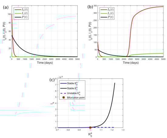
Figure 2. Dynamics of $I_h,I_v,P$ for (a) ${\beta }_{ch}=1.71859\times {10}^{-7}$ that corresponds to $(R_0^a<1)$, and (b) ${\beta }_{ch}=4.71859\times {10}^{-6}$ that corresponds to $(R_0^a>1)$. (a,b) Reducing cercaria infection rate on humans by limiting the number of contacts between susceptible humans and contaminated areas or by using self-protective gear when entering contaminated areas can decrease schistosomiasis prevalence. (c) Forward bifurcation diagram of System (2) in the case of the snail predator becoming extinct, showing that schistosomiasis is eradicated if $R_0^a<1$, but it becomes endemic if $R_0^a>1$.

5.2. Predator Survives

We next performed numerical simulations using $\tau =0.0001$ and ${\beta }_{ch}=1.914\times {10}^{-5}$, which implies that $\frac{\tau {\Pi }_v}{({\mu }_v+{\mu }_r){\mu }_p}=2.20543>1$. On the basis of the existence condition of the equilibrium points, the predator survives. In this case, the basic reproduction number is unity $(R_0^b=1)$ if the miracidia transmission rate on snails reaches its critical value, i.e., ${\beta }_{mv}^{*}=1.31409\times {10}^{-7}$. Hence, if we set ${\beta }_{mv}=0.31409\times {10}^{-7}<{\beta }_{mv}^{*}$, we obtain $k_1=2.43742>0$, $k_4=0.37218>0$, $k_6=0.01988>0$, $k_8=0.00045>0$, $k_9=3.1\times {10}^{-6}>0$, and $R_0^b=0.48889<1$. On the basis of Theorems 7 and 9, disease-free equilibrium point $\left(E_0^b\right)$ is asymptotically stable. This behavior was confirmed by our simulation, where the numerical solution was convergent to $\left(E_0^b\right)$; see Figure 3a. On the other hand, if we take ${\beta }_{mv}=4.31409\times {10}^{-7}>{\beta }_{mv}^{*}$, such that $R_0^b=1.81188>1$, then Theorem 8 shows that endemic equilibrium $\left(E_1^b\right)$ is asymptotically stable. The stability of $\left(E_1^b\right)$ is confirmed by Figure 3b, which shows that the numerical solution converges to $\left(E_1^b\right)$. When the predator goes extinct, schistosomiasis prevalence is higher than that when the predator survives. This means that the existence of a snail predator in the environment can reduce schistosomiasis prevalence.

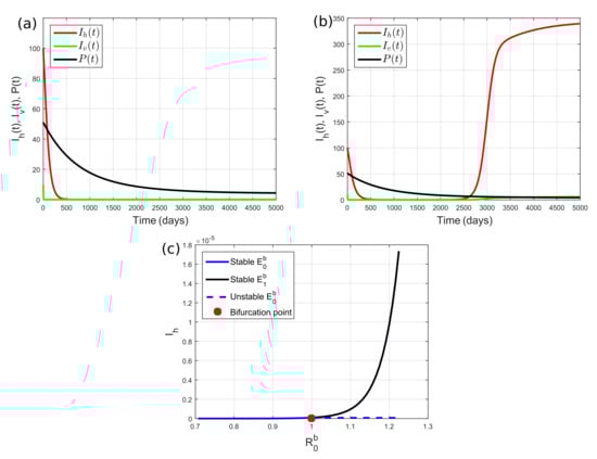
Figure 3. Dynamics of $I_h,I_v,P$ for (a) ${\beta }_{mv}=0.31409\times {10}^{-7}$, which corresponds to $R_0^b<1$; and (b) ${\beta }_{mv}=4.31409\times {10}^{-7}$, which corresponds to $R_0^b>1$. (a,b) Reducing miracidia transmission rate on snails by improving irrigation facilities (e.g., lining canals with cement) can reduce schistosomiasis prevalence. (c) Forward bifurcation diagram of System (2) in the case of snail predator surviving, showing that schistosomiasis is eradicated if $R_0^b<1$, but it becomes endemic if $R_0^b>1$.

Figure 3a,b indicate that there is an exchange of stability between the disease-free equilibrium point and the disease endemic equilibrium point when the miracidia transmission rate on snails is changed from ${\beta }_{mv}=0.31409\times {10}^{-7}<{\beta }_{mv}^{*}$ to ${\beta }_{mv}=4.31409\times {10}^{-7}>{\beta }_{mv}^{*}$. To more clearly see the effect of ${\beta }_{mv}$, we plotted in Figure 3c the steady state of $I_h$ against $R_0^b$. $R_0^b$ between $0.70710$ to $1.22474$ corresponding to ${\beta }_{mv}$ from $0.65704\times {10}^{-7}$ to $1.97114\times {10}^{-7}$; $R_0^b=1$ is obtained when ${\beta }_{mv}={\beta }_{mv}^{*}=1.31409\times {10}^{-7}$. Figure 3c shows that System (2) experiences forward bifurcation. Thus, $E_0^b$ is asymptotically stable, and $E_1^b$ does not exist when $R_0^b<1$. If $R_0^b>1$, $E_0^b$ becomes unstable, and $E_1^b$ exists and it is asymptotically stable.

5.3. Impact of Snail Predator as Biological Control Agent

We now investigate the impact of a snail predator as biological control agent. Here, we study the effect of predation rate $\left(\xi \right)$ by using parameter values as in Table 6: $\tau =0.0001$, ${\beta }_{ch}=0.1$ and ${\beta }_{mv}=4.31409\times {10}^{-7}$. According to [33], the predation rate is the proportion of prey killed per predator per time. It suggests that the predation rate is related to the effectiveness of the predator in hunting and killing snails. In this simulation, the basic reproduction number does not depend on the predation rate and is given by $R_0^b=18.11886$. Figure 4 shows that all numerical solutions using $\xi =0.1,\xi =0.15$, and $\xi =0.3$ are convergent to the same endemic equilibrium point. However, detailed observation shows that the schistosomiasis prevalence in the beginning of the intervention decreased as predation rate ($\xi$) increased. Several studies that are related to satiation-based predation models show that the predation rate is related to the gut capacity of the predator [34]. Hence, we should use snail predators that can effectively hunt and kill snails, and have high gut capacity.

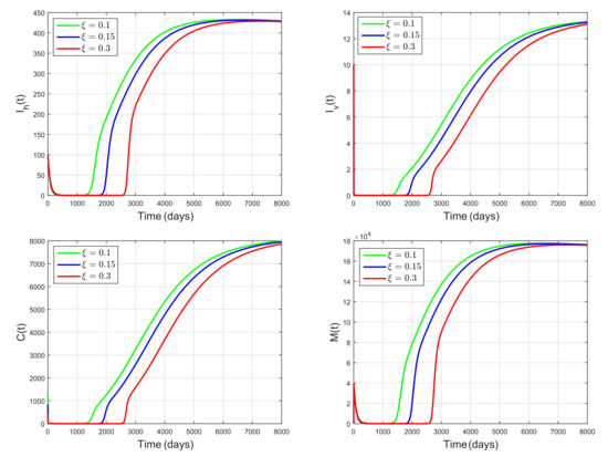
Figure 4. Dynamics of $I_h$, $I_v$, C, M for $\xi =0.1,0.15,0.3$, showing that the effectiveness of predators in hunting and killing snails plays an important role in reducing schistosomiasis prevalence at the beginning of intervention.

We next investigate the influence of conversion rate $\tau$ by performing simulations using the same parameter values as those in Figure 4, but with varying $\tau$ and fixed $\xi =0.01$. According to [35], the conversion rate is related to the efficiency in turning predation into new predators. It implies that the conversion rate is related to the birth rate of snail predator. By choosing $\tau =0.0001$, $\tau =0.00015$, and $\tau =0.0003$, we get the basic reproduction number $\left(R_0^b\right)=18.118869$, $\left(R_0^b\right)=12.07924$, $\left(R_0^b\right)=6.03962$, respectively. Hence, the basic reproduction number decreases as $\tau$ increases. The dynamics of $I_h$, $I_v$, C, and M for $\tau =0.0001,0.00015$, and $0.0003$ is shown in Figure 5. Values of the steady state of $I_h$, $I_v$, C, and M were smaller for larger values of $\tau$. Thus, schistosomiasis prevalence decreases as $\tau$ increases. So, the snail-predator birth rate plays an essential role in controlling schistosomiasis spread. Figure 4 and Figure 5 show that using a natural predator of snails as a biological control agent can decrease schistosomiasis prevalence. These results are in line with the results in [7].

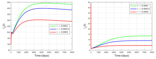
Figure 5. Dynamics of $I_h$, $I_v$, C, M for $\tau =0.0001,0.00015,0.0003$, showing that the conversion rate of the snail predator that is related to its birth rate plays an essential role in reducing schistosomiasis prevalence.

6. Conclusions

In this work, a deterministic schistosomiasis model incorporating a snail predator as a biological control agent was discussed. The existence and stability conditions of all equilibrium points were investigated. Our findings suggest that a snail predator as a biological control agent can reduce the prevalence of schistosomiasis. Moreover, our results showed that the snail-predator birth rate plays an important role in controlling schistosomiasis spread. Despite the contributions of our work, it has some limitations. Due to the lack of data related to the parameters of our model, we only chose parameter values by considering the results of qualitative analysis, i.e., the existence and stability conditions of the equilibrium points. For further research, sensitivity and cost-effectiveness analysis of the interventions discussed in our proposed model will be considered.

References

- Ross, A.G.; Chau, T.N.; Inobaya, M.T.; Olveda, R.M.; Li, Y.; Harn, D.A. A new global strategy for the elimination of schistosomiasis. Int. J. Infect. Dis. 2017, 54, 130–137. [Google Scholar] [CrossRef]
- WHO. Schistosomiasis: Progress Report 2001–2011, Strategic Plan 2012–2020; World Health Organization Press: Geneva, Switzerland, 2013; p. 74. [Google Scholar]
- Rollinson, D.; Knopp, S.; Levitz, S.; Stothard, J.R.; Tchuem Tchuenté, L.A.; Garba, A.; Mohammed, K.A.; Schur, N.; Person, B.; Colley, D.G.; et al. Time to set the agenda for schistosomiasis elimination. Acta Trop. 2013, 128, 423–440. [Google Scholar] [CrossRef]
- Arostegui, M.C.; Wood, C.L.; Jones, I.J.; Chamberlin, A.J.; Jouanard, N.; Faye, D.S.; Kuris, A.M.; Riveau, G.; De Leo, G.A.; Sokolow, S.H. Potential Biological Control of Schistosomiasis by Fishes in the Lower Senegal River Basin. Am. J. Trop. Med. Hyg. 2019, 100, 117–126. [Google Scholar] [CrossRef]
- Coelho, P.; Caldeira, R. Critical analysis of molluscicide application in schistosomiasis control programs in Brazil. Infect. Dis. Poverty 2016, 5, 57. [Google Scholar] [CrossRef]
- King, C.H.; Bertsch, D. Historical Perspective: Snail Control to Prevent Schistosomiasis. PLoS Negl. Trop. Dis. 2015, 9, e0003657. [Google Scholar] [CrossRef]
- Sokolow, S.H.; Huttinger, E.; Jouanard, N.; Hsieh, M.H.; Lafferty, K.D.; Kuris, A.M.; Riveau, G.; Senghor, S.; Thiam, C.; N’Diaye, A.; et al. Reduced transmission of human schistosomiasis after restoration of a native river prawn that preys on the snail intermediate host. Proc. Natl. Acad. Sci. USA 2015, 112, 9650–9655. [Google Scholar] [CrossRef]
- Sokolow, S.H.; Wood, C.L.; Jones, I.J.; Swartz, S.J.; Lopez, M.; Hsieh, M.H.; Lafferty, K.D.; Kuris, A.M.; Rickards, C.; De Leo, G.A. Global assessment of schistosomiasis control over the past century shows targeting the snail intermediate host works best. PLoS Negl. Trop. Dis. 2016, 10, e0004794. [Google Scholar] [CrossRef] [PubMed]
- MacDonald, G. The dynamics of helminth infections, with special reference to schistosomes. Trans. R. Soc. Trop. Med. Hyg. 1965, 59, 489–506. [Google Scholar] [CrossRef]
- Chiyaka, E.T.; Garira, W. Mathematical Analysis of the Transmission Dynamics of Schistosomiasis in the Human-Snail Hosts. J. Biol. Syst. 2009, 17, 397–423. [Google Scholar] [CrossRef]
- Gao, S.; Liu, Y.; Luo, Y.; Xie, D. Control problems of a mathematical model for schistosomiasis transmission dynamics. Nonlinear Dyn. 2011, 63, 503–512. [Google Scholar] [CrossRef]
- Ding, C.; Sun, Y.; Zhu, Y. A schistosomiasis compartment model with incubation and its optimal control. Math. Methods Appl. Sci. 2017, 40, 5079–5094. [Google Scholar] [CrossRef]
- Nur, W.; Trisilowati; Suryanto, A.; Kusumawinahyu, W.M. Mathematical model of schistosomiasis with health education and molluscicide intervention. J. Phys. Conf. Ser. 2021, 1821, 012033. [Google Scholar] [CrossRef]
- Nur, W.; Trisilowati; Suryanto, A.; Kusumawinahyu, W.M. Mathematical Modelling of Schistosomiasis Transmission Dynamics in Traditional Cattle Farmer Communities. In Proceedings of the 1st International Conference on Mathematics and Mathematics Education (ICMMEd 2020), Ambon, Indonesia, 26 November 2020; Atlantis Press: Dordrecht, The Netherlands, 2021; pp. 462–470. [Google Scholar] [CrossRef]
- Diaby, M.; Iggidr, A.; Sy, M.; Sène, A. Global analysis of a schistosomiasis infection model with biological control. Appl. Math. Comput. 2014, 246, 731–742. [Google Scholar] [CrossRef][Green Version]
- Okamoto, K.W.; Amarasekare, P. The biological control of disease vectors. J. Theor. Biol. 2012, 309, 47–57. [Google Scholar] [CrossRef]
- Okamoto, K.W.; Gould, F.; Lloyd, A.L. Integrating Transgenic Vector Manipulation with Clinical Interventions to Manage Vector-Borne Diseases. PLoS Comput. Biol. 2016, 12, e1004695. [Google Scholar] [CrossRef][Green Version]
- Lemos-Paião, A.P.; Silva, C.J.; Torres, D.F. A cholera mathematical model with vaccination and the biggest outbreak of world’s history. AIMS Math. 2018, 3, 448–463. [Google Scholar] [CrossRef]
- Castillo-Chavez, C.; Song, B. Dynamical Models of Tuberculosis and Their Applications. Math. Biosci. Eng. 2004, 1, 361–404. [Google Scholar] [CrossRef]
- Nelwan, M.L. Schistosomiasis: Life Cycle, Diagnosis, and Control. Curr. Ther. Res. 2019, 91, 5–9. [Google Scholar] [CrossRef]
- Gryseels, B.; Polman, K.; Clerinx, J.; Kestens, L. Human schistosomiasis. Lancet 2006, 368, 1106–1118. [Google Scholar] [CrossRef]
- Bergquist, R.; Zhou, X.N.; Rollinson, D.; Reinhard-Rupp, J.; Klohe, K. Elimination of schistosomiasis: The tools required. Infect. Dis. Poverty 2017, 6, 158. [Google Scholar] [CrossRef] [PubMed]
- Li, H.; Guo, S. Dynamics of A SIRC Epidemiological Model. Electron. J. Erential Equ. 2017, 2017, 1–18. [Google Scholar]
- Yang, X.; Chen, L.; Chen, J. Permanence and positive periodic solution for the single-species nonautonomous delay diffusive models. Comput. Math. Appl. 1996, 32, 109–116. [Google Scholar] [CrossRef]
- van den Driessche, P.; Watmough, J. Reproduction numbers and sub-threshold endemic equilibria for compartmental models of disease transmission. Math. Biosci. 2002, 180, 29–48. [Google Scholar] [CrossRef]
- Polyanin, A.D.; Manzhirov, A.V. Handbook of Mathematics for Engineers and Scientists; Chapman and Hall/CRC: Boca Raton, FL, USA, 2007. [Google Scholar]
- Cook, M.Y. Flight Dynamics Principles, 2nd ed.; Elsevier: Oxford, UK, 2007. [Google Scholar]
- Marghitu, D. Mechanical Enginer’s Handbook; Academic Press: San Diego, CA, USA, 2001. [Google Scholar]
- Liénard, A.; Chipart, M.H. Sur le signe de la partie réelle des racines d’une équation algébrique. J. Math. Pures Appl. 1914, 10, 291–346. [Google Scholar]
- Meiss, J.D. Differential Dynamical Systems; Society for Industrial and Applied Mathematics: New York, NY, USA, 2007. [Google Scholar] [CrossRef]
- Lundström, N.L.P. How to find simple nonlocal stability and resilience measures. Nonlinear Dyn. 2018, 93, 887–908. [Google Scholar] [CrossRef]
- van Kan, A.; Jegminat, J.; Donges, J.F.; Kurths, J. Constrained basin stability for studying transient phenomena in dynamical systems. Phys. Rev. E 2016, 93, 042205. [Google Scholar] [CrossRef]
- Vucetich, J.A.; Hebblewhite, M.; Smith, D.W.; Peterson, R.O. Predicting prey population dynamics from kill rate, predation rate and predator-prey ratios in three wolf-ungulate systems. J. Anim. Ecol. 2011, 80, 1236–1245. [Google Scholar] [CrossRef] [PubMed]
- Metz, J.A.J.; Sabelis, M.W.; Kuchlein, J.H. Sources of variation in predation rates at high prey densities: An analytic model and a mite example. Exp. Appl. Acarol. 1988, 5, 187–205. [Google Scholar] [CrossRef]
- Han, L.; Ma, Z.; Hethcote, H. Four predator prey models with infectious diseases. Math. Comput. Model. 2001, 34, 849–858. [Google Scholar] [CrossRef]
Publisher’s Note: MDPI stays neutral with regard to jurisdictional claims in published maps and institutional affiliations. |
© 2021 by the authors. Licensee MDPI, Basel, Switzerland. This article is an open access article distributed under the terms and conditions of the Creative Commons Attribution (CC BY) license (https://creativecommons.org/licenses/by/4.0/).