Optimal Price and Lot Size for an EOQ Model with Full Backordering under Power Price and Time Dependent Demand

Abstract

In this paper, we address an inventory system where the demand rate multiplicatively combines the effects of time and selling price. It is assumed that the demand rate is the product of two power functions, one depending on the selling price and the other on the time elapsed since the last inventory replenishment. Shortages are allowed and fully backlogged. The aim is to obtain the lot sizing, the inventory cycle and the unit selling price that maximize the profit per unit time. To achieve this, two efficient algorithms are proposed to obtain the optimal solution to the inventory problem for all possible parameter values of the system. We solve several numerical examples to illustrate the theoretical results and the solution methodology. We also develop a numerical sensitivity analysis of the optimal inventory policy and the maximum profit with respect to the parameters of the demand function.

1. Introduction

Inventory Theory collects a set of mathematical models which describe the properties of a wide variety of inventory systems, and studies different methodologies to seek and analyze the best strategies that may be applied in the management of inventories. In the literature on inventory models, the demand rate of items is often assumed to be constant and known, independent of the time elapsed since the last replenishment. Thus, Chung et al. [1] provide the optimal solution for an inventory model with lot-size-dependent trade credit under delayed payment, cash discount and constant demand rate. Vandana and Sharma [2] developed an inventory model with constant demand, partial backlogging and partial permissible delay-in-payment. Mokhtari [3] proposed an economic order quantity model with constant demand to determine the joint ordering policy for two products under completion and substitution. Other recent papers considering constant demand are the following: Lin et al. [4], Chung et al. [5], Khakzad and Gholamian [6] and Mishra et al. [7].

However, for some types of products, the demand rate often depends on time or/and other characteristics. For this reason, in this paper, we develop an inventory model to determine the optimal policy for products in which demand depends on time and the selling price of the item. Thus, the demand rate is the product of a power time-function and a decreasing price-function. This price-function is a power-function that depends on several parameters and represents the relation between demand and the unit selling price. The power time-dependent demand pattern was introduced by Naddor [8] and, since then, several papers have appeared in the literature with this type of demand. Among others, we can cite the papers of Datta and Pal [9], Lee and Wu [10], Rajeswari and Vanjikkodi [11], Mishra et al. [12], Singh and Kumar [13], Mishra and Singh [14] and Rajeswari and Indrani [15]. A common characteristic of all the above papers is that the length of the inventory cycle is fixed. Later on, Sicilia et al. [16,17], San-José et al. [18], Adaraniwon and Omar [19,20] and San-José et al. [21] developed inventory systems with a power demand pattern in which the inventory cycle is not fixed and is, therefore, a decision variable of the inventory problem. Demand rate as a separable function of time and the selling price was also introduced in some articles on inventory management. Thus, the papers developed by Smith et al. [22], Soni [23], Wu et al. [24], Avinadav et al. [25], San-José et al. [26] and Pando et al. [27] considered this assumption.

In some real inventory systems, it may be more advantageous for the firm that the customers have to wait a time period until the arrival of the next replenishment to receive their orders. Thus, in this paper, we assume that shortages are allowed and completely backordered. That is, any customer arriving in the stock-out period is willing to wait for the next replenishment. This hypothesis of full backordering is also considered in other papers (see, e.g., San-José and García-Laguna [28], Birbil et al. [29], Jakic and Fransoo [30], Mishra et al. [31] and San-José et al. [32]).

In the inventory literature, we know of no papers on inventory systems that simultaneously assume the following characteristics: demand rate is the product of a time-dependent power demand and a price-dependent power demand, shortages are completely backordered and the length of the inventory cycle is a decision variable. The inventory system studied here is based on these assumptions. The objective function to optimize is the profit per unit time. This profit is calculated by the difference between the revenue from product sales and the sum of ordering cost, purchasing cost, holding cost and backordering cost. The aim is to determine the optimal inventory policy (the economic lot size and optimal inventory cycle) and the optimal selling price that maximize the total profit per unit time. Under the above considerations, a new approach is developed for determining the optimal policy and the best selling-price of the product, taking into account the values of the parameters considered in the inventory system.

The outline of the paper is described below. Section 2 specifies the hypothesis of the model and the notation used in the rest of the work. Section 3 presents the mathematical formulation, including the calculation of costs related to the management of the inventory system and the establishment of the profit function per unit of time. Section 4 studies some properties of the objective function and develops algorithmic procedures that allow to determine the optimal inventory policy for the two different situations that can occur. In Section 5, we introduce some numerical examples to illustrate the application of the optimization procedures. Moreover, we also give a numerical sensitivity analysis for the best selling price, the optimal inventory policy and maximum profit with respect to the parameters of the demand rate function. Finally, in Section 6, we provide the conclusions of this paper and possible future research directions in this area.

2. Hypothesis and Notation

The inventory system analyzed in this work has the following properties:

• The inventory system considers a single item.
• Inventory control is performed through a continuous review system.
• The replenishment period is negligible or null.
• The planning horizon is infinite.
• The lead-time is zero.
• The inventory is scheduled each T time unit. It is a decision variable.
• The cost of placing an order is constant and independent of the size of the order.
• The unit purchasing cost is known and constant.
• The unit selling price is unknown and it is a decision variable.
• The unit holding cost is a linear function of the time that the article remains in the store.
• Shortages are allowed and completely backlogged.
• The unit cost of shortage is a linear function of the time that elapses until the item is received.
• The inventory is replenished when the number of backorders is equal to $-s$ quantity units. That is, the reorder level is s.
• The replenishment size Q raises the inventory at the beginning of each scheduling period to the order level S.
• Demand $D(t,p)$ is a function that depends on time and the selling price of the item. It is assumed that

  $$D(t,p)=D_1\left(t\right)D_2\left(p\right),$$

  that is, demand combines the effects of time and the selling price in a multiplicative way.

In this paper, it is assumed that $D_1\left(t\right)$ is a power function given by

$$D_1(t)=\frac{1}{n}{\left(\frac{t}{T}\right)}^{1/n-1},0<t<T$$

(1)

with index $n>0$, and $D_2\left(p\right)$ is a decreasing power function given by

$$D_2\left(p\right)=\alpha -\beta p^{\gamma },\mathrm{with}\alpha >0,\beta >0\mathrm{and}\gamma >0.$$

(2)

The parameter $\alpha$ represents the market size and the parameters $\beta$ and $\gamma$ are the coefficients related to the sensibility of demand with respect to the unit selling price. As $D(t,p)\ge 0$, then the maximum unit selling price is

$$p_m={\left(\frac{\alpha }{\beta }\right)}^{1/\gamma }$$

(3)

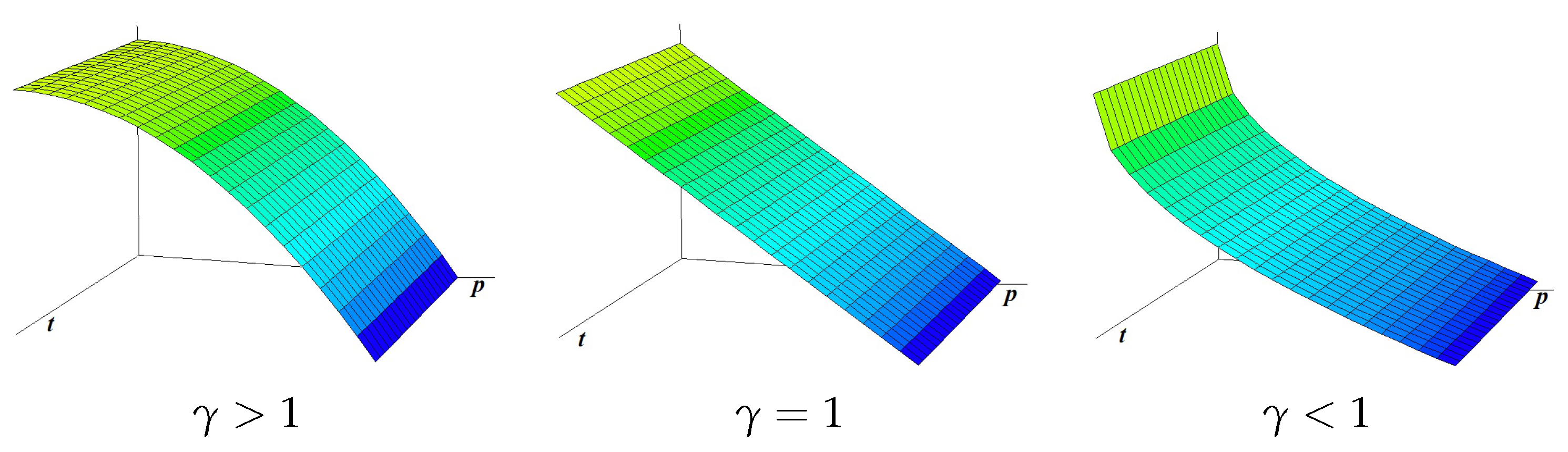
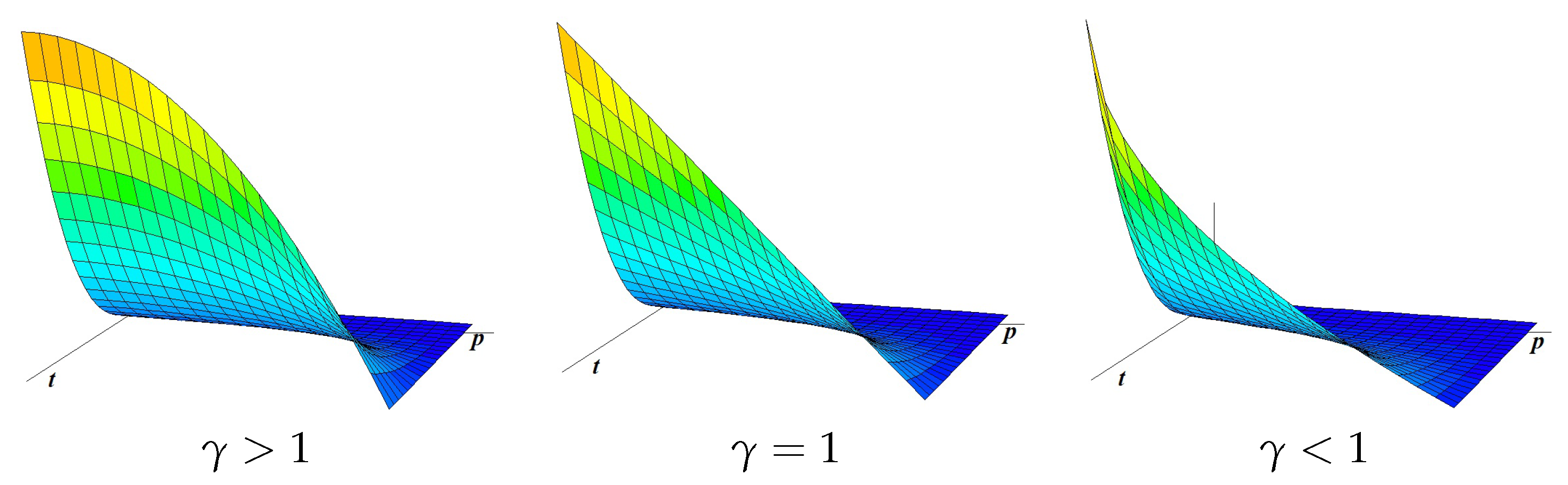
Note that the demand patterns represent the different ways by which quantities are taken out of inventory to fill customer demand. Given p, the function $D(t,p)$ is known as the power demand pattern. Depending on the value of the index n, that function $D(t,p)$ may represent several ways in which demand occurs during an inventory cycle (see, e.g., Naddor [8], Mishra et al. [12], Singh and Kumar [13], Rajeswari and Indrani [15], Sicilia et al. [16,17], and San-José et al. [18,21,32]). Thus, if $\mathit{n}>1$, then this means that demand is large at the beginning of the scheduling period and then declines throughout the inventory cycle. If $\mathit{n}=1$, the demand is constant throughout the scheduling period. Finally, if $\mathit{n}<1$, then demand is very low at the beginning of the scheduling period and then increases throughout the inventory cycle, reaching the highest demand at the end of the cycle.

Figure 1, Figure 2 and Figure 3 plot the demand rate function $D(t,p)$ for different values of the parameters $\gamma$ and n.

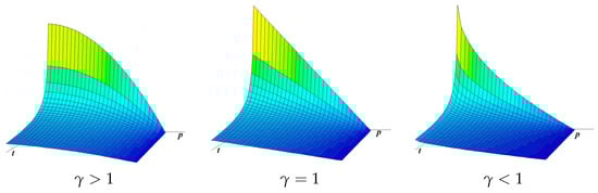
Figure 1. Demand functions $D(t,p)$ when $n>1$.

Figure 2. Demand functions $D(t,p)$ when $n=1$.

Figure 3. Demand functions $D(t,p)$ when $n<1$.

The notation used throughout this work is shown in Table 1.

Table 1. Notation.

$\varphi$	Stock-in period (≥0)
$\sigma$	Stock-out period (≥0)
T	Length of inventory cycle, that is, $T=\varphi +\sigma$ (>0, decision variable)
Q	Lot size or replenishment size (>0)
S	Maximum inventory level (≥0, decision variable)
s	Reorder point (≤0)
c	Unit purchasing cost (>0)
p	Unit selling price $(p\ge c,$ decision variable)
A	The cost of placing an order (>0)
h	The unit holding cost per time unit (>0)
$\pi$	The unit backordering cost per time unit (>0)
$D(t,p)$	Demand at time t when the unit selling price is p, for $0<t<T$
$I(t,p)$	Inventory level at time t when the unit selling price is p, for $0\le t<T$
n	Index of the power demand pattern (>0)
$G(S,T,p)$	Total Profit per unit time
$B\left(p\right)$	The optimum profit per unit time for a fixed p, that is, $B\left(p\right)=$ $G(S^{*}\left(p\right),T^{*}\left(p\right),p)$

In the next section, we determine the inventory level function $I(t,p)$, which describes the evolution of the net inventory, and the costs related to the inventory system.

3. Formulation of the Mathematical Model

The fluctuation of the inventory level during the inventory cycle T is as follows: At the beginning of the scheduling period, there are S units in stock. That amount decreases due to demand during the interval $(0,\varphi ]$ and drops to zero at $t=\varphi$. Thus, we have

$$S={\int }_0^{\varphi }D(t,p)dt.$$

(4)

Next, during the interval $[\varphi ,T]$, the inventory level decreases continuously due to the effect of customer demand. During this period there is no stock, shortages occur and demand is backlogged. When the on-hand inventory level is equal to s (reorder point), a new replenishment is added to the inventory and a new inventory cycle begins. Hence, the inventory level at any instant of time t during $[0,T]$ is described by

$$I(t,p)=S-{\int }_0^{t}D(t,p)dt=D_2\left(p\right){\int }_t^{\varphi }{D}_1\left(t\right)dt.$$

(5)

From (1) and (2), substituting the functions $D_1\left(t\right)$ and $D_2\left(p\right)$ into (5), we have

$$I(t,p)=\left(\alpha -\beta p^{\gamma }\right)T\left[{\left(\frac{\varphi }{T}\right)}^{1/n}-{\left(\frac{t}{T}\right)}^{1/n}\right]=S-\left(\alpha -\beta p^{\gamma }\right)T{\left(\frac{t}{T}\right)}^{1/n}.$$

(6)

As at point $t=0$ the inventory level is equal to S, then we have

$$S=\left(\alpha -\beta p^{\gamma }\right)T{\left(\frac{\varphi }{T}\right)}^{1/n}$$

(7)

Also, at the point $t=T$, the inventory level coincides to the reorder point, that is, $s=I(T,p)$. Hence, we obtain

$$s=I(T,p)=\left(\alpha -\beta p^{\gamma }\right)T\left[{\left(\frac{\varphi }{T}\right)}^{1/n}-1\right].$$

(8)

The lot size Q is equal to $S-s$. Thus, from (7) and (8), we have

$$Q=\left(\alpha -\beta p^{\gamma }\right)T.$$

(9)

The Objective Function

Let $G(S,T,p)$ be the profit per unit time. That profit is equal to the revenues per cycle ($pQ$) minus the sum of the costs related to the inventory management. These costs are the purchasing cost ($cQ$), the ordering cost (A), the holding cost ($HC$) and the shortage cost ($SC$). The holding cost is given by

$$HC=h{\int }_0^{\varphi }I(t,p)dt=\frac{h}{n+1}ST{\left(\frac{S}{\left(\alpha -\beta p^{\gamma }\right)T}\right)}^n$$

(10)

and the shortage cost is

$$SC=\pi {\int }_{\varphi }^T\left[-I(t,p)\right]dt=\pi \left[\frac{n}{n+1}\left(\alpha -\beta p^{\gamma }\right)T^2-ST+\frac{1}{n+1}ST{\left(\frac{S}{\left(\alpha -\beta p^{\gamma }\right)T}\right)}^n\right].$$

(11)

Hence, the profit per time unit is given by

$$\begin{array}{ccc}G(S,T,p)\hfill & =\hfill & \frac{1}{T}\left[(p-c)Q-A-h{\int }_0^{\varphi }I(t,p)dt+\pi {\int }_{\varphi }^{T}I(t,p)dt\right]\hfill \\ \hfill & =\hfill & (p-c)\left(\alpha -\beta p^{\gamma }\right)-\frac{A}{T}-\frac{h+\pi }{n+1}S{\left(\frac{S}{\left(\alpha -\beta p^{\gamma }\right)T}\right)}^n\hfill \\ \hfill & \hfill & -\frac{n}{n+1}\pi \left(\alpha -\beta p^{\gamma }\right)T+\pi S\hfill \end{array}$$

(12)

Our goal is to determine the values of the decision variables S, T and p that maximize the profit $G(S,T,p)$ per unit time, subject to the constraints $T>0$, $0\le S\le \left(\alpha -\beta p^{\gamma }\right)T$ and $c\le p\le p_m$, with $p_m$ given by (3).

4. Analysis of the Inventory Problem

It is easy to check that, for a fixed p, the function $G(S,T,p)$ is strictly concave and has a maximum point $(S^{*}\left(p\right),T^{*}\left(p\right))$ determined by

$$\begin{array}{ccc}\hfill S^{*}\left(p\right)& =& {\left(\frac{\pi }{h+\pi }\right)}^{1/n}\left(\alpha -\beta p^{\gamma }\right)\sqrt{\frac{(n+1)A}{n\left(\alpha -\beta p^{\gamma }\right)\pi \left(1-{\left(\frac{\pi }{h+\pi }\right)}^{1/n}\right)}}\hfill \end{array}$$

(13)

$$\begin{array}{ccc}\hfill T^{*}\left(p\right)& =& \sqrt{\frac{(n+1)A}{n\left(\alpha -\beta p^{\gamma }\right)\pi \left(1-{\left(\frac{\pi }{h+\pi }\right)}^{1/n}\right)}}\hfill \end{array}$$

(14)

Thus, given p, the optimum profit per unit time is

$$B\left(p\right)=G(S^{*}\left(p\right),T^{*}\left(p\right),p)=(p-c)\left(\alpha -\beta p^{\gamma }\right)-2\sqrt{\alpha -\beta p^{\gamma }}\theta ,$$

(15)

where the auxiliary parameter $\theta$ is given by

$$\theta =\sqrt{\frac{n}{n+1}A\pi \left(1-{\left(\frac{\pi }{h+\pi }\right)}^{1/n}\right)}.$$

(16)

The function $B\left(p\right)$ has the following properties:

(i)

$B\left(p\right)$ is continuous on the interval $[c,p_m]$. Moreover, $B\left(c\right)<0$ and $B\left(p_m\right)=0$.

(ii)

$B\left(p\right)$ is differentiable and its derivative is

$$\begin{array}{ccc}{B}^{\prime }\left(p\right)\hfill & =\hfill & \alpha +\beta p^{\gamma -1}\left(\gamma c+\frac{\gamma \theta }{\sqrt{\alpha -\beta p^{\gamma }}}-(\gamma +1)p\right)\hfill \\ \hfill & =\hfill & \beta p^{\gamma -1}\left(\frac{\alpha }{\beta }{p}^{1-\gamma }+\gamma c+\frac{\gamma \theta }{\sqrt{\alpha -\beta p^{\gamma }}}-(\gamma +1)p\right)\hfill \end{array}$$

(17)

(iii)

Sign$\left(B^{\prime }\left(p\right)\right)=$ sign$\left(f\right(p\left)\right)$, where the function $f\left(p\right)$ is defined by

$$f\left(p\right)=\gamma c-(\gamma +1)p+\frac{\alpha }{\beta }{p}^{1-\gamma }+\frac{\gamma \theta }{\sqrt{\alpha -\beta p^{\gamma }}}.$$

(18)

Thus, the maximum of the function $B\left(p\right)$ can be found by analyzing the function $f\left(p\right)$. For that, we calculate the two first derivatives of the function $f\left(p\right)$:

$$f^{\prime }\left(p\right)=-(\gamma +1)+\frac{\alpha }{\beta }\left(1-\gamma \right)p^{-\gamma }+\frac{\beta {\gamma }^2\theta p^{\gamma -1}}{2\sqrt{{\left(\alpha -\beta p^{\gamma }\right)}^3}}$$

(19)

and

$$f^{″}\left(p\right)=\left(\gamma -1\right)\left(\frac{\alpha \gamma }{\beta }{p}^{-\left(\gamma +1\right)}+\frac{\alpha \beta {\gamma }^2\theta p^{\gamma -2}}{2\sqrt{{\left(\alpha -\beta p^{\gamma }\right)}^5}}\right)+\frac{\left(\gamma +2\right){\beta }^2{\gamma }^2\theta p^{2\left(\gamma -1\right)}}{4\sqrt{{\left(\alpha -\beta p^{\gamma }\right)}^5}}.$$

(20)

Next, we study separately two scenarios: when $\gamma \ge 1$ and when $0<\gamma <1$.

4.1. Optimum Solution for the Case $\gamma \ge 1$

In this scenario the function $f\left(p\right)$ is strictly convex. Thus, the optimum value of the unit selling price p is determined by the following result.

Theorem 1.

Let $B\left(p\right)$, $f\left(p\right)$ and $f^{\prime }\left(p\right)$ be the functions given by (15), (18) and (19), respectively. When $\gamma \ge 1$, the optimal inventory policy is as follows:

1. 

If $f^{\prime }\left(c\right)$ is non-negative, then the optimum unit selling price is $p^{*}=p_m$ and the maximum profit per unit time is $B^{*}=B\left(p^{*}\right)=0$.

2. 

Otherwise $\left(f^{\prime }\left(c\right)<0\right)$, let $p_1={arg}_{p\in (c,p_m)}\{f^{\prime }\left(p\right)=0\}$.

(a) 

If $f\left(p_1\right)\ge 0$, then $p^{*}=p_m$ and $B^{*}=B\left(p_m\right)=0$.

(b) 

If $f\left(p_1\right)<0$, then to let $p_0={arg}_{p\in (c,p_1)}\{f\left(p\right)=0\}$.

i. 

If $B\left(p_0\right)<0$, then $p^{*}=p_m$ and $B^{*}=B\left(p^{*}\right)=0$.

ii. 

If $B\left(p_0\right)\ge 0$, then $p^{*}=p_0$ and the maximum profit per unit time is $B^{*}=B\left(p_0\right)=(p_0-c)\left(\alpha -\beta p_0^{\gamma }\right)-2\theta \sqrt{\alpha -\beta p_0^{\gamma }}$.

Proof. 

Please see the proof in the Appendix A. □

Remark 1.

From Theorem 1, the optimal selling price $p^{*}$ when $\gamma \ge 1$ is either $p_m$ or $p_0={arg}_{p\in (c,p_1)}\{f\left(p\right)=0\}$. This optimum price $p^{*}$ depends whether the values $f^{\prime }\left(c\right)$, $f\left(p_1\right)$ and $B\left(p_0\right)$ are positive or not.

Taking into account Theorem 1, the following algorithmic procedure gives the optimal inventory policy when $\gamma \ge 1$.

4.2. Optimum Solution for the Case $0<\gamma <1$

Consider now the scenario where $0<\gamma <1$. In this case, the curvature of the function $f\left(p\right)$ is unknown. For that, we have to study the behavior of the derivative of the function $f\left(p\right)$.

Lemma 1.

The function $f^{\prime }\left(p\right)$ given by (19) is strictly convex.

Proof. 

Please see the Appendix A. □

Note that if $0<\gamma <1$, then the function $f^{\prime }\left(p\right)$ has at most two zeros. Therefore, the function $f\left(p\right)$ has at most two local extreme points in the interval $(c,p_m)$. Taking into account this property, the optimal inventory policy when $0<\gamma <1$ is presented in the following result.

Theorem 2.

Let $B\left(p\right)$, $f\left(p\right)$, $f^{\prime }\left(p\right)$ and $f^{″}\left(p\right)$ be the functions given by (15), (18)–(20), respectively. Suppose that $0<\gamma <1$. The optimal inventory policy is as follows:

1. 

If $f^{\prime }\left(c\right)\ge 0$ and $f^{″}\left(c\right)\ge 0$, then the optimum unit selling price is $p^{*}=p_m$ and the maximum profit is $B^{*}=B\left(p_m\right)=0$.

2. 

If $f^{\prime }\left(c\right)\ge 0$ and $f^{″}\left(c\right)<0$, then to let $p_2={arg}_{p\in (c,p_m)}\{f^{″}\left(p\right)=0\}$.

(a) 

If $f^{\prime }\left(p_2\right)\ge 0$, then $p^{*}=p_m$ and $B^{*}=B\left(p_m\right)=0$.

(b) 

If $f^{\prime }\left(p_2\right)<0$, then to let $p_3={arg}_{p\in (c,p_2)}\{f^{\prime }\left(p\right)=0\}$ and

$p_4={arg}_{p\in (p_2,p_m)}\{f^{\prime }\left(p\right)=0\}$.

i. 

If $f\left(p_4\right)\ge 0$, then $p^{*}=p_m$ and $B^{*}=B\left(p_m\right)=0$.

ii. 

If $f\left(p_4\right)<0$, then to let $p_5={arg}_{p\in (p_3,p_4)}\{f\left(p\right)=0\}$.

(A)

If $B\left(p_5\right)<0$, then $p^{*}=p_m$ and $B^{*}=B\left(p_m\right)=0$.

(B)

If $B\left(p_5\right)\ge 0$, then $p^{*}=p_5$ and the maximum profit is given by $B^{*}=B\left(p_5\right)=p_5-c)\left(\alpha -\beta p_5^{\gamma }\right)-2\theta \sqrt{\alpha -\beta p_5^{\gamma }}$.

3. 

If $f^{\prime }\left(c\right)<0$, then to let $p_1={arg}_{p\in (c,p_m)}\{f^{\prime }\left(p\right)=0\}$.

(a) 

If $f\left(p_1\right)\ge 0$, then $p^{*}=p_m$ and $B^{*}=B\left(p_m\right)=0$.

(b) 

If $f\left(p_1\right)<0$, let $p_0={arg}_{p\in (c,p_1)}\{f\left(p\right)=0\}$.

i. 

If $B\left(p_0\right)<0$, then $p^{*}=p_m$ and $B^{*}=B\left(p_m\right)=0$.

ii. 

If $B\left(p_0\right)\ge 0$, then $p^{*}=p_0$ and the maximum profit is $B^{*}=B\left(p_0\right)=(p_0-c)\left(\alpha -\beta p_0^{\gamma }\right)-2\theta \sqrt{\alpha -\beta p_0^{\gamma }}$.

Proof. 

Please see Appendix A. □

Remark 2.

From Theorem 2, the optimal selling price $p^{*}$ when $0<\gamma <1$ is $p_m$, $p_0={arg}_{p\in (c,p_1)}\{f\left(p\right)=0\}$, or $p_5={arg}_{p\in (p_3,p_4)}\{f\left(p\right)=0\}$. This optimum price $p^{*}$ is conditioned by the sign of the values $f^{\prime }\left(c\right)$, $f^{″}\left(c\right)$, $f\left(p_1\right)$, $f\left(p_4\right)$, $f^{\prime }\left(p_2\right)$, $B\left(p_0\right)$ and $B\left(p_5\right)$.

The following algorithmic approach determines the optimum inventory policy when $0<\gamma <1$.

Remark 3.

Note that if $p^{*}=p_m$, then the inventory system is unprofitable.

4.3. Particular Models

In this subsection, we comment that some models studied by other authors are specific cases from the model proposed in this paper.

(1)

If we consider $\beta \to 0$, then we have the inventory model with power demand pattern and full backlogging analyzed by Sicilia et al. [16].

(2)

If we assume that $n=1$ and $\beta \to 0$, then the inventory problem is reduced to ${max}_{\begin{array}{c}0\le b\le Q\\ Q>0\end{array}}{G}_0(Q,b)=(p-c)\alpha -A\frac{\alpha }{Q}-h\frac{{(Q-b)}^2}{2Q}-\pi \frac{b^2}{2Q}$, where $b=-s$, that is, we derive to the EOQ model with full backordeing (see, e.g., Axsäter [33], p. 31).

(3)

Considering that $n=1$, $\gamma =1$ and $\pi \to \infty$, we derive using the models developed by Smith et al. [22], and Kunreuther and Richard [34] when a linear demand is assumed. Besides, the optimal policy determined by Algorithm 1 is equal to the “simultaneous solution” proposed by the cited authors.

(4)

Also, when $n=1$, $\gamma =1$ and $\pi \to \infty$, we obtain the model studied by Kabirian [35] if we suppose that the demand rate is constant, the production cost is fixed and the production rate is infinite.

Algorithm 1  Obtaining the optimal policy and the maximum profit when $\gamma \ge 1$
Step 1	From (19), calculate $f^{\prime }\left(c\right)$.
Step 2	If $f^{\prime }\left(c\right)\ge 0$, then go to step 8. Otherwise, go to step 3.
Step 3	Obtain $p_1={arg}_{p\in (c,p_m)}\{f^{\prime }\left(p\right)=0\}$.
Step 4	If $f\left(p_1\right)\ge 0$, then go to step 8. Otherwise, go to step 5.
Step 5	Calculate $p_0={arg}_{p\in (c,p_1)}\{f\left(p\right)=0\}$.
Step 6	If $B\left(p_0\right)<0$, then go to step 8. Otherwise, go to step 7.
Step 7	Set $p^{*}=p_0$. From (13), calculate $S^{*}=S^{*}\left(p^{*}\right)$.
	From (14), get $T^{*}=T^{*}\left(p^{*}\right)$.
	From (15), determine $B^{*}=B\left(p^{*}\right)$. Stop.
Step 8	Set $p^{*}=p_m$. Put $B^{*}=0$, $S^{*}=0$ and $T^{*}=\infty$. Stop.

5. Numerical Examples

In this section, several numerical examples are presented to illustrate the theoretical results previously developed.

Example 1.

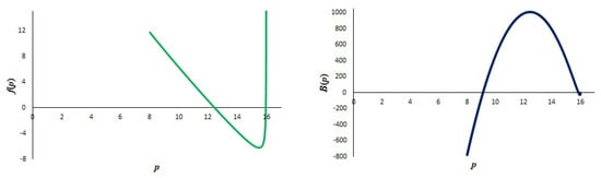
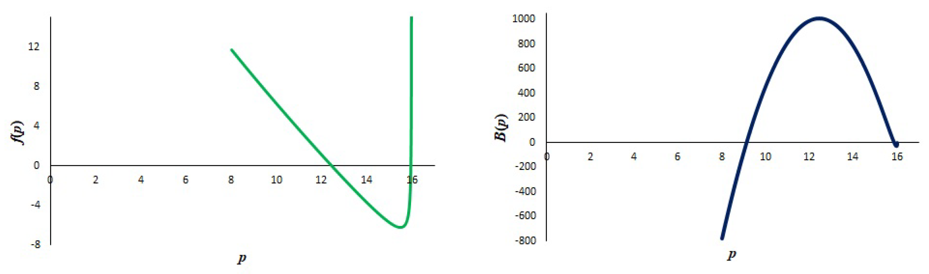
Suppose an inventory system for a single item with the same properties as those described in Section 2. Consider the following parameters: purchasing cost $c=\$8$ per unit, ordering cost $A=\$500$ per order, unit holding cost $h=\$2$ per unit and month, shortage cost $\pi =\$3.2$ per unit and month, and the index of the power demand pattern $n=2.5$. In addition, the demand rate per month is a function dependent on p which is fitted to the expression $D_2\left(p\right)=\alpha -\beta p^{\gamma }$, with the parameters $\alpha =1280$, $\beta =40$ and $\gamma =1.25$. Firstly, the maximum unit selling price $p_m=\$16$ per unit has to be calculated. Applying step 1 of Algorithm 1, we have $f^{\prime }\left(c\right)=-2.80766<0$. Next, the point $p_1={arg}_{p\in (8,16)}\{f^{\prime }\left(p\right)=0\}=15.5006$ is calculated. Also, $f\left(p_1\right)=-6.23179<0$ and, from step 5, we have $p_0={arg}_{p\in (8,p_1)}\{f\left(p\right)=0\}=12.4417$. As $B\left(p_0\right)=1005.97>0$, it is deduced that the optimum unit selling price is $p^{*}=p_0=\$12.4417$ per unit and the maximum profit is $B^{*}=B\left(p_0\right)=\$1005.97$ per month. From (13), the maximum inventory level is $S^{*}=538.721$ units and, from (14), the optimum inventory cycle is $T^{*}=1.89441$ months. Therefore, the economic lot size is $Q^{*}=654.192$ units. Figure 4 shows the functions $f\left(p\right)$ and $B\left(p\right)$ of this numerical example.

Figure 4. Functions $f\left(p\right)$ and $B\left(p\right)$ for Example 1.

Example 2.

Assume the same parameters as in Example 1, but now the values of c and α are changed to $c=\$6.25$ per unit and $\alpha =640$, respectively. Then the maximum unit selling price is $p_m=\$9.18959$ per unit. From step 1 of Algorithm 1, $f^{\prime }\left(c\right)=-2.47145$. From step 3, it follows that $p_1=8.66838$. As $f\left(p_1\right)=0.278539>0$, it can be concluded that, for any unit selling price, the inventory system cannot be profitable.

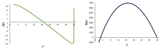
Example 3.

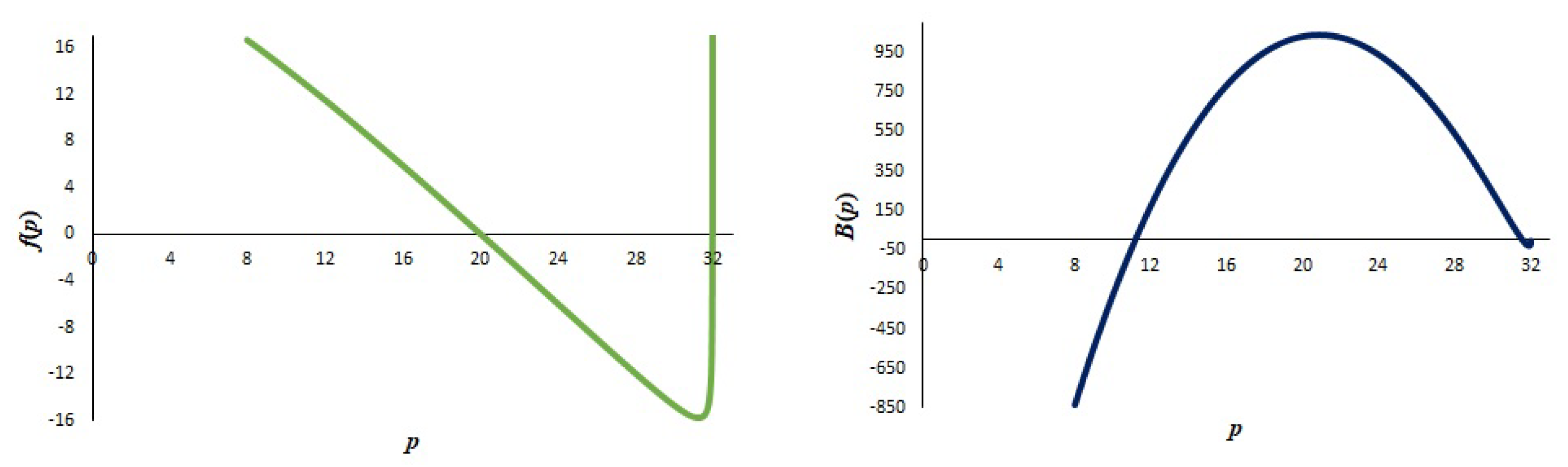
Assume the same parameters as Example 1, except for the values of β and γ. Now, assume that these parameters are $\beta =80$ and $\gamma =0.8$. The value of $p_m$ is now $p_m=\$32$ per unit. As $0<\gamma <1$, then the steps of Algorithm 2 are followed to find the optimal inventory policy. Thus, we have $f^{\prime }\left(c\right)=-1.18416<0$, $p_1={arg}_{p\in (8,32)}\{f^{\prime }\left(p\right)=0\}=31.2652$, $f\left(p_1\right)=15.6852$, $p_0={arg}_{p\in (8,p_1)}\{f\left(p\right)=0\}=20.0649$ and $B\left(p_0\right)=4245.02$. Consequently, the optimum unit selling price is $p^{*}=p_0=\$20.0649$ per unit, the inventory level is $S^{*}=578.982$ units, the inventory cycle is $T^{*}=1.76268$ months, the economic lot size is $Q^{*}=703.082$ units and the maximum profit per unit time is $B^{*}=\$4245.02$ per month. The functions $f\left(p\right)$ and $B\left(p\right)$ are shown in Figure 5.

Figure 5. Functions $f\left(p\right)$ and $B\left(p\right)$ for Example 3.

Algorithm 2  Obtaining the optimal policy and the maximum profit when $0<\gamma <1$
Step 1	Calculate $f^{\prime }\left(c\right)$ from (19).
	If $f^{\prime }\left(c\right)<0$, then go to step 6. Otherwise, go to step 2.
Step 2	From (20), obtain $f^{″}\left(c\right)$.
	If $f^{\prime }\left(c\right)\ge 0$, then go to step 8. Otherwise, go to step 3.
Step 3	Calculate $p_2={arg}_{p\in (c,p_m)}\{f^{″}\left(p\right)=0\}$.
	If $f^{\prime }\left(p_2\right)\ge 0$, then go to step 8. Otherwise, go to step 4.
Step 4	Calculate the points $p_3={arg}_{p\in (c,p_2)}\{f^{\prime }\left(p\right)=0\}$ and $p_4=$
	${arg}_{p\in (p_2,p_m)}\{f^{\prime }\left(p\right)=0\}$.
	If $f\left(p_4\right)\ge 0$, then go to step 8. Otherwise, go to step 5.
Step 5	Calculate $p_5={arg}_{p\in (p_1,p_4)}\{f\left(p\right)=0\}$.
	If $B\left(p_5\right)<0$, then go to step 8. Otherwise, take $p^{*}=p_5$ and go to step 9.
Step 6	Calculate $p_1={arg}_{p\in (c,p_m)}\{f^{\prime }\left(p\right)=0\}$.
	If $f\left(p_1\right)\ge 0$, then go to step 8. Otherwise, go to step 7.
Step 7	Calculate $p_0={arg}_{p\in (c,p_1)}\{f\left(p\right)=0\}$.
	If $B\left(p_0\right)<0$, then go to step 8. Otherwise, take $p^{*}=p_0$ and go to step 9.
Step 8	Set $p^{*}=p_m$. Put $B^{*}=0$, $S^{*}=0$ and $T^{*}=\infty$. Stop.
Step 9	From (13), calculate $S^{*}=S^{*}\left(p^{*}\right)$.
	From (14), calculate $T^{*}=T^{*}\left(p^{*}\right)$.
	From (15), determine $B^{*}=B\left(p^{*}\right)$. Stop.

Example 4.

Consider the same parameters as in Example 3, but changing the unit purchasing cost to $c=\$2$ per unit. Following Algorithm 2, we have $f^{\prime }\left(c\right)=0.0461332$, $f^{″}\left(c\right)=-0.735387$, $p_2=24.0160$, $f^{\prime }\left(p2\right)=-1.50313$, $p_3=2.06455$, $p_4=31.2652$, $f\left(p_4\right)=-20.4852$, $p_5=16.7939$ and $B\left(p_5\right)=6985.45$. Therefore, the optimal unit selling price is $p^{*}=p_5=\$16.7939$ per unit, the inventory level is $S^{*}=658.394$ units, the inventory cycle is $T^{*}=1.55008$ months, the economic lot size is $Q^{*}=799.517$ units and the profit per unit time is $B^{*}=\$6985.45$ per month. The functions $f\left(p\right)$ and $B\left(p\right)$ are plotted in Figure 6.

Figure 6. Functions $f\left(p\right)$ and $B\left(p\right)$ for Example 4.

Sensitivity Analysis

To analyze the effect of the parameters of the demand rate $\alpha$, $\beta$, $\gamma$ and n on the optimal policy and the maximum profit, three tables are presented where the evolution of the optimal policy $p^{*}$, $T^{*}$, $S^{*}$ and the maximum profit $B^{*}$ is shown for different values of $\alpha$, $\beta$, $\gamma$ and n. We assume the parameters $c=8$, $A=500$, $h=2$ and $\pi =3.2$. Table 2, Table 3 and Table 4 display computational results where $\alpha \in \{960,1280,1600\}$, $\beta \in \{36,40,44,48\}$, $\gamma \in \{0.8,0.9,1,1.1,1.2\}$ and $n\in \{0.5,1,2\}$. The obtained results can help us to identify some insights into the model presented in this paper. These characteristics are noted below:

Table 2. Sensitivity of the optimal policy $(p^{*},T^{*},S^{*})$ and the maximum profit $B^{*}$ to variations of the parameters $\alpha$, $\beta$ and $\gamma$ when $n=0.5$.

$\mathit{\gamma }$	$\mathit{\beta }$	$\mathit{\alpha }=960$				$\mathit{\alpha }=1280$				$\mathit{\alpha }=1600$
		${\mathit{p}}^{*}$	${\mathit{T}}^{*}$	${\mathit{S}}^{*}$	${\mathit{B}}^{*}$	${\mathit{p}}^{*}$	${\mathit{T}}^{*}$	${\mathit{S}}^{*}$	${\mathit{B}}^{*}$	${\mathit{p}}^{*}$	${\mathit{T}}^{*}$	${\mathit{S}}^{*}$	${\mathit{B}}^{*}$
$0.8$	36	33.9703	1.45619	196.207	8553.46	46.4856	1.22414	233.400	18,559.5	59.8418	1.07770	265.116	32,748.6
	40	30.3818	1.47661	193.493	7067.43	41.3443	1.23530	231.291	15,676.4	53.0474	1.08485	263.368	27,956.3
	44	27.5188	1.49838	190.682	5891.73	37.2418	1.24702	229.117	13,385.2	47.6258	1.09231	261.568	24,141.2
	48	25.1870	1.52160	187.772	4943.42	33.8999	1.25932	226.879	11,527.4	43.2094	1.10008	259.720	21,041.5
$0.9$	36	23.5002	1.48305	192.653	4642.68	30.5146	1.22897	232.483	10,432.9	37.7596	1.07359	266.129	18,548.4
	40	21.4261	1.51393	188.724	3759.01	27.6536	1.24552	229.393	8755.38	34.0919	1.08421	263.524	15,824.0
	44	19.7499	1.54726	184.659	3056.64	25.3395	1.26295	226.227	7409.87	31.1246	1.09525	260.866	13,631.0
	48	18.3692	1.58335	180.449	2488.97	23.4312	1.28132	222.984	6310.84	28.6771	1.10676	258.155	11,832.2
$1.0$	36	17.8440	1.54124	185.380	2477.78	22.1928	1.25233	228.146	6029.07	26.5811	1.08315	263.782	11,025.9
	40	16.5264	1.58864	179.849	1919.45	20.4230	1.27641	223.842	4969.40	24.3639	1.09831	260.140	9324.21
	44	15.4530	1.64129	174.079	1478.07	18.9769	1.30206	219.432	4116.89	22.5510	1.11418	256.435	7945.94
	48	14.5634	1.70034	168.033	1124.65	17.7739	1.32947	214.908	3419.84	21.0414	1.13081	252.664	6810.27
$1.1$	36	14.4814	1.64466	173.722	1199.80	17.3675	1.29742	220.218	3427.85	20.2414	1.10705	258.087	6632.63
	40	13.5922	1.72277	165.846	841.104	16.1880	1.33301	214.337	2726.39	18.7877	1.12860	253.159	5503.76
	44	12.8678	1.81504	157.415	563.855	15.2179	1.37185	208.269	2164.65	17.5896	1.15144	248.137	4588.56
	48	12.2713	1.92721	148.253	348.750	14.4066	1.41454	201.984	1708.73	16.5850	1.17573	243.010	3835.05
$1.2$	36	12.3573	1.83341	155.837	432.572	14.3471	1.37315	208.072	1811.40	16.3340	1.14852	248.767	3895.96
	40	11.7473	1.98802	143.718	212.329	13.5204	1.42881	199.967	1340.28	15.3235	1.17984	242.164	3121.70
	44	11.2706	2.20618	129.506	53.7066	12.8395	1.49242	191.444	969.265	14.4864	1.21383	235.382	2497.59
	48	12.1392	∞	0	0	12.2711	1.56645	182.396	674.862	13.7818	1.25100	228.389	1987.96

Table 3. Sensitivity of the optimal policy $(p^{*},T^{*},S^{*})$ and the maximum profit $B^{*}$ to variations of the parameters $\alpha$, $\beta$ and $\gamma$ when $n=1$.

$\mathit{\gamma }$	$\mathit{\beta }$	$\mathit{\alpha }=960$				$\mathit{\alpha }=1280$				$\mathit{\alpha }=1600$
		${\mathit{p}}^{*}$	${\mathit{T}}^{*}$	${\mathit{S}}^{*}$	${\mathit{B}}^{*}$	${\mathit{p}}^{*}$	${\mathit{T}}^{*}$	${\mathit{S}}^{*}$	${\mathit{B}}^{*}$	${\mathit{p}}^{*}$	${\mathit{T}}^{*}$	${\mathit{S}}^{*}$	${\mathit{B}}^{*}$
$0.8$	36	33.9511	1.51058	330.999	8578.45	46.4695	1.27008	393.676	18,589.2	59.8275	1.11822	447.139	32,782.3
	40	30.3624	1.53166	326.444	7092.07	41.3280	1.28161	390.134	15,705.9	53.0330	1.12562	444.200	27,989.8
	44	27.4991	1.55412	321.725	5916.01	37.2254	1.29372	386.481	13,414.4	47.6114	1.13334	441.175	24,174.5
	48	25.1671	1.57807	316.843	4967.34	33.8833	1.30643	382.722	11,556.3	43.1949	1.14137	438.070	21,074.6
$0.9$	36	23.4815	1.53804	325.089	4667.22	30.4991	1.27491	392.186	1.04625	37.7460	1.11386	448.889	18,582.3
	40	21.4069	1.56987	318.498	3783.04	27.6379	1.29200	386.997	8784.59	34.0782	1.12483	444.511	15,857.6
	44	19.7302	1.60420	311.683	3080.16	25.3236	1.31000	381.681	7438.68	31.1108	1.13625	440.044	13,664.2
	48	18.3491	1.64135	304.628	2511.96	23.4151	1.32895	376.237	6339.24	28.6632	1.14813	435.490	11,865.1
$1.0$	36	17.8249	1.59769	312.952	2501.40	22.1774	1.29886	384.953	6058.12	26.5680	1.12362	444.990	11,059.5
	40	16.5066	1.64643	303.688	1942.36	20.4073	1.32370	377.729	4997.91	24.3505	1.13929	438.872	9357.34
	44	15.4323	1.70050	294.032	1500.25	18.9609	1.35014	370.331	4144.84	22.5374	1.15567	432.650	7978.59
	48	14.5419	1.76104	283.924	1146.06	17.7575	1.37839	362.743	3447.21	21.0275	1.17283	426.318	6842.45
$1.1$	36	14.4610	1.70352	293.510	1221.94	17.3519	1.34516	371.704	3455.90	20.2282	1.14818	435.472	6665.50
	40	13.5704	1.78345	280.356	862.244	16.1719	1.38180	361.846	2753.69	18.7742	1.17041	427.199	5536.00
	44	12.8444	1.87758	266.300	583.928	15.2011	1.42175	351.680	2191.18	17.5757	1.19397	418.772	4620.16
	48	12.2457	1.99149	251.069	367.666	14.3892	1.46560	341.157	1734.46	16.5708	1.21901	410.170	3866.00
$1.2$	36	12.3337	1.89549	263.783	452.449	14.3305	1.42282	351.415	1837.91	16.3204	1.19081	419.881	3927.65
	40	11.7204	2.05175	243.694	230.677	13.5029	1.47992	337.857	1365.76	15.3094	1.22307	408.809	3152.54
	44	11.2384	2.26931	220.331	70.2684	12.8210	1.54503	323.618	993.668	14.4718	1.25804	397.443	2527.57
	48	12.1392	∞	0	0	12.2512	1.62061	308.526	698.120	13.7666	1.29624	385.731	2017.06

Table 4. Sensitivity of the optimal policy $(p^{*},T^{*},S^{*})$ and the maximum profit $B^{*}$ to variations of the parameters $\alpha$, $\beta$ and $\gamma$ when $n=2$.

$\mathit{\gamma }$	$\mathit{\beta }$	$\mathit{\alpha }=960$				$\mathit{\alpha }=1280$				$\mathit{\alpha }=1600$
		${\mathit{p}}^{*}$	${\mathit{T}}^{*}$	${\mathit{S}}^{*}$	${\mathit{B}}^{*}$	${\mathit{p}}^{*}$	${\mathit{T}}^{*}$	${\mathit{S}}^{*}$	${\mathit{B}}^{*}$	${\mathit{p}}^{*}$	${\mathit{T}}^{*}$	${\mathit{S}}^{*}$	${\mathit{B}}^{*}$
$0.8$	36	33.8825	1.74515	488.802	8668.27	46.4115	1.46819	581.010	18,696.0	59.7763	1.29299	659.737	32,903.6
	40	30.2930	1.76906	482.195	7180.67	41.2697	1.48133	575.856	15,811.7	52.9816	1.30144	655.453	28,110.4
	44	27.4287	1.79451	475.356	6003.34	37.1665	1.49512	570.543	13,519.2	47.5597	1.31025	651.045	24,294.2
	48	25.0957	1.82161	468.285	5053.36	33.8240	1.50959	565.078	11,660.1	43.1429	1.31942	646.519	21,193.5
$0.9$	36	23.4143	1.77522	480.524	4755.49	30.4435	1.47302	579.107	10,568.9	37.6974	1.28752	662.542	18,704.1
	40	21.3383	1.81114	470.992	3869.54	27.5816	1.49245	571.567	8889.63	34.0292	1.30003	656.165	15,978.2
	44	19.6600	1.84981	461.147	3164.82	25.2664	1.51288	563.848	7542.28	31.0613	1.31304	649.662	13,783.6
	48	18.2771	1.89155	450.971	2594.73	23.3571	1.53438	555.946	6441.37	28.6132	1.32658	643.032	11,983.3
$1.0$	36	17.7566	1.84122	463.298	2586.43	22.1225	1.49954	568.863	6162.63	26.5207	1.29817	657.106	11,180.3
	40	16.4358	1.89577	449.966	2024.91	20.3512	1.52766	558.393	5100.47	24.3026	1.31599	648.208	9476.45
	44	15.3588	1.95602	436.106	1580.22	18.9035	1.55754	547.680	4245.41	22.4887	1.33461	639.164	8096.03
	48	14.4651	2.02312	421.642	1223.33	17.6987	1.58939	536.706	3545.75	20.9780	1.35409	629.967	6958.18
$1.1$	36	14.3883	1.95765	435.743	1301.81	17.2950	1.55109	549.956	3556.87	20.1810	1.32558	643.515	6783.72
	40	13.4933	2.04565	416.998	938.604	16.1141	1.59230	535.725	2852.02	18.7259	1.35078	631.512	5651.99
	44	12.7618	2.14820	397.092	656.553	15.1413	1.63706	521.078	2286.78	17.5263	1.37742	619.298	4733.89
	48	12.1561	2.27045	375.711	436.260	14.3270	1.68599	505.954	1827.25	16.5201	1.40568	606.846	3977.42
$1.2$	36	12.2503	2.16454	394.094	524.458	14.2714	1.63717	521.041	1933.48	16.2720	1.37324	621.182	4041.70
	40	11.6267	2.32965	366.163	297.397	13.4407	1.70059	501.611	1457.70	15.2593	1.40955	605.179	3263.62
	44	11.1283	2.55028	334.486	130.916	12.7551	1.77238	481.292	1081.81	14.4199	1.44880	588.784	2635.60
	48	10.7404	2.87924	296.271	12.1444	12.1809	1.85491	459.878	782.244	13.7127	1.49151	571.927	2121.96

1.

When $\beta$, $\gamma$ and n are fixed, the optimal selling price $p^{*}$, the optimal maximum inventory level $S^{*}$ and the maximum profit per unit time $B^{*}$ increase as the parameter $\alpha$ increases. However, the optimal inventory cycle $T^{*}$ decreases as $\alpha$ increases.

2.

With fixed $\alpha$, $\gamma$ and n, if the value of $\beta$ is increasing, then there is a point $\widehat{\beta }$ such that $p^{*}\left(\beta \right)<p_m$ and $B\left(p^{*}\left(\beta \right)\right)>0$ for all $\beta <\widehat{\beta }$, and $p^{*}\left(\beta \right)=p_m$ and $B\left(p^{*}\left(\beta \right)\right)=0$ if $\beta \ge \widehat{\beta }$. Moreover, when $\beta <\widehat{\beta }$, the optimal unit selling price, the maximum inventory level and the optimal profit are all strictly decreasing as the parameter $\beta$ increases, while the optimal inventory cycle is strictly decreasing as the parameter $\beta$ increases.

3.

With fixed $\alpha$, $\beta$ and n, if the value of $\gamma$ is increasing, then there is a point $\widehat{\gamma }$ such that $p^{*}\left(\gamma \right)<p_m$ and $B\left(p^{*}\left(\gamma \right)\right)>0$ for all $\gamma <\widehat{\gamma }$, and $p^{*}\left(\gamma \right)=p_m$ and $B\left(p^{*}\left(\gamma \right)\right)=0$ if $\gamma \ge \widehat{\gamma }$. Moreover, when $\gamma <\widehat{\gamma }$, the optimal unit selling price, the maximum inventory level and the optimal profit are all strictly decreasing as the parameter $\gamma$ increases. However, the optimal inventory cycle is strictly decreasing as the parameter $\gamma$ increases.

4.

With fixed $\alpha$, $\beta$ and $\gamma$, if the index of the power demand pattern n is increasing, then there is a point $\widehat{n}$ such that $p^{*}\left(n\right)<p_m$ and $B\left(p^{*}\left(n\right)\right)>0$ for all $n>\widehat{n}$, and $p^{*}\left(n\right)=p_m$ and $B\left(p^{*}\left(n\right)\right)=0$ if $n<\widehat{n}$. Moreover, when $n>\widehat{n}$, the optimal unit selling price, the maximum inventory level and the optimal profit are all strictly decreasing as the parameter n increases. However, the optimal inventory cycle is strictly decreasing as the parameter n increases.

5.

The optimal inventory policy and the maximum unit selling price are not very sensitive to changes in the demand pattern index n. However, the optimal solution is quite sensitive to changes in the value of $\gamma .$

Next, we present some findings obtained from the sensitivity analysis. Thus, the modification of the parameter $\alpha$ associated with the price-dependent demand has a greater effect on the total profit per unit time in a positive way, more so than the variation of the sensibility parameter $\beta$ for the price-dependent demand. Therefore, the decision maker should boost the price-dependent demand by implementing policies that increase the parameter $\alpha$ of the demand rate (for example, applying some marketing policies such as quantity discount).

6. Conclusions

We have studied an inventory model where demand depends on time and the unit selling price. Shortages are allowed and completely backlogged. The objective is to maximize the profit per unit time, assuming that the profit is the difference between revenue obtained from product sales and the total inventory cost. This cost is the sum of the ordering, purchasing, holding and backordering costs.

We introduce an approach to determine the optimal inventory policy, the optimal selling-price and the maximum profit per unit time in all possible cases. In order to illustrate the theoretical results and the methodology developed for obtaining the optimal solution of the inventory problem, we have presented some numerical examples where the optimal inventory policies are determined following the steps described in the proposed algorithms.

To analyze the effect on the optimal policy of changes in the parameters associated with the demand rate, we present several computational results that allow us to carry out a sensitivity analysis of the inventory policy.

Future research lines related to this paper could be the following: (i) to study the inventory system for perishable items, considering the properties established in this paper; (ii) to analyze the same system assuming stochastic demand; and (iii) to consider partial backordering in the assumptions of the inventory system.

References

- Chung, K.J.; Lin, S.D.; Srivastava, H.M. The complete solution procedures for the mathematical analysis of some families of optimal inventory models with order-size dependent trade credit and deterministic and constant demand. Appl. Math. Comput. 2012, 219, 141–156. [Google Scholar] [CrossRef]
- Vandana; Sharma, B.K. An EOQ model for retailers partial permissible delay in payment linked to order quantity with shortages. Math. Comput. Simul. 2016, 125, 99–112. [Google Scholar] [CrossRef]
- Mokhtari, H. Economic order quantity for joint complementary and substitutable items. Math. Comput. Simul. 2018, 154, 34–47. [Google Scholar] [CrossRef]
- Lin, F.; Jia, T.; Wu, F.; Yang, Z. Impacts of two-stage deterioration on an integrated inventory model under trade credit and variable capacity utilization. Eur. J. Oper. Res. 2019, 272, 219–234. [Google Scholar] [CrossRef]
- Chung, K.J.; Liao, J.J.; Lin, S.D.; Chuang, S.T.; Srivastava, H.M. The inventory model for deteriorating items under conditions involving cash discount and trade credit. Mathematics 2019, 7, 596. [Google Scholar] [CrossRef] [Green Version]
- Khakzad, A.; Gholamian, M.R. The effect of inspection on deterioration rate: An inventory model for deteriorating items with advanced payment. J. Clean. Prod. 2020, 254, 120117. [Google Scholar] [CrossRef]
- Mishra, U.; Wu, J.Z.; Sarkar, B. A sustainable production-inventory model for a controllable carbon emissions rate under shortages. J. Clean. Prod. 2020, 256, 120268. [Google Scholar] [CrossRef]
- Naddor, E. Inventory Systems; John Wiley: New York, NY, USA, 1966. [Google Scholar]
- Datta, T.K.; Pal, A.K. Order level inventory system with power demand pattern for items with variable rate of deterioration. Indian J. Pure Appl. MatH. 1988, 19, 1043–1053. [Google Scholar]
- Lee, W.C.; Wu, J.W. An EOQ model for items with weibull distributed deterioration, shortages and power demand pattern. Int. J. Inform. Manag. Sci. 2002, 13, 19–34. [Google Scholar]
- Rajeswari, N.; Vanjikkodi, T. Deteriorating inventory model with power demand and partial backlogging. Int. J. Math. Arch. 2011, 2, 1495–1501. [Google Scholar]
- Mishra, S.; Raju, L.K.; Misra, U.K.; Misra, G. A study of EOQ model with power demand of deteriorating items under the influence of inflation. Gen. Math. Notes. 2012, 10, 41–50. [Google Scholar]
- Singh, D.P.; Kumar, S. A study of order level inventory system using power demand pattern for deteriorate items. Int. J. Eng. Math. Sci. 2012, 1, 178–184. [Google Scholar]
- Mishra, S.S.; Singh, P.K. Partial backlogging EOQ model for queued customers with power demand and quadratic deterioration: Computational approach. Am. J. Oper. Res. 2013, 3, 13–27. [Google Scholar]
- Rajeswari, N.; Indrani, K. EOQ policies for linearly time dependent deteriorating items with power demand and partial backlogging. Int. J. Math. Arch. 2015, 6, 122–130. [Google Scholar]
- Sicilia, J.; Febles-Acosta, J.; González-De la Rosa, M. Deterministic inventory systems with power demand pattern. Asia Pac. J. Oper. Res. 2012, 29, 1250025. [Google Scholar] [CrossRef]
- Sicilia, J.; Febles-Acosta, J.; González-De la Rosa, M. Economic order quantity for a power demand pattern system with deteriorating items. Eur. J. Ind. Eng. 2013, 7, 577–593. [Google Scholar] [CrossRef]
- San-José, L.A.; Sicilia, J.; González-De-la-Rosa, M.; Febles-Acosta, J. Optimal inventory policy under power demand pattern and partial backlogging. Appl. Math. Model. 2017, 46, 618–630. [Google Scholar] [CrossRef]
- Adaraniwon, A.O.; Omar, M.B. An inventory model for delayed deteriorating items with power demand considering shortages and lost sales. J. Intell. Fuzzy Syst. 2019, 36, 5397–5408. [Google Scholar] [CrossRef]
- Adaraniwon, A.O.; Omar, M.B. An inventory model for linearly time-dependent deteriorating rate and time-varying demand with shortages partially backlogged. J. Intell. Fuzzy Syst. 2020, 38, 4545–4557. [Google Scholar]
- San-José, L.A.; Sicilia, J.; Abdul-Jalbar, B. Optimal policy for an inventory system with demand dependent on price, time and frequency of advertisement. Comput. Oper. Res. 2021, 128, 105169. [Google Scholar] [CrossRef]
- Smith, N.R.; Martínez-Flores, J.L.; Cárdenas-Barrón, L.E. Analysis of the benefits of joint price and order quantity optimisation using a deterministic profit maximisation model. Prod. Plan. Control. 2007, 18, 310–318. [Google Scholar] [CrossRef]
- Soni, H.N. Optimal replenishment policies for non-instantaneous deteriorating items with price and stock sensitive demand under permissible delay in payment. Int. J. Prod. Econ. 2013, 146, 259–268. [Google Scholar] [CrossRef]
- Wu, J.; Skouri, K.; Teng, J.T.; Ouyang, L.Y. A note on “Optimal replenishment policies for non-instantaneous deteriorating items with price and stock sensitive demand under permissible delay in payment”. Int. J. Prod. Econ. 2014, 155, 324–329. [Google Scholar] [CrossRef]
- Avinadav, T.; Herbon, A.; Spiegel, U. Optimal ordering and pricing policy for demand functions that are separable into price and inventory age. Int. J. Prod. Econ. 2014, 155, 406–417. [Google Scholar] [CrossRef]
- San-José, L.A.; Sicilia, J.; González-De-la-Rosa, M.; Febles-Acosta, J. Best pricing and optimal policy for an inventory system under time-and-price-dependent demand and backordering. Ann. Oper. Res. 2020, 286, 351–369. [Google Scholar] [CrossRef]
- Pando, V.; San-José, L.A.; Sicilia, J.; Alcaide-López-de-Pablo, D. Profitability index maximization in an inventory model with a price- and stock-dependent demand rate in a power-form. Mathematics 2021, 9, 1157. [Google Scholar] [CrossRef]
- San-José, L.A.; García-Laguna, J. Optimal policy for an inventory system with backlogging and all-units discounts: Application to the composite lot size model. Eur. J. Oper. Res. 2009, 192, 808–823. [Google Scholar] [CrossRef]
- Birbil, Ş.İ.; Bülbül, K.; Frenk, J.B.G.; Mulder, H.M. On EOQ cost models with arbitrary purchase and transportation costs. J. Ind. Manag. Optim. 2015, 11, 1211–1245. [Google Scholar]
- Jakšič, M.; Fransoo, J.C. Optimal inventory management with supply backordering. Int. J. Prod. Econ. 2015, 159, 254–264. [Google Scholar] [CrossRef] [Green Version]
- Mishra, S.S.; Gupta, S.; Yadav, S.K.; Rawat, S. Optimization of fuzzified Economic Order Quantity model allowing shortage and deterioration with full backlogging. Am. J. Oper. Res. 2015, 5, 103–110. [Google Scholar]
- San-José, L.A.; Sicilia, J.; González-De-la-Rosa, M.; Febles-Acosta, J. Analysis of an inventory system with discrete scheduling period, time-dependent demand and backlogged shortages. Comput. Oper. Res. 2019, 109, 200–208. [Google Scholar] [CrossRef]
- Axsäter, S. Inventory Control; Springer: New York, NY, USA, 2000. [Google Scholar]
- Kunreuther, H.; Richard, J.F. Optimal pricing and inventory decisions for non-seasonal items. Econometrica 1971, 39, 173–175. [Google Scholar] [CrossRef]
- Kabirian, A. The economic production and pricing model with lot-size-dependent production cost. J. Glob. Optim. 2012, 54, 1–15. [Google Scholar] [CrossRef]
Publisher’s Note: MDPI stays neutral with regard to jurisdictional claims in published maps and institutional affiliations. |
© 2021 by the authors. Licensee MDPI, Basel, Switzerland. This article is an open access article distributed under the terms and conditions of the Creative Commons Attribution (CC BY) license (https://creativecommons.org/licenses/by/4.0/).