Approximating Solutions of Non-Linear Troesch’s Problem via an Efficient Quasi-Linearization Bessel Approach

Abstract

Two collocation-based methods utilizing the novel Bessel polynomials (with positive coefficients) are developed for solving the non-linear Troesch’s problem. In the first approach, by expressing the unknown solution and its second derivative in terms of the Bessel matrix form along with some collocation points, the governing equation transforms into a non-linear algebraic matrix equation. In the second approach, the technique of quasi-linearization is first employed to linearize the model problem and, then, the first collocation method is applied to the sequence of linearized equations iteratively. In the latter approach, we require to solve a linear algebraic matrix equation in each iteration. Moreover, the error analysis of the Bessel series solution is established. In the end, numerical simulations and computational results are provided to illustrate the utility and applicability of the presented collocation approaches. Numerical comparisons with some existing available methods are performed to validate our results.

1. Introduction

Mathematical modeling through differential equations is of great importance in different branches of science and engineering with their ability to provide more realistic simulations to real life phenomenons. The non-linear Troesch’s model problem has been used in the investigation of the theory of gas porous electrodes [1,2]. This model, as a two-point boundary value problem (BVP) has also found application in the confinement of a plasma column by radiation pressure [3]. To be more precise, the following two-point non-linear BVP is known as Troesch’s problem [4,5]

$${\psi }^{″}(\tau )=\alpha sinh(\alpha \psi (\tau )),$$

(1)

with the following boundary conditions

$$\psi (0)=0,\psi (1)=1.$$

(2)

Here, the constant parameter $\alpha$ is positive. In the closed-form, the exact solution of (1) has been obtained with the help of the elliptic function $\mathit{Sc}(·|·)$ of Jacobian type [6] in the form

$$\psi (\tau )=\frac{2}{\alpha }{sinh}^{-1}\left[\frac{{\psi }^{\prime }(0)}{2}\mathit{Sc}(\alpha \tau |1-\frac{1}{4}{({\psi }^{\prime }(0))}^2)\right].$$

(3)

Here, the derivative of $\psi$ at 0 is given by ${\psi }^{\prime }(0)=2{(1-x)}^{\frac{1}{2}}$ such that x is the solution of the transcendental equation $sinh(\frac{\alpha }{2})={(1-x)}^{\frac{1}{2}}\mathit{Sc}(\alpha |x)$. The elliptic function $\mathit{Sc}(\alpha |x)$ is defined as $\mathit{Sc}(\alpha |x)=\frac{sin\beta }{cos\beta }$, where $\beta$ and $\alpha$ are related through the integral representation $\alpha ={\int }_0^{\beta }\frac{dt}{1-x{sin}^{2}t}$. For $\alpha >1$,  Troesch’s problem is known to be an unstable two-point BVP due to existence of a pole, which is located approximately at ${\tau }_s=ln(8/{\psi }^{\prime }(0))/\alpha$ [4]. These singularities hinder most of the numerical methods to capture the solutions of the Troesch’s problem, especially for large values of the parameter $\alpha$.

Over the past decades, a considerable attention has been drawn to the numerical solutions of (1). Among other existing approaches, let us mention the following methods: the shooting schemes [5,6,7,8,9], the embedding technique [10], the combined approach based on modified decomposition and Laplace transform [11], the modified homotopy perturbation algorithm [12], the finite element method based on B-splines [13], the sinc-Galerkin methods [14,15], the discontinuous Galerkin finite element scheme [16], the stochastic algorithm based on artificial neural network [17], the shifted Jacobi–Gauss collocation scheme [18], the finite difference scheme based on a Shishkin mesh [19], the shifted Bessel Tau method [20], the iterative method based on Green’s function and optimal homotopy analysis technique [21], the one-step hybrid block method [22], and the wavelet-homotopy analysis method [23].

In this manuscript, an efficient and reliable method based on the quasi-linearization technique combined with Bessel functions is proposed to obtain an accurate approximate series solution of Troesch’s model problem (1). Additionally, the direct Bessel collocation approach is also developed for this model problem. In the former method, we solve the original model via converting it into a sequence of linearized subproblems in conjunction with an iteration parameter r, which will be set at most 5. In the latter approach, we solve it directly via the Bessel matrix algorithm, which converts the governing differential equation into a system of non-linear algebraic equations. The Bessel polynomials first appeared in the study of the solution of classical wave equation and were systematically introduced in [24]. However, they are recently adapted to solve differential equations through a collocation procedure [25,26,27,28]. The main feature of the novel Bessel polynomials is that all coefficients are positive integers. It is also worth mentioning that the Bessel functions used here are different from the Bessel functions of the first kind, which were previously considered in the literature, see cf. [29,30,31,32]. Collocation-based approaches along with (orthogonal) basis functions are very common in solving differential and integral equations due to their simplicity and efficiency. Among many different bases used in the literature, let us consider the methods based on the Legendre, Chebyshev, Jacobi, Genocchi, and Hermit functions reported in [33,34,35,36,37,38].

The rest of this paper is organized as follows: in Section 2, a brief discussion on the Bessel polynomials is given. Hence, the technique of quasi-linearization for the model problem is discussed. Section 3 is devoted to the methodology of the direct Bessel-collocation procedure for the Troesch model problem. Converting the boundary conditions into a matrix form is also done afterwards. The second and efficient Bessel collocation approach based on the quasi-linearlization technique is given in Section 4. An error analysis of the Bessel solution is given in Section 5. Numerical experiments and discussions of the presented methods are reported in Section 6. Finally, a conclusion is made in the last section.

2. Basic Facts

2.1. Bessel Functions

Let us assume that k is a positive integer. The Bessel polynomials are known to be the solutions of the following second-order differential equation

$${\tau }^2{y}^{″}(\tau )+(2\tau +2)y^{\prime }(\tau )=k(k+1)y(\tau ),$$

(4)

which has naturally appeared in the study of classical wave equation [24], see also [25]. The first two Bessel polynomials are ${\mathit{B}}_0(\tau )=1$ and ${\mathit{B}}_1(\tau )=1+\tau$. The remaining Bessel polynomials can be determined via the following recurrence formula

$${\mathit{B}}_{k+1}(\tau )={\mathit{B}}_{k-1}(\tau )+(2k+1)\tau {\mathit{B}}_k(\tau ),k=1,2,\dots .$$

(5)

In an explicit form, we can write these polynomials as

$${\mathit{B}}_k(\tau )=\sum _{\ell =0}^k\frac{(k+\ell )!}{2^{\ell }\ell !(k-\ell )!}{\tau }^{\ell },k=0,1,\dots .$$

(6)

Obviously, all coefficients of each ${\mathit{B}}_k(\tau )$ are positive and the constant term for each one is 1. It can be proved that the set of these polynomials forms an orthogonal system on the unit circle. The corresponding weighting function is $\omega (\tau )=e^{-\frac{2}{\tau }}$.

The key of the presented method is that the unknown solution $\psi (\tau )$ and its second-order derivative in (1) are expressed in terms of a truncated series of Bessel polynomials with expansion coefficients as

$${\psi }_M(\tau )=\sum _{k=0}^M{d}_k{\mathit{B}}_k(\tau ),0\le \tau \le 1.$$

(7)

Hence, our aim will be reduced to find the expansion coefficients $d_k$ for $k=0,1,\dots ,M$. Let us introduce the vector of unknown as $D_M={[d_0{d}_1\dots d_M]}^t$. Thus, we may write the relation (7) in the following representation form

$${\psi }_M(\tau )={\mathbf{\Omega }}_M(\tau )D_M,$$

(8)

being ${\mathbf{\Omega }}_M(\tau )$ the vector of Bessel basis defined as

$${\mathbf{\Omega }}_M(\tau )=\left[{\mathit{B}}_0(\tau ){\mathit{B}}_1(\tau )\dots {\mathit{B}}_M(\tau )\right].$$

It can be easily shown that ${\mathbf{\Omega }}_M(\tau )$ in (8) is expressed as a product of the monomial basis functions with a lower-triangular matrix as

$${\mathbf{\Omega }}_M(\tau )={\mathbf{\Pi }}_M(\tau )C^t,$$

(9)

where ${\mathbf{\Pi }}_M(\tau )=\left[1\tau {\tau }^2\dots {\tau }^M\right]$ and $\mathit{C}$ can be represented as

$$C^t={\left(\begin{array}{cccccc}1& 1& 1& \dots & 1& 1\\ 0& 1& 3& \dots & \frac{M!}{2(M-2)!1!}& \frac{(M+1)!}{2(M-1)!1!}\\ 0& 0& 3& \dots & \frac{(M+1)!}{2^2(M-3)!2!}& \frac{(M+2)!}{2^2(M-2)!2!}\\ ⋮& ⋮& \ddots & \ddots & \ddots & ⋮\\ 0& 0& 0& \dots & \frac{(2M-2)!}{2^{M-1}0!(M-1)!}& \frac{(2M-1)!}{2^{M-1}1!(M-1)!}\\ 0& 0& 0& \dots & 0& \frac{(2M)!}{2^{M}0!M!}\end{array}\right)}_{(M+1)\times (M+1)}.$$

By utilizing (8) and (9), we may represent the approximated solution ${\psi }_M(\tau )$ in (7) as follows

$${\psi }_M(\tau )={\mathbf{\Omega }}_M(\tau )D_M={\mathbf{\Pi }}_M(\tau )C^t{D}_M.$$

(10)

2.2. Quasi-Linearization Approach

The technique of quasi-lineraization aims to transform the original model problem (1) into a sequence of linear equations. Afterwards, we will apply the Bessel collocation procedure to the resultant linearized models. In this respect, the basic ideas underlying the solutions of our model problems via quasi-linearization method (QLM) are briefly described, see [39,40,41] for more detailed discussions and applications.

By defining

$$G(\tau ,\psi ):=\alpha sinh(\alpha \psi (\tau )),$$

one can rewrite the general form of our model problem (1) as

$${\psi }^{″}(\tau )=G(\tau ,\psi ),\tau \in [0,1].$$

(11)

The non-linear form (11) will also be accompanied with the boundary conditions (2). Let assume that the initial approximation ${\psi }_0(\tau )$ to the solution $\psi (\tau )$ of (1) is given. Hence, the QLM iteration for (11) is defined as

$${\psi }_{r+1}^{″}(\tau )=G(\tau ,{\psi }_r) + \left({\psi }_{r+1}(\tau )-{\psi }_r(\tau )\right)G_{\psi }(\tau ,{\psi }_r),$$

for $r=0,1,\dots$ and with the same boundary conditions as given in (2). Here, $G_{\psi }$ is the functional derivative of $G(\tau ,\psi )$ with respect to $\psi$. By applying the QLM technique on the non-linear model problem (1), the following linearized model form is obtained

$$\begin{array}{c}\hfill {\psi }_{r+1}^{\prime \prime }(\tau )-\left[{\alpha }^{2}cosh(\alpha {\psi }_r(\tau ))\right]{\psi }_{r+1}(\tau )=-{\alpha }^2{\psi }_r(\tau )cosh(\alpha {\psi }_r(\tau ))+\alpha sinh(\alpha {\psi }_r(\tau )),\end{array}$$

(12)

for $r=0,1,\dots$. To each lineraized equation, the following boundary conditions are supplemented

$$\begin{array}{c}\hfill {\psi }_{r+1}(0)=0,{\psi }_{r+1}(1)=1.\end{array}$$

(13)

Consequently, we solve the quasilinear model problem (12) together with boundary conditions (13) via the Bessel collocation approach rather than applying it to the original Equation (1) directly. The latter approach is referred to as the QLM-Bessel.

3. Direct Approach

To proceed, we partition the domain $[0,1]$ uniformly into M subdomains. Below, the following collocation points are used

$${\tau }_i=\frac{i}{M},i=0,1,\dots ,M.$$

(14)

We next substitute the collocation points (14) into (10), we arrive at

$$\mathbf{\Psi }=\mathbf{\Delta }{\mathit{C}}^t{\mathit{D}}_M,\mathbf{\Delta }=\left(\begin{array}{c}{\mathbf{\Pi }}_M({\tau }_0)\\ {\mathbf{\Pi }}_M({\tau }_1)\\ ⋮\\ {\mathbf{\Pi }}_M({\tau }_M)\end{array}\right),\mathbf{\Psi }=\left(\begin{array}{c}{\psi }_M({\tau }_0)\\ {\psi }_M({\tau }_1)\\ ⋮\\ {\psi }_M({\tau }_M)\end{array}\right).$$

(15)

Our next aim is to represent the second-order derivatives of $\psi (\tau )$ at the collocation points in a matrix representation form. For this purpose, we need to calculate $\frac{d^2}{d{\tau }^2}{\mathbf{\Pi }}_M(\tau )$. It can be easily checked that

$$\begin{array}{c}\hfill \frac{d}{d\tau }{\mathbf{\Pi }}_M(\tau )={\mathbf{\Pi }}_M(\tau )E^t,\end{array}$$

(16)

where the matrix $\mathit{E}$ denotes the operational matrix of differentiation and is defined as

$${\mathit{E}}^t={\left(\begin{array}{ccccc}0& 1& 0& \dots & 0\\ 0& 0& 2& \dots & 0\\ ⋮& ⋮& 0& ⋮& ⋮\\ 0& 0& 0& \ddots & M\\ 0& 0& 0& \dots & 0\end{array}\right)}_{(M+1)\times (M+1)}.$$

By applying differentiation on (16), we obtain

$$\begin{array}{c}\hfill \frac{d^2}{d{\tau }^2}{\mathbf{\Pi }}_M(\tau )={\mathbf{\Pi }}_M(\tau ){(E^t)}^2.\end{array}$$

(17)

Lemma 1.

The matrix representation form of$\frac{d^2}{d{\tau }^2}{\psi }_M(\tau )$at the collocation points (14) is given by

$${\mathbf{\Psi }}^{(2)}=\mathbf{\Delta }{(E^t)}^2{C}^t{D}_M,$$

(18)

where the matrix $\mathit{E}$ and the vector $\mathsf{\Delta }$ are defined in (16) and (15), respectively, and

$${\mathbf{\Psi }}^{(2)}=\left(\begin{array}{c}{\psi }_M^{″}({\tau }_0)\\ {\psi }_M^{″}({\tau }_1)\\ ⋮\\ {\psi }_M^{″}({\tau }_M)\end{array}\right).$$

Proof. 

We differentiate (10) two times with respect to $\tau$ to obtain

$$\frac{d^2}{d{\tau }^2}{\psi }_M(\tau )=\frac{d^2}{d{\tau }^2}{\mathbf{\Pi }}_M(\tau )C^t{D}_M.$$

(19)

We combine relations (17) and (19) to obtain

$$\frac{d^2}{d{\tau }^2}{\psi }_M(\tau )={\mathbf{\Pi }}_M(\tau ){(E^t)}^2{C}^t{D}_M.$$

(20)

Now, it is sufficient to insert the collocation points (14) into (20). By considering the definitions of $\mathbf{\Delta }$ and ${\mathbf{\Psi }}^{(2)}$ the proof is concluded.    □

We now proceed by placing the collocation points (14) into the model problem to obtain

$$\frac{d^2}{d{\tau }^2}{\psi }_M({\tau }_i)-\alpha sinh(\alpha {\psi }_M({\tau }_i))=0,i=0,1,\dots ,M.$$

(21)

In the matrix notation form, we are able to write the preceding equations as

$${\mathbf{\Psi }}^{(2)}+\mathbf{A}\hat{\mathbf{\Psi }}=\mathit{Z}.$$

(22)

where the matrix $\mathit{A}$ and the right-hand-side vector $\mathit{Z}$ are

$$\mathit{A}=\left(\begin{array}{cccc}\alpha & 0& \dots & 0\\ 0& \alpha \dots & 0\\ ⋮& ⋮& \ddots & ⋮\\ 0& 0& \dots & \alpha \end{array}\right),\mathit{Z}=\left(\begin{array}{c}0\\ 0\\ ⋮\\ 0\end{array}\right),$$

and the matrix $\hat{\mathbf{\Psi }}$ takes the form $sinh(-\mathit{A}\mathbf{\Psi })$ or, equivalently, $\hat{\mathbf{\Psi }}=\frac{1}{2}(e^{-\mathit{A}\mathbf{\Psi }}-e^{\mathit{A}\mathbf{\Psi }})$.

Suppose that the approximate solution of (1) can be written as (7) or (10). By placing the relations (15) and (18) into (22), we obtain the following fundamental matrix equation

$$\underset{\mathbf{\Sigma }}{\underbrace{\mathbf{\Delta }{(E^t)}^2{\mathit{C}}^t{D}_M+\mathit{A}sinh\left(-\mathit{A}\mathbf{\Delta }{\mathit{C}}^t{\mathit{D}}_M\right)}}=\mathit{Z},\mathrm{or}[\mathbf{\Sigma };\mathit{Z}].$$

(23)

It can be clearly seen that the relation (23) is a non-linear matrix equation, which can be solved for the vector of unknowns ${\mathit{D}}_M$ as the Bessel coefficients by using, e.g., Newton-type solvers. However, we are left with the task of entering the boundary conditions (2) into the fundamental matrix equation.

Boundary Conditions in the Matrix Forms

To obtain the approximated solution of our model problem (1) by solving the fundamental matrix Equation (23), we need to take into account the boundary conditions (2). First, we consider the initial condition $\psi (0)=0$. For this purpose, we let $\tau \to 0$ in (10) to obtain

$${\hat{\mathbf{\Sigma }}}_0:={\mathbf{\Pi }}_M(0)C^t{D}_M=0,\mathrm{or}[{\hat{\mathbf{\Sigma }}}_0;0].$$

For the end condition $\psi (1)=1$, we tend $\tau \to 1$ in (10) to arrive at

$${\hat{\mathbf{\Sigma }}}_1:={\mathbf{\Pi }}_M(1)C^t{D}_M=1,\mathrm{or}[{\hat{\mathbf{\Sigma }}}_1;1].$$

Remark 1.

We note that the computational complexity of evaluating$\frac{d^2}{d{\tau }^2}{\mathbf{\Pi }}_M(\tau )$at the collocation points via (17) is on the order $\mathcal{O}({(M+1)}^2)$. In the following, we propose an alternative to reduce the involved complexity within $\mathcal{O}(M+1)$. The following algorithm will be invoked to calculate the second-order derivative of the basis functions ${\mathbf{\Pi }}_M(\tau )$ directly. Indeed, Algorithm 1 takes ${\mathbf{\Pi }}_M(\tau )$ as input and the output is ${\mathbf{\Pi }}_M^{(s)}(\tau )$ for $s=1,2,\dots$. For instance, by calling Algorithm 1 with $s=2$ and $M=5$, we obtain

$$\begin{array}{c}\hfill {\mathbf{\Pi }}_5^{(2)}(\tau )=\left[0026\tau 12{\tau }^{2}20{\tau }^3\right].\end{array}$$

Algorithm 1 The computation of s-derivative of the vector ${\mathbf{\Pi }}_M(\tau )$

procedure$[{\mathbf{\Pi }}_M^{(s)}]$= compute_DerPro$(M,s)$ ${\mathbf{\Pi }}_M^{(s)}[1]:=0$; for$j:=1,\dots ,M$do  if ($j-s<0$) then   ${\mathbf{\Pi }}_M^{(s)}[j+1]:=0$;  else   ${\displaystyle {\mathbf{\Pi }}_M^{(s)}[j+1]:=\frac{j!}{(j-s)!}{\tau }^{j-s}}$; end;

We are now able to enter the boundary conditions (2) into the fundamental matrix Equation (23). In this respect, we replace the first row as well as the last row of the augmented matrix $[\mathbf{\Sigma };\mathit{Z}]$ in (23) by the row matrices $[{\hat{\mathbf{\Sigma }}}_0;0]$ and $[{\hat{\mathbf{\Sigma }}}_1;1]$. Therefore, the resultant modified fundamental matrix becomes $[\hat{\mathbf{\Sigma }};\hat{\mathit{Z}}]$. After solving this modified matrix equation, the unknown coefficients $d_k$, $k=0,1,\dots ,M$ will be computed and, therefore, the approximate solution ${\psi }_M(\tau )$ for the model problem in (1) will be determined.

4. QLM-Bessel

Our goal is to solve the two-point BVP (1)–(2) approximately such that the desired solution is represented in terms of the truncated Bessel series (10). Unlike the direct Bessel-collocation approach described in the last section, this task is accomplished for the corresponding approximated quasilinear model problem (12). For this purpose, let us assume that an approximated solution ${\psi }_M^{(r)}(\tau )$ is known for the model problems (12) in the iteration $r=0,1,\dots$. In the next iteration, we consider

$${\psi }_M^{(r+1)}(\tau )=\sum _{k=0}^M{d}_k^{(r)}{\mathit{B}}_k(\tau ),0\le \tau \le 1.$$

(24)

Here, $d_k^{(r)}$, $k=0,1,\dots ,M$ are the unknown coefficients that have to be sought. Let us define

$$D_M^{(r)}={\left[d_0^{(r)}{d}_1^{(r)}\dots d_M^{(r)}\right]}^t.$$

Utilizing (10), we can rewrite the finite series (24) in a matrix representation form

$${\psi }_M^{(r+1)}(\tau )={\mathbf{\Pi }}_M(\tau ){\mathit{C}}^t{D}_M^{(r)},$$

(25)

where the vector of basis function ${\mathbf{\Pi }}_M(\tau )$ and the matrix $\mathit{C}$ are defined in (9). Calling Algorithm 1, we calculate the second-order derivative of the vector of basis functions ${\mathbf{\Pi }}_M(\tau )$ as

$$\frac{d^2}{d{\tau }^2}{\psi }_M^{(r+1)}(\tau )={\mathbf{\Pi }}_M^{(2)}(\tau ){\mathit{C}}^t{D}_M^{(r)}={\mathbf{\Pi }}_M(\tau ){({\mathit{E}}^t)}^2{\mathit{C}}^t{D}_M^{(r)}.$$

(26)

We then proceed by placing the collocation points (14) into (25) and (26) to write

$$\begin{array}{cccc}\hfill & {\mathbf{\Psi }}_{r+1}=\mathbf{\Delta }{\mathit{C}}^t{\mathit{D}}_M^{(r)},\hfill & \hfill {\mathbf{\Psi }}_{r+1}=\left(\begin{array}{c}{\psi }_M^{(r+1)}({\tau }_0)\\ {\psi }_M^{(r+1)}({\tau }_1)\\ ⋮\\ {\psi }_M^{(r+1)}({\tau }_M)\end{array}\right),& \mathbf{\Delta }=\left(\begin{array}{c}{\mathbf{\Pi }}_M({\tau }_0)\\ {\mathbf{\Pi }}_M({\tau }_1)\\ ⋮\\ {\mathbf{\Pi }}_M({\tau }_M)\end{array}\right),\hfill \end{array}$$

(27)

$$\begin{array}{ccc}\hfill & {\ddot{\mathbf{\Psi }}}_{r+1}=\mathbf{\Delta }{(E^t)}^2{\mathit{C}}^t{\mathit{D}}_M^{(r)},\hfill & \hfill {\ddot{\mathbf{\Psi }}}_{r+1}=\left(\begin{array}{c}\frac{d^2}{d{\tau }^2}{\psi }_M^{(r+1)}({\tau }_0)\\ \frac{d^2}{d{\tau }^2}{\psi }_M^{(r+1)}({\tau }_1)\\ ⋮\\ \frac{d^2}{d{\tau }^2}{\psi }_M^{(r+1)}({\tau }_M)\end{array}\right).\end{array}$$

(28)

We now are aiming to find an approximate solution represented as (24) for the quasilinear model problem (12) through the Bessel-collocation approach. By collocating (12) at the collocation points (14), we obtain

$${\psi }_{r+1}^{″}({\tau }_i)-\left[{\alpha }^{2}cosh(\alpha {\psi }_r({\tau }_i))\right]{\psi }_{r+1}({\tau }_i)=-{\alpha }^2{\psi }_r({\tau }_i)cosh(\alpha {\psi }_r({\tau }_i))+\alpha sinh(\alpha {\psi }_r({\tau }_i)),$$

for $r=0,1,\dots$. To proceed, we define

$$p_r(t)=-{\alpha }^{2}cosh(\alpha {\psi }_r(t)),f_r(t)=p_r(t){\psi }_r(t)+\alpha sinh(\alpha {\psi }_r(t)).$$

Now, by using the matrix notations defined in (27) and (28), we may write the preceding equations as compactly as

$${\ddot{\mathbf{\Psi }}}_{r+1}+{\mathit{P}}_r{\mathbf{\Psi }}_{r+1}={\mathit{F}}_r.$$

(29)

In (29), the matrix ${\mathit{P}}_r$ as well as the vector ${\mathit{F}}_r$ can be written in the following forms

$${\mathit{P}}_r={\left(\begin{array}{cccc}{p}_r({\tau }_0)& 0& \dots & 0\\ 0& p_r({\tau }_1)& \dots & 0\\ ⋮& ⋮& \ddots & ⋮\\ 0& 0& \dots & p_r({\tau }_M)\end{array}\right)}_{(M+1)\times (M+1)},{\mathit{F}}_r={\left(\begin{array}{c}{f}_r({\tau }_0)\\ f_r({\tau }_1)\\ ⋮\\ f_r({\tau }_M)\end{array}\right)}_{(M+1)\times 1}.$$

Lemma 2.

Suppose that the approximate solution of (12) can be written as (25). Then, we obtain the following fundamental linear matrix equation

$$\underset{{\mathbf{\Sigma }}_r}{\underbrace{\left(\mathbf{\Delta }{({\mathit{E}}^t)}^2+{\mathit{P}}_r\mathbf{\Delta }\right){\mathit{C}}^t}}{D}_M^{(r)}={\mathit{F}}_r,\mathrm{or}[{\mathbf{\Sigma }}_r;{\mathit{F}}_r].$$

(30)

Proof. 

By inserting the relations (27) and (28) into (29), we obtain the fundamental matrix equation as desired. □

It can be obviously seen that, unlike Equation (22), the fundamental matrix equation (30) is a set of $(M+1)$ linear equations in terms of $(M+1)$ unknown coefficients $d_0^{(r)},d_1^{(r)},\dots ,d_M^{(r)}$ to be determined. In each iteration, one requires to take into consideration the boundary conditions (13). The matrix representations of the boundary conditions (13) can be similarly done as for the non-linear counterpart. Besides, to begin the computation, we need to prescribe the initial guess ${\psi }_0(\tau )$ as an approximation for the solution.

In a similar manner as the direct approach, the first and last rows of the augmented matrix $[{\mathbf{\Sigma }}_r;{\mathit{F}}_r]$ are replaced by the row matrices $[{\hat{\mathbf{\Sigma }}}_{r,0};0]$ and $[{\hat{\mathbf{\Sigma }}}_{r,1};1]$. The resulting algebraic system of linear equations becomes

$${\hat{\mathbf{\Sigma }}}_r{D}_M^{(r)}={\hat{\mathit{F}}}_r,$$

(31)

which can be solved by any classical linear solver. Consequently, the unknown Bessel coefficients in (24) will be determined once we solve this system of equations.

5. Error Analysis

In this section, we make an investigation on error analysis for the Bessel series solution. In this respect, we present a theorem giving an upper boundary of errors.

Theorem 1

(Upper Boundary of Errors). Let $\psi (\tau )$ and ${\psi }_M(\tau )={\mathbf{\Omega }}_M(\tau ){\mathit{D}}_M$ be the exact solution and the Bessel polynomial solution with M-th degree of (1). In addition, we assume that ${\psi }_M^{Mac}(\tau )={\mathbf{\Pi }}_M(\tau ){\tilde{D}}_M$ is the expansion of the Maclaurin series by M-th degree of $\psi (\tau )$. Then, the error of the Bessel polynomial solution is bounded as follows

$$\parallel \psi (\tau )-{\psi }_M{(\tau )\parallel }_{\infty }\le \parallel \stackrel{\infty }{\sum _{m=M+1}}\frac{{\psi }^{(m)}(0)}{m!}{\tau }^m{\parallel }_{\infty }+ \parallel {\tilde{\mathit{D}}}_M{\parallel }_{\infty }+\parallel C_M^t{\parallel }_{\infty }{\parallel D_M\parallel }_{\infty },$$

(32)

where ${\mathbf{\Pi }}_M(\tau )=\left[1\tau {\tau }^2\dots {\tau }^M\right]$, ${\mathbf{\Omega }}_M(\tau )=\left[{\mathit{B}}_0(\tau ){\mathit{B}}_1(\tau )\dots {\mathit{B}}_M(\tau )\right]$ and the matrix $C_M^t$ represents the coefficient matrix $C^t$ of size $(M+1)\times (M+1)$ as defined in the Section 2.

Proof. 

Utilizing the triangle inequality after adding and subtracting the Maclaurin expansion ${\psi }_M^{Mac}(\tau )$ by M-th degree, we write the following expression

$$\begin{array}{cc}\hfill \parallel \psi (\tau )-{\psi }_M{(\tau )\parallel }_{\infty }& =\parallel \psi (\tau )-{\psi }_M^{Mac}(\tau )+{\psi }_M^{Mac}(\tau )-{\psi }_M{(\tau )\parallel }_{\infty }\hfill \\ \hfill & \le \parallel \psi (\tau )-{\psi }_M^{Mac}{(\tau )\parallel }_{\infty }+{\parallel {\psi }_M^{Mac}(\tau )-{\psi }_M(\tau )\parallel }_{\infty }.\hfill \end{array}$$

(33)

According to (10), the Bessel polynomial solution ${\psi }_M(\tau )={\mathbf{\Omega }}_M(\tau )D_M$ can be written in the matrix form ${\psi }_M(\tau )={\mathbf{\Pi }}_M(\tau )C_M^t{D}_M$. Since the expansion of the Maclaurin series of $\psi (\tau )$ by M-th degree is ${\psi }_M^{Mac}(\tau )={\mathbf{\Pi }}_M(\tau ){\tilde{\mathit{D}}}_M$, we can write

$$\begin{array}{cc}\hfill \parallel {\psi }_M^{Mac}(\tau )-{\psi }_M{(\tau )\parallel }_{\infty }& =\parallel {\mathbf{\Pi }}_M(\tau ){\tilde{D}}_M-{\mathbf{\Pi }}_M(\tau ){\mathit{C}}_M^t{\mathit{D}}_M{\parallel }_{\infty }\hfill \\ \hfill & \le \parallel {\mathbf{\Pi }}_M{(\tau )\parallel }_{\infty }\left(\parallel {\tilde{\mathit{D}}}_M{\parallel }_{\infty }+\parallel {\mathit{C}}_M^t{\parallel }_{\infty }{\parallel {\mathit{D}}_M\parallel }_{\infty }\right).\hfill \end{array}$$

(34)

Due to the fact that $\parallel {\mathbf{\Pi }}_M{(\tau )\parallel }_{\infty }\le 1$ for $\tau \in [0,1]$, we can arrange Equation (34) as follows

$$\parallel {\psi }_M^{Mac}(\tau )-{\psi }_M{(\tau )\parallel }_{\infty }\le \parallel {\tilde{\mathit{D}}}_M{\parallel }_{\infty }+\parallel C_M^t{\parallel }_{\infty }{\parallel D_M\parallel }_{\infty }.$$

(35)

On the other hand, since the remainder term of the Maclaurin series ${\psi }_M^{Mac}(\tau )$ by M-th degree is ${\displaystyle \sum _{m=M+1}^{\infty }}\frac{{\psi }^{(m)}(0)}{m!}{\tau }^m,$$\frac{{\psi }^{(m)}(0)}{m!}{\tau }^m,$ we can write

$$\parallel \psi (\tau )-{\psi }_M^{Mac}{(\tau )\parallel }_{\infty }\le \parallel \stackrel{\infty }{\sum _{m=M+1}}\frac{{\psi }^{(m)}(0)}{m!}{\tau }^m{\parallel }_{\infty }.$$

(36)

Combining Equations (33), (35), and (36), the proof of the theorem is completed. □

Remark 2.

The upper bound obtained in Theorem 1 can be slightly modified. In fact, according to the remainder of the Taylor’s theorem, there exist$c_{\tau }\in (0,1)$such that

$$\stackrel{\infty }{\sum _{m=M+1}}\frac{{\psi }^{(m)}(0)}{m!}{\tau }^m\le \frac{1}{(M+1)!}{\parallel {\psi }^{(M+1)}(c_{\tau })\parallel }_{\infty }.$$

Thus, we obtain

$$\parallel \psi (\tau )-{\psi }_M{(\tau )\parallel }_{\infty }\le \frac{1}{(M+1)!}\parallel {\psi }^{(M+1)}(c_{\tau }){\parallel }_{\infty }+ \parallel {\tilde{\mathit{D}}}_M{\parallel }_{\infty }+ \parallel C_M^t{\parallel }_{\infty }{\parallel D_M\parallel }_{\infty }.$$

(37)

The Accuracy of Methods

The exact analytical solution of the non-linear model problem (1) is not known explicitly and only available in a closed-form. In this case, it is important to check the accuracy of the presented collocation methods. Let us assume that ${\mathcal{E}}_M(\tau )$ and ${\mathcal{E}}_M^{(r+1)}(\tau )$ be the residual error functions, which are obtained by substituting the truncated Bessel series solutions (7) and (24) into (1). Thus, we obtain for $\tau \in [0,1]$

$$\begin{array}{ccc}\hfill & & {\mathcal{E}}_M(\tau ):=|\frac{d^2}{d{\tau }^2}{\psi }_M(\tau )-\alpha sinh(\alpha {\psi }_M(\tau ))|,\hfill \end{array}$$

(38a)

$$\begin{array}{ccc}\hfill & & {\mathcal{E}}_M^{(r+1)}(\tau ):=|\frac{d^2}{d{\tau }^2}{\psi }_M^{(r+1)}(\tau )-\alpha sinh(\alpha {\psi }_M^{(r+1)}(\tau ))|.\hfill \end{array}$$

(38b)

6. Graphical and Computational Results

Here, we are going to illustrate the effectiveness of the presented direct Bessel collocation as well as QLM-Bessel collocation method for the non-linear model problem (1) through numerical experiments. All experimental computations have been carried out via the MATLAB R2017a software. For validation, comparisons with available existing numerical models are also performed.

6.1. Test Case 1: $\alpha =0.5$

Let us first consider the number of basis function $M=5$. The approximate solution ${\psi }_5(\tau )$ for this test problem utilizing the Bessel basis functions via the direct approach (23) on $0\le \tau \le 1$ is obtained as follows

$$\begin{array}{cc}\hfill {\psi }_5(\tau )& =0.001168476209{\tau }^5-0.0003266315336{\tau }^4+0.04016903692{\tau }^3\hfill \\ \hfill & -0.00006340663721{\tau }^2+0.959052525\tau +3.427137656\times {10}^{-17}.\hfill \end{array}$$

The corresponding approximate solution obtained via the QLM-Bessel approach (30) using the iteration parameter $r=5$ is

$$\begin{array}{cc}\hfill {\psi }_5^{(6)}(\tau )& =0.001168476128{\tau }^5-0.0003266313634{\tau }^4+0.0401690368{\tau }^3\hfill \\ \hfill & -0.00006340659959{\tau }^2+0.959052525\tau .\hfill \end{array}$$

The initial guess in the latter approach is taken as ${\psi }_0(\tau )=0$. Clearly, the outcomes of both approaches are the same while the direct collocation scheme takes more time, especially when M is increased and may be not be convergent at all. The above approximations along with the exact solutions are visualized in Figure 1. Note, the exact solution at some points $\tau \in [0,1]$ is taken from [11]. These values are obtained via solving the closed-form solution (3). In Figure 1, on the right panel, we depict the computed residual error functions (38a) and (38b). Besides $M=5$, the results corresponding to $M=8$ are further visualized for both direct and QLM-Bessel collocation approaches.

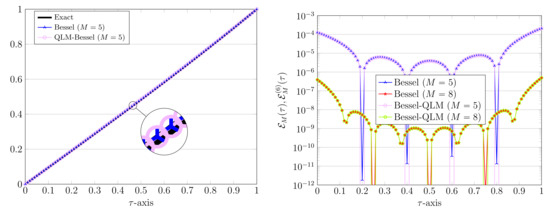
Figure 1. The graphs of exact and approximated solutions (left) and the related residual error functions (right) for $M=5,8$, and $r=5$ in Test case 1.

Our results with $M=8$ using both direct and linearization approaches are similar up to ten digits as follows

$$\begin{array}{cc}\hfill {\psi }_8^{(6)}(\tau ),{\psi }_8(\tau )& =8.2519\times {10}^{-6}{\tau }^8+1.8235\times {10}^{-5}{\tau }^7+1.9425\times {10}^{-5}{\tau }^6\hfill \\ \hfill & +9.4595\times {10}^{-4}{\tau }^5+5.3536\times {10}^{-6}{\tau }^4+0.03995880813{\tau }^3\hfill \\ \hfill & +1.9691\times {10}^{-7}{\tau }^2+0.9590437817\tau -6.276852\times {10}^{-17}.\hfill \end{array}$$

The residual errors achieved via the QLM-Bessel method for Test case 1 using $M=5,10,15$, and $M=20$ are graphically visualized in Figure 2. It can be seen that the approximate solutions are convergent exponentially when M is increased.

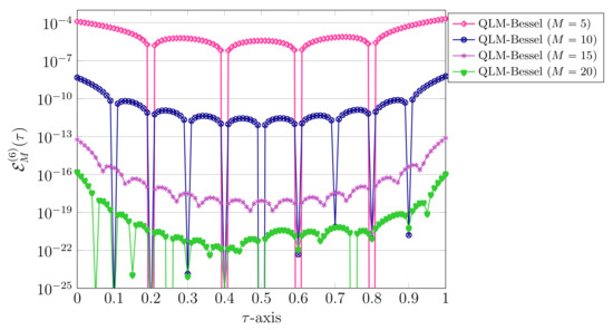
Figure 2. Comparison of residual error functions in QLM-Bessel for various $M=5,10,15,20$, and $r=5$ in Test case 1.

Finally, for this value of $\alpha$, we justify our results by comparing to other existing available numerical models. In this respect, we employ $M=9$ and report the numerical results in Table 1. We compare our computed solutions with the outcomes of the shifted Bessel Tau (SBT) method [20], the B-spline approach (BSA) [13], the double exponential sinc-Galerkin (DESG) method [15], and the modified non-linear shooting method (MNLSM) [9].

Table 1. Comparison of numerical solutions in Bessel/QLM-Bessel for Test case 1 using $M=9$ and various $\tau \in [0,1]$.

$\tau$	Bessel	QLM-Bessel	SBT [20]	BSA [13]	DESG [15]	MNLSM [9]
$0.1$	$0.0959443493$	$0.0959443493$	$0.095944350620621$	$0.095944$	$0.09594434932$	$0.09597247$
$0.2$	$0.1921287476$	$0.1921287477$	$0.192128750320282$	$0.192128$	$0.19212874768$	$0.19218506$
$0.3$	$0.2887944008$	$0.2887944009$	$0.288794404891654$	$0.288793$	$0.28879440094$	$0.28887905$
$0.4$	$0.3861848462$	$0.3861848464$	$0.386184851707410$	$0.386183$	$0.38618484638$	$0.38629807$
$0.5$	$0.4845471645$	$0.4845471648$	$0.484547171441282$	$0.484546$	$0.48454716477$	$0.48441684$
$0.6$	$0.5841332482$	$0.5841332485$	$0.584133256467667$	$0.584132$	$0.58413324848$	$0.58428140$
$0.7$	$0.6852011480$	$0.6852011483$	$0.685201157498259$	$0.685200$	$0.68520114831$	$0.68525684$
$0.8$	$0.7880165223$	$0.7880165227$	$0.788016532411673$	$0.788015$	$0.78801652269$	$0.78807945$
$0.9$	$0.8928542158$	$0.8928542162$	$0.892854224345211$	$0.892853$	$0.89285421616$	$0.89292601$

6.2. Test Case 2: $\alpha =1$

In this case, we first utilize $M=7$ in the Bessel-collocation method to obtain

$$\begin{array}{cc}\hfill {\psi }_7(\tau )& =0.0050297787{\tau }^7-0.0082098988{\tau }^6+0.020709825{\tau }^5-0.0049530270{\tau }^4\hfill \\ \hfill & +0.142486485{\tau }^3-0.0002918546382{\tau }^2+0.8452286916\tau .\hfill \end{array}$$

In fact, using $M=10$, the direct algorithm gives no reliable results. In the QLM-Bessel method, the corresponding approximate solution for $0\le \tau \le 1$ is

$$\begin{array}{cc}\hfill {\psi }_{10}^{(6)}(\tau )& =5.9125\times {10}^{-4}{\tau }^{10}-0.001726998{\tau }^9+0.0032385917{\tau }^8-0.001625926{\tau }^7\hfill \\ \hfill & +0.0020372912{\tau }^6+0.011214379{\tau }^5+2.4030\times {10}^{-4}{\tau }^4+0.140824035{\tau }^3\hfill \\ \hfill & +4.6403\times {10}^{-6}{\tau }^2+0.8452024383\tau -5.267094243\times {10}^{-109}.\hfill \end{array}$$

Figure 3 shows the residual error functions achieved via the QLM-Bessel method for Test case 2. In these experiments, we utilize $M=5,10,15$, and $M=20$. The validation includes a comparison with existing available numerical and experimental results, reported for the methods used in Table 1, and is listed in Table 2.

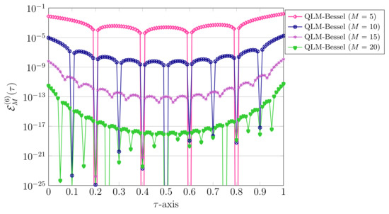
Figure 3. Comparison of residual error functions in QLM-Bessel for various $M=5,10,15,20$, and $r=5$ in Test case 2.

Table 2. Comparison of numerical solutions in QLM-Bessel for Test case 2 using $M=8,10$ and various $\tau \in [0,1]$.

$\tau$	$\mathit{M}=8$	$\mathit{M}=10$	LDM [11]	BSA [13]	DESG [15]	PSO [17]
$0.1$	$0.0846611308$	$0.0846612523$	$0.0846630897$	$0.084655$	$0.084661256642$	$0.0846685241$
$0.2$	$0.1701712882$	$0.1701713557$	$0.1701750442$	$0.170160$	$0.170171358273$	$0.1701736494$
$0.3$	$0.2573938770$	$0.2573939070$	$0.2573994845$	$0.257377$	$0.257393908175$	$0.2573894393$
$0.4$	$0.3472228668$	$0.3472228555$	$0.3472303763$	$0.347201$	$0.347222855224$	$0.3472184871$
$0.5$	$0.4405998884$	$0.4405998371$	$0.4406093753$	$0.440575$	$0.440599835276$	$0.4406021957$
$0.6$	$0.5385344936$	$0.5385344015$	$0.5385460046$	$0.538508$	$0.538534398177$	$0.5385424242$
$0.7$	$0.6421287494$	$0.6421286141$	$0.6421421393$	$0.642103$	$0.642128609348$	$0.6421341068$
$0.8$	$0.7526082754$	$0.7526081005$	$0.7526226886$	$0.752586$	$0.752608094135$	$0.7526041759$
$0.9$	$0.8713627684$	$0.8713625283$	$0.8713748860$	$0.871349$	$0.871362519949$	$0.8713530059$

Let us examine the impact of utilizing various values of parameter $\alpha$ on the obtained results. To this end, we fix $M=10$ and let $\alpha$ vary as $0.125,0.25,0.5,1,2,3,4$. The residual errors calculated via (38b) for $\tau \in [0,1]$ are presented in Figure 4. It can be concluded that the error function ${\mathcal{E}}_{10}^{(6)}(\tau )$ is a decreasing function with respect to $\alpha <1$, while it is inherently an increasing function with regard to $\alpha \ge 1$. In all cases, the maximum value of the errors occurred at $\tau =1$. Indeed, as investigated by Troesch [4], there exists a pole for the model problem (1), which is located at

$${\tau }_s=\frac{1}{\alpha }ln\left(\frac{8}{{\psi }^{\prime }(0)}\right).$$

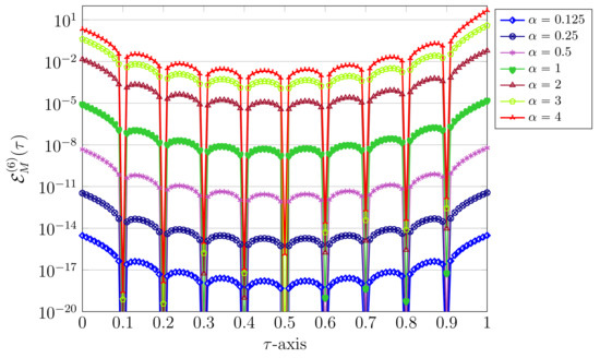
Figure 4. Comparison of residual error functions in QLM-Bessel for $M=10,r=5$, and various $\alpha$.

The values of ${\tau }_s$ approach to $\tau =1$ if one increases $\alpha >1$. The solution profiles at diverse $\alpha =0.125,0.25,0.5,1,2,3,4$, and $\alpha =5$ are presented in Figure 5. Finally, we validate our results by comparing our results with an optimal iterative scheme, which is based on the homotopy analysis method and the Green’s function technique (HAMG) [21]. In this respect, the residual errors ${\mathcal{E}}_M^{(6)}(\tau )$ using various $\alpha =1,1.5,2$, and $\alpha =2.5$ by the QLM-Bessel with $M=8,12,15$ computed at some points $\tau \in [0,1]$ are presented in Table 3. Looking at Table 3, one can infer that by increasing $\alpha$ the magnitude of errors achieved by our approach are getting smaller compared to the HAMG.

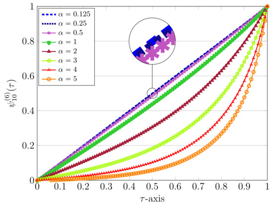
Figure 5. Numerical solutions in QLM-Bessel for $M=10,r=5$, and various $\alpha$.

Table 3. Comparison of numerical results in QLM-Bessel for $\alpha =1,1.5,2,2.5$, $M=8,12,15$, and some $\tau \in [0,1]$.

	$\alpha =1$		$\alpha =1.5$		$\alpha =2$		$\alpha =2.5$
$\mathbf{\tau }$	${\mathcal{E}}_{\mathbf{8}}^{(\mathbf{6})}(\mathbf{\tau })$	${\mathit{Res}}_{\mathbf{8}}$ [21]	${\mathcal{E}}_{\mathbf{8}}^{(\mathbf{6})}(\mathbf{\tau })$	${\mathit{Res}}_{\mathbf{8}}$	${\mathcal{E}}_{\mathbf{12}}^{(\mathbf{6})}(\mathbf{\tau })$	${\mathit{Res}}_{\mathbf{12}}$[21]	${\mathcal{E}}_{\mathbf{15}}^{(\mathbf{6})}(\mathbf{\tau })$	${\mathit{Res}}_{\mathbf{15}}$
$0.1$	$7.{56}_{-06}$	$2.{52}_{-9}$	$2.{59}_{-4}$	$8.{80}_{-6}$	v$3.{99}_{-05}$	$8.{68}_{-5}$	$5.{90}_{-05}$	$8.{39}_{-5}$
$0.2$	$2.{26}_{-06}$	$6.{36}_{-9}$	$7.{93}_{-5}$	$1.{79}_{-5}$	$6.{25}_{-06}$	$1.{98}_{-4}$	$2.{05}_{-18}$	$1.{84}_{-4}$
$0.3$	$8.{47}_{-07}$	$1.{23}_{-8}$	$3.{05}_{-5}$	$2.{69}_{-5}$	$1.{58}_{-06}$	$3.{49}_{-4}$	$6.{30}_{-07}$	$3.{09}_{-4}$
$0.4$	$3.{13}_{-07}$	$1.{99}_{-8}$	$1.{16}_{-5}$	$3.{38}_{-5}$	$4.{78}_{-07}$	$5.{30}_{-4}$	$7.{71}_{-16}$	$4.{52}_{-4}$
$0.5$	$9.{31}_{-65}$	$2.{66}_{-8}$	$0.{00}_{+0}$	$3.{50}_{-5}$	$1.{89}_{-35}$	$7.{00}_{-4}$	$2.{16}_{-07}$	$5.{87}_{-4}$
$0.6$	$3.{53}_{-07}$	$2.{65}_{-8}$	$1.{40}_{-5}$	$2.{45}_{-5}$	$6.{11}_{-07}$	$7.{96}_{-4}$	$5.{59}_{-14}$	$6.{75}_{-4}$
$0.7$	$1.{08}_{-06}$	$9.{43}_{-9}$	$4.{48}_{-5}$	$6.{35}_{-6}$	$2.{59}_{-06}$	$7.{63}_{-4}$	$1.{14}_{-06}$	$6.{96}_{-4}$
$0.8$	$3.{26}_{-06}$	$4.{30}_{-8}$	$1.{43}_{-4}$	$7.{46}_{-5}$	$1.{34}_{-05}$	$5.{91}_{-4}$	$4.{13}_{-13}$	$6.{67}_{-4}$
$0.9$	$1.{23}_{-05}$	$1.{73}_{-7}$	$5.{75}_{-4}$	$2.{35}_{-4}$	$1.{15}_{-04}$	$3.{17}_{-4}$	$2.{18}_{-04}$	$7.{46}_{-4}$

6.3. Test Case 3: $\alpha =5$

Let us consider the QLM-Bessel approach with $M=10$. Thus, the following approximation is achieved for $0\le \tau \le 1$

$$\begin{array}{cc}\hfill {\psi }_{10}^{(6)}(\tau )& =158.9257704{\tau }^{10}-698.6514572{\tau }^9+1338.269086{\tau }^8-1461.238116{\tau }^7\hfill \\ \hfill & +1000.941419{\tau }^6-445.5093877{\tau }^5+129.3704291{\tau }^4-23.60162081{\tau }^3\hfill \\ \hfill & +2.580220777{\tau }^2-0.08634442224\tau -2.180075438\times {10}^{-106}.\hfill \end{array}$$

Due to difficulties that arise in the Troesch’s model problem for large values of $\alpha$, the approximate solution ${\psi }_{10}^{(6)}(\tau )$ may be not so accurate as for the smaller values of $\alpha$. To this end, we need to take M sufficiently large to obtain the desired approximations. The impacts of diverse M on the numerical solutions as well as the residual errors are shown in Figure 6. We use $M=10,15$, and $M=20$ in the QLM-Bessel collocation method. Obviously, all approximated solutions are very close together while the corresponding residual errors are decreasing with respect to M.

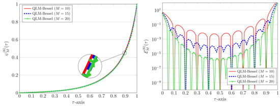
Figure 6. Comparison of numerical solutions in QLM-Bessel (left) and the related residual error functions (right) for $M=10,15,20$, and $r=5$ in Test case 3.

Next, we compare the results obtained via the QLM-Bessel approach for this test case. In this respect, we employ $M=15,25,$ and $M=35$. In Table 4, comparisons have been made with the results of the Fortran code called TWPBVP [13] as well as with the B-spline approach (BSA) [13], the double exponential sinc-Galerkin (DESG) method [15], and the shifted Jacobi–Gauss collocation method (SJGCM) [18]. The behavior of numerical solutions obtained by the QLM-Bessel taking various (large) values of parameter $\alpha =1,3,5,8,10,15,20,30,40,50,$ and $\alpha =100$ are depicted in Figure 7. Due to difficulties arising in the approximate solutions for the larger values of $\alpha$, we take $M=50$ to keep the accuracy at some acceptable level.

Table 4. Comparison of numerical solutions in QLM-Bessel for Test case 3 using $M=15,25,35$ and various $\tau \in [0,1]$.

$\tau$	$\mathit{M}=15$	$\mathit{M}=25$	$\mathit{M}=35$	TWPBVP [13]	BSM [13]	DSEG [15]	SJGCM [18]
$0.2$	$0.01124607$	$0.01083911$	$0.01076289$	$0.01075342$	$0.01002027$	$0.01075340$	$0.01078872$
$0.4$	$0.03372042$	$0.03328128$	$0.03322919$	$0.03320051$	$0.03099793$	$0.03320049$	$0.03338672$
$0.8$	$0.26145305$	$0.25868755$	$0.25845438$	$0.25821664$	$0.24170496$	$0.25821648$	$0.25956596$
$0.9$	$0.46159871$	$0.45601002$	$0.45554150$	$0.45506034$	$0.42461830$	$0.45506002$	$0.45706638$

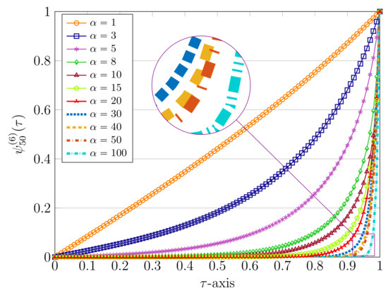
Figure 7. Numerical solutions in QLM-Bessel for $M=50,r=5$, and various $\alpha$.

7. Conclusions

An efficient collocation method based on the Bessel matrix representation combined with the quasi-linearization technique has been presented to find the solution of the two-point non-linear Troesch’s problem arising in the modeling of a plasma confinement problem and gas porous electrodes. In addition, a direct Bessel collocation method has been developed for the underlying model problem. The error analysis of Bessel functions was established theoretically and the related convergence verified experimentally through numerical simulations on diverse values of the sensitive parameter $\alpha$. Moreover, the comparisons of numerical solutions on different well-established schemes were performed to validate our presented approximation algorithms. It is found that the simulation results agree quite well in general with outcomes of existing schemes. The present QLM-Bessel method is broadly applicable and can be applied to solve diverse nonlinear model problems in engineering and science.

References

- Markin, V.S.; Chernenko, A.A.; Chizmadehev, Y.A.; Chirkov, Y.G. Aspects of the theory of gas porous electrodes. In Fuel Cells: Their Electrochemical Kinetics; Bagotskii, V.S., Vasilev, Y.B., Eds.; Consultants Bureau: New York, NY, USA, 1966; pp. 21–33. [Google Scholar]
- Gidaspow, D.; Baker, B.S. A model for discharge of storage batteries. J. Electrochem. Soc. 1973, 120, 1005–1010. [Google Scholar] [CrossRef]
- Weibel, E.S. On the confinement of a plasma by magnetostatic fields. Phys. Fluids 1959, 2, 52–56. [Google Scholar] [CrossRef]
- Troesch, B.A. Intrinsic Difficulties in the Numerical Solution of a Boundary Value Problem; Internal Report NN-142; TRW, Inc.: Redondo Beach, CA, USA, 1960. [Google Scholar]
- Troesch, B.A. A simple approach to a sensitive two-point boundary value problem. J. Comput. Phys. 1976, 21, 279–290. [Google Scholar] [CrossRef]
- Roberts, S.; Shipman, J. On the closed form solution of Troesch’s problem. J. Comput. Phys. 1976, 21, 291–304. [Google Scholar] [CrossRef]
- Jones, D.J. Solution of Troesch’s and other two point boundary value problems by shooting techniques. J. Comput. Phys. 1973, 12, 42–434. [Google Scholar] [CrossRef]
- Chang, S. Numerical solution of Troesch’s problem by simple shooting method. Appl. Math. Comput. 2010, 216, 3303–3306. [Google Scholar] [CrossRef]
- Alias, N.; Manaf, A.; Ali, A.; Habib, M. Solving Troesch’s problem by using modified nonlinear shooting method. J. Teknolog. 2016, 78, 45–52. [Google Scholar] [CrossRef] [Green Version]
- Scott, M. On the conversion of boundary-value problems into stable initial-value problems via several invariant imbedding algorithms. In Numerical Solutions of Boundary-Value Problems for Ordinary Differential Equations; Aziz, A.K., Ed.; Academic Press: New York, NY, USA, 1975; pp. 89–149. [Google Scholar]
- Khuri, S.A. A numerical algorithm for solving the Troesch’s problem. Int. J. Comput. Math. 2003, 80, 493–498. [Google Scholar] [CrossRef]
- Feng, X.; Mei, L.; He, G. An efficient algorithm for solving Troesch’s problem. Appl. Math. Comput. 2007, 189, 500–507. [Google Scholar] [CrossRef]
- Khuri, S.A.; Sayfy, A. Troesch’s problem: A B-Spline collocation approach. Math. Comput. Model. 2011, 54, 1907–1918. [Google Scholar] [CrossRef]
- Zarebnia, M.; Sajjadian, M. The sinc-Galerkin method for solving Troesch’s problem. Math. Comput. Model. 2012, 56, 218–228. [Google Scholar] [CrossRef]
- Nabati, M.; Jalalvand, M. Solution of Troesch’s problem through double exponential Sinc-Galerkin method. Comput. Methods Differ. Equ. 2017, 5, 141–157. [Google Scholar]
- Temimi, H. A discontinuous Galerkin finite element method for solving the Troesch’s problem. Appl. Math. Comput. 2012, 219, 521–529. [Google Scholar] [CrossRef]
- Raja, M.A.Z. Stochastic numerical treatment for solving Troesch’s problem. Infor. Sci. 2014, 279, 860–873. [Google Scholar] [CrossRef]
- Doha, E.H.; Baleanu, D.; Bahrawi, A.H.; Hafez, R.M. A Jacobi collocation method for Troesch’s problem in plasma physics. Proc. Rom. Acad. A 2014, 15, 130–138. [Google Scholar]
- Temimi, H.; Ben-Romdhane, M.; Ansari, A.R.; Shishkin, G.I. Finite difference numerical solution of Troesch’s problem on a piecewise uniform Shishkin mesh. Calcolo 2017, 54, 225–242. [Google Scholar] [CrossRef]
- Parand, K.; Ghaderi, A.; Delkhosh, M.; Pourgholi, R. A matrix formulation of the Tau method for the numerical solution of non-linear problems. arXiv 2017, arXiv:1708.06941. [Google Scholar]
- Singh, R. An iterative technique for solving a class of local and nonlocal elliptic boundary value problems. J. Math. Chem. 2020, 58, 1874–1894. [Google Scholar] [CrossRef]
- Rufai, M.A.; Ramos, H. One-step hybrid block method containing third derivatives and improving strategies for solving Bratu’s and Troesch’s problems. Numer. Math. Theor. Meth. Appl. 2020, 13, 946–972. [Google Scholar]
- Sahlan, M.N.; Afshari, H. Three new approaches for solving a class of strongly nonlinear two-point boundary value problems. Bound. Value Probl. 2021, 1, 1–21. [Google Scholar]
- Krall, H.L.; Frink, O. A new class of orthogonal polynomials: The Bessel polynomials. Trans. Am. Math. Soc. 1949, 65, 100–115. [Google Scholar] [CrossRef]
- Izadi, M.; Cattani, C. Generalized Bessel polynomial for multi-order fractional differential equations. Symmetry 2020, 12, 1260. [Google Scholar] [CrossRef]
- Izadi, M.; Srivastava, H.M. An efficient approximation technique applied to a non-linear Lane-Emden pantograph delay differential model. Appl. Math. Comput. 2021, 401, 1–10. [Google Scholar]
- Izadi, M. Numerical approximation of Hunter-Saxton equation by an efficient accurate approach on long time domains. UPB Sci. Bull. Ser. A 2021, 83, 291–300. [Google Scholar]
- Izadi, M.; Cattani, C. Solution of nonlocal fractional-order boundary value problems by an effective accurate approximation method. Appl. Ana. Optim. 2021, 5, 29–44. [Google Scholar]
- Yüzbaşi, Ş. Numerical solutions of singularly perturbed one-dimensional parabolic convection-diffusion problems by the Bessel collocation method. Appl. Math. Comput. 2013, 220, 305–315. [Google Scholar] [CrossRef]
- Yüzbaşi, Ş. A collocation method based on the Bessel functions of the first kind for singular perturbated differential equations and residual correction. Math. Meth. Appl. Sci. 2015, 38, 3033–3042. [Google Scholar] [CrossRef]
- Izadi, M.; Srivastava, H.M. Numerical approximations to the nonlinear fractional-order Logistic population model with fractional-order Bessel and Legendre bases. Chaos Solitons Fract. 2021, 145, 1–11. [Google Scholar] [CrossRef]
- Yüzbaşi, Ş. A collocation approach for solving two-dimensional second-order linear hyperbolic equations. Appl. Math. Comput. 2018, 338, 101–114. [Google Scholar] [CrossRef]
- Izadi, M. A comparative study of two Legendre-collocation schemes applied to fractional logistic equation. Int. J. Appl. Comput. Math. 2020, 6, 71. [Google Scholar] [CrossRef]
- Srivastava, H.M.; Saad, K.M. A comparative study of the fractional-order clock chemical model. Mathematics 2020, 8, 1436. [Google Scholar] [CrossRef]
- Izadi, M.; Afshar, M. Solving the Basset equation via Chebyshev collocation and LDG methods. J. Math. Model. 2021, 9, 61–79. [Google Scholar]
- Singh, H.; Srivastava, H.M. Numerical simulation for fractional-order Bloch equation arising in nuclear magnetic resonance by using the Jacobi polynomials. Appl. Sci. 2020, 10, 2850. [Google Scholar] [CrossRef] [Green Version]
- Hashemizadeh, E.; Ebadi, M.A.; Noeiaghdam, S. Matrix method by Genocchi polynomials for solving nonlinear Volterra integral equations with weakly singular kernels. Symmetry 2020, 12, 2105. [Google Scholar] [CrossRef]
- Yüzbaşi, Ş.; Savasaneril, N.B. Hermite polynomial approach for solving singular perturb delay differential equation. J. Sci. Arts 2020, 20, 845–854. [Google Scholar] [CrossRef]
- Bellman, R.E.; Kalaba, R.E. Quasilinearization and Nonlinear Boundary-Value Problems; Elsevier Publishing Company: New York, NY, USA, 1965. [Google Scholar]
- Mandelzweig, V.B.; Tabakin, F. Quasilinearization approach to nonlinear problems in physics with application to nonlinear ODEs. Comput. Phys. Commun. 2001, 141, 268–281. [Google Scholar] [CrossRef] [Green Version]
- Izadi, M. An approximation technique for first Painlevé equation. TWMS J. App. Eng. Math. 2021, 11, 739–750. [Google Scholar]
Publisher’s Note: MDPI stays neutral with regard to jurisdictional claims in published maps and institutional affiliations. |
© 2021 by the authors. Licensee MDPI, Basel, Switzerland. This article is an open access article distributed under the terms and conditions of the Creative Commons Attribution (CC BY) license (https://creativecommons.org/licenses/by/4.0/).