Eigenvalue Estimates via Pseudospectra ^†

Abstract

In this note, given a matrix $A\in {\mathbb{C}}^{n\times n}$ (or a general matrix polynomial $P\left(z\right)$, $z\in \mathbb{C}$) and an arbitrary scalar ${\lambda }_0\in \mathbb{C}$, we show how to define a sequence ${\left\{{\mu }_k\right\}}_{k\in \mathbb{N}}$ which converges to some element of its spectrum. The scalar ${\lambda }_0$ serves as initial term (${\mu }_0={\lambda }_0$), while additional terms are constructed through a recursive procedure, exploiting the fact that each term ${\mu }_k$ of this sequence is in fact a point lying on the boundary curve of some pseudospectral set of A (or $P\left(z\right)$). Then, the next term in the sequence is detected in the direction which is normal to this curve at the point ${\mu }_k$. Repeating the construction for additional initial points, it is possible to approximate peripheral eigenvalues, localize the spectrum and even obtain spectral enclosures. Hence, as a by-product of our method, a computationally cheap procedure for approximate pseudospectra computations emerges. An advantage of the proposed approach is that it does not make any assumptions on the location of the spectrum. The fact that all computations are performed on some dynamically chosen locations on the complex plane which converge to the eigenvalues, rather than on a large number of predefined points on a rigid grid, can be used to accelerate conventional grid algorithms. Parallel implementation of the method or use in conjunction with randomization techniques can lead to further computational savings when applied to large-scale matrices.

1. Introduction

The theory of pseudospectra originates in numerical analysis and can be traced back to Landau [1], Varah [2], Wilkinson [3], Demmel [4], and Trefethen [5], motivated by the need to obtain insights into systems evolving in ways that the eigenvalues alone could not explain. This is especially true in problems where the underlying matrices or linear operators are non-normal or exhibit in some sense large deviations from normality. A better understanding of such systems can be gained through the concept of pseudospectrum, which, for a matrix $A\in {\mathbb{C}}^{n\times n}$ and a positive parameter $ϵ>0$, was introduced as the subset of the complex plane that is bounded by the ${ϵ}^{-1}$–level set of the norm of the resolvent $∥{(\mu I-A)}^{-1}∥$. A second definition stated in terms of perturbations characterizes the elements of this set as eigenvalues of some perturbation $A+E$ with $∥E∥\le ϵ$. In this sense, the notion of pseudospectrum provides information that goes beyond eigenvalues, while retaining the advantage of being a natural extension of the spectral set. In fact, for different values of magnitude $ϵ$, pseudospectrum provides a global perspective on the effects of perturbations; this is in stark contrast to the concept of condition number, where only the worst-case scenario is considered.

On one hand, pseudospectrum may be used as a visualization tool to reveal information regarding the matrix itself and the sensitivity of its eigenvalues. Applications within numerical analysis include convergence of nonsymmetric matrix iterations [6], backward error analysis of eigenvalue algorithms [7], and stability of spectral methods [8]. On the other hand, it is a versatile tool that has been used to obtain quantitative bounds on the transient behavior of differential equations in finite time, which may deviate from the long-term asymptotic behavior [9]. Important results involving pseudospetra have been also been obtained in the context of spectral theory and spectral properties of banded Toeplitz matrices [10,11]. Although emphasis has been placed on the standard eigenproblem, attention has also been drawn to matrix pencils [12] and more general matrix polynomials [13,14] arising in vibrating systems, control theory, etc. For a comprehensive overview of this research field and its applications, the interested reader may refer to [15].

In this note, we propose an application of pseudospectral sets as a mean to obtain eigenvalue estimates in the vicinity of some complex scalar. In particular, given a matrix (or a general matrix polynomial) and a scalar ${\lambda }_0\in \mathbb{C}$, we construct a sequence ${\left\{{\mu }_k\right\}}_{k\in \mathbb{N}}$ that converges to some element of its spectrum. The scalar ${\lambda }_0$ serves as initial term (${\mu }_0={\lambda }_0$), while additional terms are constructed through an iterative procedure, exploiting the fact that each term ${\mu }_k$ of this sequence is in fact a point lying on the boundary curve of some pseudospectral set. Then, the next term in the sequence is detected in the perpendicular direction to the tangent line at the point ${\mu }_k$. Repeating the construction for a tuple of initial points encircling the spectrum, several peripheral eigenvalues are approximated. Since the pseudospectrum may be disconnected, this procedure allows the identification of individual connected components and, as a by-product, a convenient and numerically efficient procedure for approximate pseudospectrum computation emerges. Moreover, this approach is clearly amenable to parallelization or randomization and can lead to significant computational savings when applied to probems involving large–scale matrices.

Our paper is organized as follows. In Section 2, we provide the necessary theoretical background on the method and provide examples for the constant matrix case. As confirmed by numerical experiments, the method can provide a sufficiently accurate pseudospectrum computation at a much-reduced computational cost, especially in cases where the spectrum is convexly independent (i.e., each eigenvalue does not lie in the convex hull of the others) or exhibits large eigenvalue gaps. A second application of the method on Perron-root approximation for non–negative matrices is presented. Then, Section 3 shows how the procedure may be modified to estimate the spectrum of more general matrix polynomials. Numerical experiments showcasing the application of the method on damped mass–spring and gyroscopic systems conclude the paper.

2. Eigenvalues via Pseudospectra

Let the matrix $A\in {\mathbb{C}}^{n\times n}$ with spectrum $\sigma \left(A\right)=\left\{\mu \in \mathbb{C}:det(\mu I-A)=0\right\}$, where $det(·)$ denotes the determinant of a matrix. With respect to the ${∥·∥}_2$–norm, the pseudospectrum of A is defined by

$$\begin{array}{cc}\hfill {\sigma }_{ϵ}\left(A\right)& =\left\{\mu \in \mathbb{C}:\frac{1}{{∥{(\mu I-A)}^{-1}∥}_2}\le ϵ\right\}\hfill \\ \hfill & =\left\{\mu \in \mathbb{C}:\mu \in \sigma (A+E)\mathrm{for}\mathrm{some}E\in {\mathbb{C}}^{n\times n}\mathrm{with}∥E∥\le ϵ\right\}\hfill \\ \hfill & =\left\{\mu \in \mathbb{C}:s_{min}(\mu I-A)\le ϵ\right\},\hfill \end{array}$$

where $s_{min}(·)$ denotes the smallest singular value of a matrix and $ϵ>0$ is the maximum norm of admissible perturbations.

For every choice of increasing positive parameters $0<{ϵ}_1<{ϵ}_2<{ϵ}_3<\dots$, the corresponding closed, strictly nested sequence of pseudospectra

$${\sigma }_{{ϵ}_1}\left(A\right)\subset {\sigma }_{{ϵ}_2}\left(A\right)\subset {\sigma }_{{ϵ}_3}\left(A\right)\subset \dots$$

is obtained. In fact, the respective boundaries satisfy the inclusions

$$\begin{array}{cc}\hfill \partial {\sigma }_{{ϵ}_1}\left(A\right)& \subseteq \left\{\mu \in \mathbb{C}:s_{min}(\mu I-A)={ϵ}_1\right\}\hfill \\ \hfill \partial {\sigma }_{{ϵ}_2}\left(A\right)& \subseteq \left\{\mu \in \mathbb{C}:s_{min}(\mu I-A)={ϵ}_2\right\}\hfill \\ \hfill \partial {\sigma }_{{ϵ}_3}\left(A\right)& \subseteq \left\{\mu \in \mathbb{C}:s_{min}(\mu I-A)={ϵ}_3\right\}\hfill \\ \hfill ⋮& ⋮\hfill \end{array}$$

It is also clear that, for any $\lambda \in \sigma \left(A\right)$, $s_{min}(\lambda I-A)=0$.

Our objective now is to exploit the properties of these sets to detect an eigenvalue of A in the vicinity of a given scalar ${\lambda }_0\in \mathbb{C}\backslash \sigma \left(A\right)$. This given point of interest may be considered to lie on the boundary of some pseudospectral set, i.e., there exists some non–negative parameter ${\widehat{ϵ}}_1>0$, such that

$$\begin{array}{cc}\hfill {\lambda }_0\in \partial {\sigma }_{{\widehat{ϵ}}_1}\left(A\right)& \subseteq \left\{\mu \in \mathbb{C}:s_{min}(\mu I-A)={\widehat{ϵ}}_1\right\}.\hfill \end{array}$$

(1)

Indeed, points satisfying the equality $s_{min}(\mu I-A)=ϵ$ for some $ϵ>0$ and lying in the interior of ${\sigma }_{ϵ}\left(A\right)$ are finite in number. Thus, in the generic case, we may think of the inclusion (1) as an equality.

We consider the real–valued function $g_A:\mathbb{C}\to {\mathbb{R}}_{+}$ with $g_A\left(z\right)=s_{min}(zI-A)$. In the process of formulating a curve-tracing algorithm for pseudospectrum computation [16], Brühl analyzed $g_A\left(z\right)$ and, identifying $\mathbb{C}\equiv {\mathbb{R}}^2$, noted that its differentiability is explained by the following Theorem in [17]:

Theorem 1.

Let the matrix valued function $P\left(\chi \right):{\mathbb{R}}^d\to {\mathbb{C}}^{n\times n}$ be real analytic in a neighborhood of ${\chi }_0=\left(x_0^1,\dots ,x_0^d\right)$ and let ${\sigma }_0$ a simple nonzero singular value of $P\left({\chi }_0\right)$ with $u_0$, $v_0$ its associated left and right singular vectors, respectively.

Then, there exists a neighborhood $\mathcal{N}$ of ${\chi }_0$ on which a simple nonzero singular value $\sigma \left(\chi \right)$ of $P\left(\chi \right)$ is defined with corresponding left and right singular vectors $u\left(\chi \right)$ and $v\left(\chi \right)$, respectively, such that $\sigma \left({\chi }_0\right)={\sigma }_0$, $u\left({\chi }_0\right)=u_0$, $v\left({\chi }_0\right)=v_0$ and the functions σ, u, v are real analytic on $\mathcal{N}$. The partial derivatives of $\sigma \left(\chi \right)$ are given by

$$\frac{\partial s\left({\chi }_0\right)}{\partial {\chi }^j}=\mathrm{Re}\left(u_0^{*}\frac{\partial P\left({\chi }_0\right)}{\partial {\chi }^j}{v}_0\right),j=1,\dots ,d.$$

Hence, recalling (1) and assuming ${\widehat{ϵ}}_1$ is a simple singular value of the matrix $P\left({\lambda }_0\right)={\lambda }_{0}I-A$, then

$$\nabla s_{min}(zI-A){|}_{z={\lambda }_0}=\left(\mathrm{Re}\left(v_{min}^{*}{u}_{min}\right),\mathrm{Im}\left(v_{min}^{*}{u}_{min}\right)\right)=v_{min}^{*}{u}_{min},$$

where $u_{min}$ and $v_{min}$ denote the left and right singular vectors of ${\lambda }_{0}I-A$ associated to ${\widehat{ϵ}}_1=s_{min}({\lambda }_{0}I-A)$, respectively [16] (Corollary 2.2).

On the other hand, if $\lambda$ is an eigenvalue of A near ${\lambda }_0$, it holds $\left|\lambda -{\lambda }_0\right|\le {\widehat{ϵ}}_1$. The latter observation follows from the fact that

$$\begin{array}{cc}\hfill {\sigma }_{ϵ}\left(A\right)& \supseteq \sigma \left(A\right)+D(0,ϵ)\hfill \\ \hfill & =\left\{z\in \mathbb{C}:\mathrm{dist}(z,\sigma (A\left)\right)\le ϵ\right\},\hfill \end{array}$$

where $D(0,ϵ)=\left\{z\in \mathbb{C}:\left|z\right|\le ϵ\right\}$ and equality holds for normal matrices. So, the scalar

$$\begin{array}{cc}\hfill {\mu }_1& ={\lambda }_0-{\widehat{ϵ}}_1·\frac{\nabla s_{min}(zI-A)}{\left|\nabla s_{min}(zI-A)\right|}{|}_{z={\lambda }_0}\hfill \\ \hfill & ={\lambda }_0-s_{min}({\lambda }_{0}I-A)·\frac{v_{min}{\left({\lambda }_0\right)}^{*}{u}_{min}\left({\lambda }_0\right)}{\left|v_{min}{\left({\lambda }_0\right)}^{*}{u}_{min}\left({\lambda }_0\right)\right|}\hfill \end{array}$$

can be considered to be an estimate of eigenvalue $\lambda$. In particular, ${\lambda }_0\in \partial {\sigma }_{{\widehat{ϵ}}_1}\left(A\right)$ and ${\mu }_1$ lies in the interior of ${\sigma }_{{\widehat{ϵ}}_1}\left(A\right)$. Moreover, the sequence

$$\begin{array}{cc}\hfill {\mu }_0& ={\lambda }_0\hfill \\ \hfill {\mu }_1& ={\mu }_0-s_{min}({\mu }_{0}I-A)·\frac{v_{min}{\left({\mu }_0\right)}^{*}{u}_{min}\left({\mu }_0\right)}{\left|v_{min}{\left({\mu }_0\right)}^{*}{u}_{min}\left({\mu }_0\right)\right|}\hfill \\ \hfill {\mu }_2& ={\mu }_1-s_{min}({\mu }_{1}I-A)·\frac{v_{min}{\left({\mu }_1\right)}^{*}{u}_{min}\left({\mu }_1\right)}{\left|v_{min}{\left({\mu }_1\right)}^{*}{u}_{min}\left({\mu }_1\right)\right|}\hfill \\ \hfill ⋮& ⋮\hfill \\ \hfill {\mu }_k& ={\mu }_{k-1}-s_{min}({\mu }_{k-1}I-A)·\frac{v_{min}{\left({\mu }_{k-1}\right)}^{*}{u}_{min}\left({\mu }_{k-1}\right)}{\left|v_{min}{\left({\mu }_{k-1}\right)}^{*}{u}_{min}\left({\mu }_{k-1}\right)\right|}\hfill \end{array}$$

(2)

converges to $\lambda$.

The above process requires the computation of the triplet

$$\left(s_{min}({\mu }_{k}I-A),u_{min}\left({\mu }_k\right),v_{min}\left({\mu }_k\right)\right)$$

at every point ${\mu }_k$; see [18].

Remark. To avoid the computational burden of computing the (left and right) singular vectors, a cheaper alternative would be to consider at each iteration ($k=0,1,2,\dots$) the canonical octagon with vertices

$$p_{k,j}={\mu }_k+e^{\mathbf{i}\left(j\frac{\pi }{4}\right)}·s_{min}\left({\mu }_{k}I-A\right),j=0,1,2,\dots 7$$

instead and simply compute

$${\theta }_{k,j}=s_{min}\left(p_{k,j}I-A\right),j=0,1,2,\dots 7.$$

In this case, instead of (2), we can set

$${\mu }_{k+1}={\mu }_k+e^{\mathbf{i}\left(j_0\frac{\pi }{4}\right)}·{\theta }_{k,j_0}$$

with $j_0$ such that

$${\theta }_{k,j_0}=\underset{j=0,1,2,\dots ,7}{min}{\theta }_{k,j}=\underset{j=0,1,2,\dots ,7}{min}\left(s_{min}\left(p_{k,j}I-A\right)\right).$$

2.1. Numerical Experiments

2.1.1. Pseudospectrum Computation

The approximating sequences in (2) may be utilized to implement a computationally cheap procedure to visualize matrix pseudospectra, at least in cases where the order of the matrix is small or when its spectrum exhibits large eigenvalue gaps. Several related techniques for pseudospectrum computation have appeared in the literature. These fall largely into two categories: grid [14] and path-following algorithms [16,19,20,21]. Grid algorithms begin by evaluating the function $s_{min}(zI-A)$ on a predefined grid on the complex plane and lead to a graphical visualization of the boundary $\partial {\sigma }_{ϵ}\left(A\right)$ by plotting the $ϵ$-contours of $s_{min}(zI-A)$. This approach faces two severe challenges; namely, the requirement of a–priori information on the location of the spectrum to correctly identify a suitable region to discretize, as well as the typically large number of grid points the computations have to be performed upon. path-following algorithms, on the other hand, require an initial step to detect a starting point on the curve $\partial {\sigma }_{ϵ}\left(A\right)$ and then proceed to compute additional boundary points for each connected component of ${\sigma }_{ϵ}\left(A\right)$. The main drawbacks of this latter approach lie in the difficulty in performing the initial step and the need to correctly identify every connected component of ${\sigma }_{ϵ}\left(A\right)$ in order to repeat the procedure and properly trace its boundary. Moreover, cases where pseudospectrum computation is required for a whole tuple of parameters $ϵ$ drastically compromise the efficiency of path-following algorithms.

Our approach is to use the approximating sequences (2) to decrease the number of singular value evaluations and therefore speed up the computation of pseudospectra. The basic steps are outlined as follows:

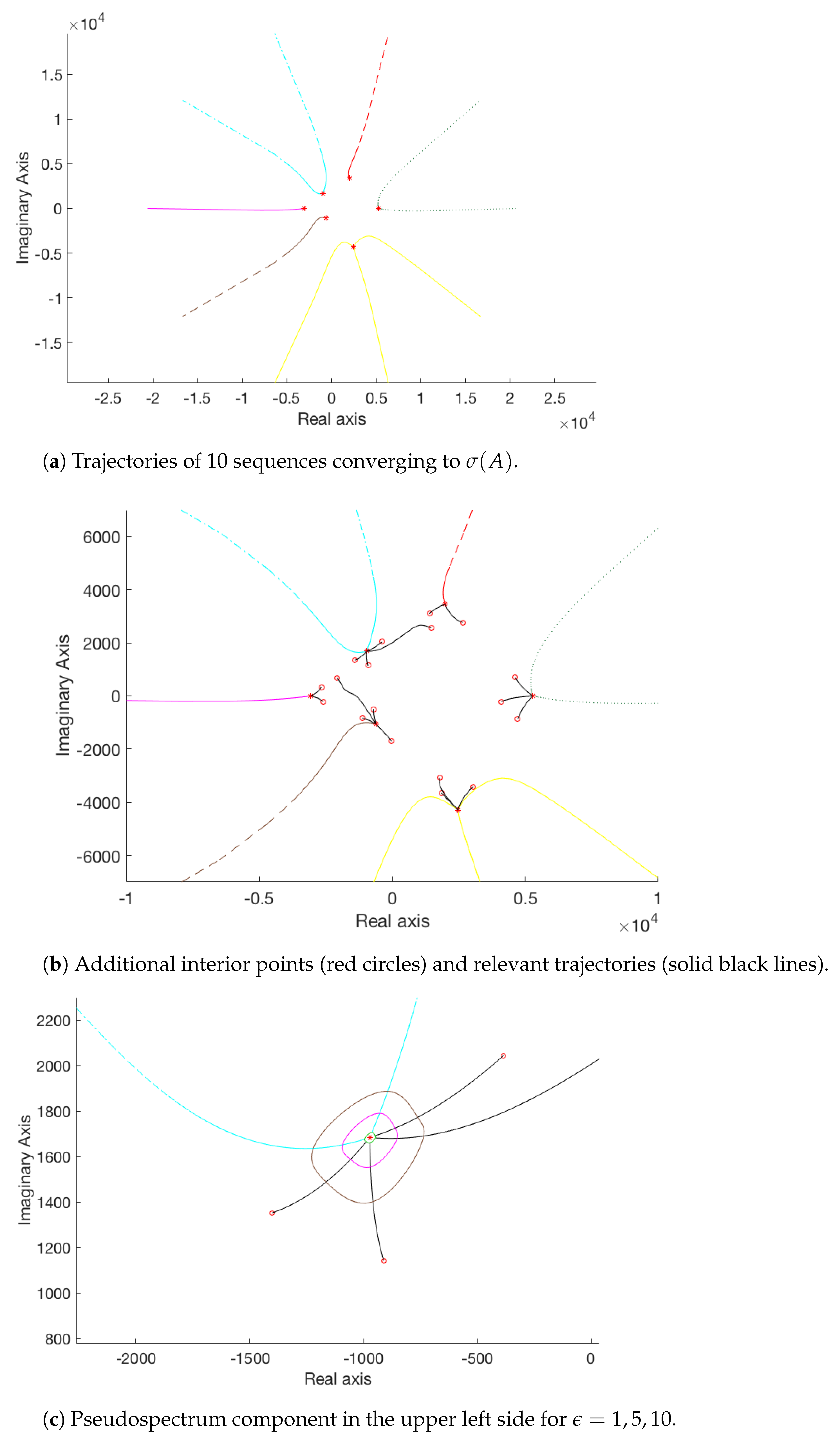
• Select a tuple of initial points ${\left\{{\mu }_0^j\right\}}_{j=1}^s\in \mathbb{C}$ encircling the spectrum; for instance, these can be chosen on the circle $\left\{z\in \mathbb{C}:\left|z\right|=∥A∥\right\}$.
• Construct eigenvalue approximating sequences ${\left\{{\mu }_k^j\right\}}_{k=0}^{n_j}$ ($j=1,\dots ,s$), as in (2). If ${ϵ}_k^j>0$ ($k=1,\dots ,n_j$) are such that ${\mu }_k^j\in \partial {\sigma }_{{ϵ}_k^j}\left(A\right)$, the length $n_j$ of each sequence is determined, so that $s_{min}({\mu }_{n_j}^{j}I-A)\le {ϵ}_0$ for all $j=1,\dots ,s$, where ${ϵ}_0$ is some prefixed parameter value. In other words, ${ϵ}_0$ indicates the tolerance with which the approached by the constructed sequences eigenvalues should be approximated and corresponds to the minimum parameter for which pseudospectra will be computed.
• Classify the sequences into distinct clusters, according to the proximity of their final terms. This step may be performed using a k-means clustering algorithm, using a suitable criterion to evaluate the optimal number of groups.
• Compute

  $$u=\underset{j=1,\dots ,s}{min}\underset{j=1,\dots ,n_j}{max}{ϵ}_k^j(>{ϵ}_0)\mathrm{and}\ell =\underset{j=1,\dots ,s}{max}\underset{j=1,\dots ,n_j}{min}{ϵ}_k^j(<{ϵ}_0).$$
• If necessary, repeat the procedure for t additional points between the centroids of the detected clusters, constructing additional sequences, so that

  $$\underset{j=s+1,\dots ,s+t}{min}\underset{j=1,\dots ,n_j}{max}{ϵ}_k^j>u\mathrm{and}\underset{j=s+1,\dots ,s+t}{max}\underset{j=1,\dots ,n_j}{min}{ϵ}_k^j<\ell .$$
• Detect boundary points of ${\sigma }_{ϵ}\left(A\right)$ for any choice of parameters $ϵ\in [\ell ,u]$ along the polygonal chains formed by the total of $s+t$ constructed sequences of points by interpolation.
• Fit closed spline curves passing through the respective sets of boundary points in $\partial {\sigma }_{ϵ}\left(A\right)$ for the various choices of $ϵ\in [\ell ,u]$ to obtain sketches of the corresponding pseudospectra ${\sigma }_{ϵ}\left(A\right)$.

The proposed method successfully localizes the spectrum, initiating the procedure with a restricted number of points. Then, singular value computations are kept to a minimum by considering points only on the constructed sequences. Pseudospectrum components corresponding to peripheral eigenvalues $\lambda \notin \mathrm{co}\left(\sigma \left(A\right)\backslash \left\{\lambda \right\}\right)$ not in the convex hull of the other eigenvalues, are thus extremely easy to identify. This approach is also well–suited to cases, where the matrix has convexly independent spectrum; i.e., when $\lambda \notin \mathrm{co}\left(\sigma \left(A\right)\backslash \left\{\lambda \right\}\right)$, for every $\lambda \in \sigma \left(A\right)$. Moreover, it is clearly amenable to parallelization, which could lead to significant computational savings in cases of large matrices.

Application 1.

We consider a random matrix $A\in {\mathbb{C}}^{6\times 6}$, the sole constraint being that its eigenvalues are distant form each other; the real and imaginary parts of its entries follow the standardized normal distribution scaled by ${10}^4$. For the proposed procedure, we select initial points ${\left\{{\mu }_0^j\right\}}_{j=1}^{10}\subset \left\{z\in \mathbb{C}:\left|z\right|={∥A∥}_1\right\}$ and exploit the fact that the corresponding sequences ${\left\{{\mu }_k^j\right\}}_{k=0}^{n_j}$ generated as in (2) converge to some element of $\sigma \left(A\right)$. The number $n_j$ of terms in each sequence $(j=1,\dots 10)$ is determined, so that all values ${\left\{s_{min}({\mu }_{n_j}^{j}I-A)\right\}}_{j=1}^{10}$ do not exceed ${ϵ}_0=0.5$. The sequences are organized into distinct clusters, grouping together those sequences which approximate the same element of $\sigma \left(A\right)$. This grouping is performed using a k-means clustering algorithm, where the optimal number of clusters is evaluated via the silhouette criterion and using a distance metric based on the sum of absolute differences between points. Since six different groups are identified, clearly all elements of $\sigma \left(A\right)$ have been sufficiently approximated by at least one of the sequences. For an illustration, refer to Figure 1a; different colors have been used to differentiate between polygonal chains corresponding to distinct clusters. The construction so far required 914 singular value computations. Having calculated all parameter values ${ϵ}_k^j$ such that ${\mu }_k^j\in \partial {\sigma }_{{ϵ}_k^j}\left(A\right)$ during the previous procedure, it is possible to interpolate between these known points along the trajectories formed by ${\left\{{\mu }_k^j\right\}}_{k=0}^{n_j}$ ($j=1,\dots 10$) to approximate boundary points of $\partial {\sigma }_{ϵ}\left(A\right)$ for selected values $ϵ>{ϵ}_0=0.5$. Since all ten trajectories converge to eigenvalues from points encircling $\sigma \left(A\right)$, to obtain better pseudospectra approximations, it is necessary to repeat the procedure for additional suitably selected points. Hence, for each cluster we consider three additional points; see Figure 1b. In particular, denoting $c_1,\dots c_6$ the centroids of the clusters, for each j we consider the three centroids ${\left\{c_{j,k}\right\}}_{k=1}^3$ which lie closest to $c_j$ and take the convex combinations

$$p_k^j=\frac{1}{6}\left(5c_j+c_{j,k}\right),k=1,2,3.$$

Then, additional sequences corresponding to these extra points are constructed so that the desired parameter values of ϵ for which pseudospectra should be computed (in this instance, the triple of $ϵ=1,5,10\in [\ell ,u]$) may be interpolated within these trajectories, as for the ten initial ones. This imposes an extra cost of 1170 additional singular value computations (2084 in total). The resulting approximations of the pseudospectra components identified by the upper left corner trajectories for $ϵ=1,5,10$ are depicted in greater detail in Figure 1c; the relevant eigenvalue is indicated by “*”.

Figure 1. Pseudospectrum computation for random $A\in {\mathbb{C}}^{6\times 6}$ with spectral gaps, using 10 initial points.

An advantage of this procedure is that it does not require some a–priori knowledge of the initial region $\Omega$ on the complex plane where the spectrum is located. In fact, the very nature of this specific example, whose spectrum covers a wide area $\Omega$, would render computations on a suitable grid impractical. Another way in which this method diverges from conventional grid algorithms is in that the computations are performed on a dynamically chosen set of points, iteratively selected as the corresponding trajectories converge to peripheral eigenvalues and identify the relevant pseudospectrum components, rather than on a large number of predefined points on a rigid grid.

Application 2.

To demonstrate how the procedure works in cases of larger matrices, in this application we examine the matrix $A={10}^{-7}·Pores2$, where $Pores2$ is a $1024\times 1024$ matrix from the Harwell-Boeing sparse matrix collection [22] related to a non–symmetric computational fluid dynamics problem. Here, the factor ${10}^{-7}$ is used for scaling purposes and is related to the norm–${∥·∥}_1$ order of the matrix under consideration. Initiating the procedure with 30 equidistributed points on the circle $\left\{z\in \mathbb{C}:\left|z\right|=\frac{1}{2}{∥A∥}_1\right\}$, the method required a total of 810 singular value computations for a minimum parameter value of ${ϵ}_0=0.005$; the resulting pseudospectra visualizations for $ϵ={10}^{-1},{10}^{-1.5},{10}^{-2}$ are depicted in Figure 2. For this example, we have opted not to introduce additional points.

Figure 2. Pseudospectra computations for a non–symmetric sparse matrix of order 1024 from the Harwell-Boeing collection and $ϵ={10}^{-1},{10}^{-1.5},{10}^{-2}$.

Perron root computation. Applications of non–negative matrices, i.e., matrices with exclusively non–negative real entries, abound in such diverse fields as probability theory, dynamical systems, Internet search engines, tournament matrices etc. In this context, the dominant eigenvalue of non–negative matrices, also referred to as Perron root, is of central importance. Localization of the Perron root has been extensively studied in the literature; relevant bounds can be found in [23,24,25,26,27]. Its computation is typically carried out using the power method; the convergence rate of this approach depends on the relative magnitudes of the two dominant eigenvalues. Relevant methods have appeared in [28,29,30], among others. As a second application of the approximating sequences (2), the following experiment reports an elegant way of approximating Perron roots.

Application 3.

For this experiment, we considered a tuple of 50 non–negative matrices ${\left\{A_{\ell }\right\}}_{\ell =1}^{50}\subset {\mathbb{R}}_{+}^{500\times 500}$ with uniformly distributed entries in $(0,50)$. The symmetry of ${\sigma }_{ϵ}\left(A_{\ell }\right)$ with respect to the real axis suggests that it suffices to restrict the computations exclusively to the closed upper half–plane. Hence, for each of the matrices $A_{\ell }$, we initiated the construction of the sequences (2) from equidistributed initial terms${\left\{{\mu }_0^{\ell ,j}\right\}}_{j=1}^{10}\subset \left\{z\in \mathbb{C}:\left|z\right|={10}^4·{∥A_{\ell }∥}_1,\mathrm{Im}\left(z\right)\ge 0\right\}$ ($\ell =1,\dots 50$). As expected, the rightmost of these points formed sequences converging to the Perron root of $A_{\ell }$, while each of the remaining ones approximated some other peripheral eigenvalue. In the generic case, the magnitude of the second highest eigenvalue of $A_{\ell }$ was much smaller than the Perron root. Figure 3 is illustrative of this separation; the blue curve traces the boundary of the numerical range of such a matrix, red points indicate its eigenvalues, while the cyan lines correspond to the trajectories of the constructed sequences. Denoting ${\left\{{\mu }_k^{\ell ,j}\right\}}_{k=0}^{n_{\ell ,j}}$ ($j=1,\dots ,s_{\ell }$) those sequences approximating the Perron root ${\lambda }_{\ell }\in \sigma \left(A_{\ell }\right)$ ($\ell =1,\dots ,50$), then the relative error in each iteration $\frac{\left|{\mu }_k^{\ell ,j}-{\lambda }_{\ell }\right|}{\left|{\lambda }_{\ell }\right|}$, $k=0,1,\dots ,min\left(n_{\ell ,j}\right)$, decreases rapidly, even though the initial points ${\mu }_0^{\ell ,j}$ ($j=1,\dots ,s_{\ell }$) were chosen to be extremely remote from $\sigma \left(A_{\ell }\right)$. Averages

$$\frac{1}{\ell }\sum _{\ell =1}^{50}\frac{1}{s_{\ell }}\sum _{j=1}^{s_{\ell }}\frac{\left|{\mu }_k^{\ell ,j}-{\lambda }_{\ell }\right|}{\left|{\lambda }_{\ell }\right|}$$

of these relative approximation errors over the tuple of matrices for the first $k=1,2,\dots ,5$ iterations are demonstrated in the first column of Table 1, verifying that a reliable estimate for the Perron root may in the generic case be obtained after the computation of as few as 3 terms in the corresponding trajectories.

Figure 3. Indicative numerical range of $500\times 500$ non–negative matrix and 10 approximating trajectories.

Table 1. Relative approximation errors for Perron root and other peripheral eigenvalues of $500\times 500$ non–negative matrices.

# of Iterations	Mean Rel. Error (Perron Root)	Mean Rel. Error (Other Eigenvalues)
1	0.0011	0.4205
2	7.0082$\times {10}^{-7}$	0.1783
3	$4.4907\times {10}^{-10}$	0.1030
4	$2.8798\times {10}^{-13}$	0.0680
5	$9.2285\times {10}^{-16}$	0.0483

The remaining ($10-s_{\ell }$) sequences converge to some other peripheral eigenvalues ${\lambda }_{\ell ,1},\dots ,{\lambda }_{\ell ,s_{\ell }}\in \sigma \left(A_{\ell }\right)$, reasonable approximations of which require a rather larger number of iterations, as can be seen from the second column of Table 1 reporting.

$$\frac{1}{\ell }\sum _{\ell =1}^{50}\frac{1}{10-s_{\ell }}\sum _{j=s_{\ell }+1}^{10}\frac{\left|{\mu }_k^{\ell ,j}-{\lambda }_{\ell ,j}\right|}{\left|{\lambda }_{\ell ,j}\right|}.$$

Application 3 suggests that any reasonable upper bound ${\mu }_0\in \mathbb{R}$ suffices to yield reliable estimations for the Perron root after computation of only 2–3 terms in the sequence (2).

The previous experiment may seem excessively optimistic. Indeed, there can be instances when the situation is much more demanding.

Application 4.

The Frank matrix is well–known to have ill-conditioned eigenvalues. For this application, we test the behavior of the proposed method on the Frank matrix of order 32, the normalized matrix of eigenvectors of which has condition number $7.81\times {10}^{11}$. Figure 4 depicts the resulting pseudospectra visualizations for $ϵ=0.001,0.005,0.01,0.02,0.03$, initiating the procedure from 30 points located on the upper semiellipse centered at $(40,0)$ with semi–major and semi–minor axes lengths equal to 70 and 15, respectively. The depicted trajectories were constructed, so that the final terms in each polygonal chain lie within ${\sigma }_{0.001}\left(A\right)$. Then, according to the distances of the final terms of consecutive sequences, at most two additional points are introduced on the line segment connecting these respective final terms. The necessary iterations for the construction of the relevant sequences are reported in Table 2 for different numbers of initial points.

Figure 4. Pseudospectra computation for the Frank matrix of order 32 and $ϵ=0.001,0.005,0.01,0.02,0.03$. Additional points selected between the endpoints of the initial sequences are denoted by red circles, while eigenvalues are denoted by red stars.

Table 2. Number of iterations for different numbers of initial points (${ϵ}_0=0.001$).

# of Initial Points	10	15	30
Iterations (initial points)	11,206	18,455	35,159
Iterations (additional points)	16,116	14,872	11,883
Iterations (total)	27,322	33,327	47,042

The approximating quality of the sequences is much compromised when compared to the generic case, requiring many more iterations, especially for the eigenvalues with smallest real parts; these are also the most ill-conditioned ones. In fact, the seven rightmost sequences converging to the Perron root (refer to Figure 4) display the fastest convergence, the second group of thirteen sequences leading to the intermediate eigenvalues being somewhat more compromised, while the leftmost sequences naturally exhibit even more diminished approximation quality. Mean relative approximation errors for these three groups are reported in Table 3.

Table 3. Relative approximation errors for Perron root and other eigenvalues of the Frank matrix of order 32.

# of Iterations	Mean Rel. Error (Perron Root)	Mean Rel. Error (Intermediate Eigenvalues)	Mean Rel. Error (Leftmost Eigenvalues)
1	0.0916	0.2795	11.0866
100	0.0373	0.1507	5.7968
200	0.0192	0.1206	5.3541
300	0.0103	0.1103	5.1174
400	0.0055	0.0956	4.9582
500	0.0029	0.0843	4.8652

For the numerical experiments in this section, we have restricted ourselves to initial points encircling the spectrum. Another option would be to use our method in tandem with randomization techniques for the initial points selection.

3. Matrix Polynomials

The derivation of eigenvalue approximating sequences may be readily extended to account for the general matrix polynomial case

$$P\left(\lambda \right)=A_m{\lambda }^m+A_{m-1}{\lambda }^{m-1}+\cdots +A_1\lambda +A_0,$$

where $\lambda \in \mathbb{C}$ and $A_j\in {\mathbb{C}}^{n\times n}$ ($j=0,1,\dots ,m$), with $A_m\ne 0$. Recall that the spectrum of $P\left(\lambda \right)$ is the set of all its eigenvalues; i.e., $\sigma \left(P\right)=\left\{\lambda \in \mathbb{C}:detP\left(\lambda \right)=0\right\}$. For a scalar ${\lambda }_0\in \sigma \left(P\right)$, the nonzero solutions $v_0\in {\mathbb{C}}^n$ to the system $P\left({\lambda }_0\right)v_0=0$ are the eigenvectors of $P\left(\lambda \right)$ corresponding to ${\lambda }_0$.

The $ϵ$–pseudospectrum of $P\left(\lambda \right)$ was introduced in [14] for a given parameter $ϵ>0$ and a set of nonnegative weights $\mathbf{w}\in {\mathbb{R}}_{+}^{m+1}$ as the set

$${\sigma }_{ϵ,\mathbf{w}}\left(P\right)=\left\{\lambda \in \mathbb{C}:det{P}_{\Delta }\left(\lambda \right)=0,∥{\Delta }_j∥\le ϵw_j,j=0,1,\dots ,m\right\}$$

(3)

of eigenvalues of all admissible perturbations $P_{\Delta }\left(\lambda \right)$ of $P\left(\lambda \right)$ of the form

$$P_{\Delta }\left(\lambda \right)=(A_m+{\Delta }_m){\lambda }^m+(A_{m-1}+{\Delta }_{m-1}){\lambda }^{m-1}+\cdots +(A_1+{\Delta }_1)\lambda +(A_0+{\Delta }_0),$$

where the norms of the matrices ${\Delta }_j\in {\mathbb{C}}^{n\times n}$ ($j=0,1,\dots ,m$) satisfy the specified $(ϵ,\mathbf{w})$-related constraints. In contrast to the constant matrix case, a whole tuple of perturbing matrices ${\Delta }_j$ is involved, which explains the presence of the additional parameter vector $\mathbf{w}$ in the definition of ${\sigma }_{ϵ,\mathbf{w}}\left(P\right)$. However, considering for some $A\in {\mathbb{C}}^{n\times n}$ the pencil $P\left(\lambda \right)=I_n\lambda -A$, note that (3) reduces to the usual $ϵ$–pseudospectrum of the matrix $A\in {\mathbb{C}}^{n\times n}$ for the choice of $\mathbf{w}=\left\{w_0,w_1\right\}=\left\{1,0\right\}$, since

$${\sigma }_{ϵ,\left\{1,0\right\}}\left(P\right)=\left\{\lambda \in \mathbb{C}:det(I_n\lambda -(A+{\Delta }_0))=0,∥{\Delta }_0∥\le ϵ\right\}={\sigma }_{ϵ}\left(A\right).$$

In the general case, the nonnegative weights ${\left\{w_j\right\}}_{j=0}^m$ allow freedom in how perturbations are measured; for example, in an absolute sense when $w_0=w_1=\cdots =w_m=1$, or in a relative sense when $w_j=∥A_j∥$ ($j=0,1,\dots ,m$). On the other hand, the choice $ϵ=0$ leads to ${\sigma }_{0,\mathbf{w}}\left(P\right)=\sigma \left(P\right)$.

From a computational viewpoint, a more convenient characterization [14] (Lemma 2.1) for this set is given by

$${\sigma }_{ϵ,\mathbf{w}}\left(P\right)=\left\{\lambda \in \mathbb{C}:s_{min}\left(P\left(\lambda \right)\right)\le ϵq_{\mathbf{w}}\left(\left|\lambda \right|\right)\right\},$$

where $s_{min}\left(P\left(\lambda \right)\right)$ is the minimum singular value of the matrix $P\left(\lambda \right)$ and the scalar polynomial

$$q_{\mathbf{w}}\left(\lambda \right)=w_m{\lambda }^m+w_{m-1}{\lambda }^{m-1}+\dots +w_1\lambda +w_0,$$

is defined in terms of the weights ${\left\{w_j\right\}}_{j=0}^m$ used in the definition (3) of ${\sigma }_{ϵ,\mathbf{w}}\left(P\right)$. In fact, since the eigenvalues of $P_{\Delta }\left(\lambda \right)$ are continuous with respect to the entries of its coefficient matrices, the boundary of ${\sigma }_{ϵ,\mathbf{w}}\left(P\right)$ is expressed as

$$\partial {\sigma }_{ϵ,\mathbf{w}}\left(P\right)\subseteq \left\{\lambda \in \mathbb{C}:s_{min}\left(P\left(\lambda \right)\right)=ϵq_{\mathbf{w}}\left(\left|\lambda \right|\right)\right\};$$

(4)

the equality $s_{min}\left(P\left(\lambda \right)\right)=ϵq_{\mathbf{w}}\left(\left|\lambda \right|\right)$ is satisfied for some $ϵ>0$ only for a finite number of points $\lambda \in \mathrm{int}\left({\sigma }_{ϵ,\mathbf{w}}\left(P\right)\right)$.

Suppose now that we want to approximate an eigenvalue of a matrix polynomial which lies in the neighborhood of some point of interest ${\mu }_0\in \mathbb{C}\backslash \sigma \left(P\right)$ on the complex plane. Expression (4) suggests that the derivation of a convergent sequence in Section 2 may be readily adapted for our purposes. Indeed, for every scalar ${\mu }_0\in \mathbb{C}$, there exists some ${\widehat{ϵ}}_1>0$, such that ${\mu }_0\in \partial {\sigma }_{{\widehat{ϵ}}_1,\mathbf{w}}$ and then (4) implies ${\widehat{ϵ}}_1={\displaystyle \frac{s_{min}\left(P\left({\mu }_0\right)\right)}{q_{\mathbf{w}}\left(\left|{\mu }_0\right|\right)}}$. Moreover, assuming $s_{min}\left(P\left({\mu }_0\right)\right)$ is a simple singular value of the matrix $P\left({\mu }_0\right)$, we may invoke Theorem 1 to conclude that the function $g_P:\mathbb{C}\to {\mathbb{R}}_{+}$ with $g_P\left(z\right)=s_{min}\left(P\left(z\right)\right)$ is real analytic in a neighborhood of ${\mu }_0=x_0+\mathbf{i}{y}_0$. In fact,

$$\nabla g_P(x_0+\mathbf{i}{y}_0)=\left(\mathrm{Re}\left(u_{min}^{*}\frac{\partial P(x_0+\mathbf{i}{y}_0)}{\partial x}{v}_{min}\right),\mathrm{Re}\left(u_{min}^{*}\frac{\partial P(x_0+\mathbf{i}{y}_0)}{\partial y}{v}_{min}\right)\right),$$

where $u_{min}$ and $v_{min}$ denote the left and right singular vectors of $P\left({\mu }_0\right)$ associated to $s_{min}\left(P\left({\mu }_0\right)\right)={\widehat{ϵ}}_1{q}_{\mathbf{w}}\left(\left|{\mu }_0\right|\right)$, respectively [13] (Corollary 4.2).

As in the constant matrix case, moving from the initial point ${\mu }_0\in \partial {\sigma }_{{\widehat{ϵ}}_1,\mathbf{w}}$ towards the interior of ${\sigma }_{{\widehat{ϵ}}_1,\mathbf{w}}$ in the normal direction to the curve $\partial {\sigma }_{{\widehat{ϵ}}_1,\mathbf{w}}$, the scalar

$${\mu }_1={\mu }_0-{\widehat{ϵ}}_1·\frac{\nabla \left[s_{min}\left(P\left(z\right)\right)-{\widehat{ϵ}}_1{q}_{\mathbf{w}}\left(\left|z\right|\right)\right]}{\left|\nabla \left[s_{min}\left(P\left(z\right)\right)-{\widehat{ϵ}}_1{q}_{\mathbf{w}}\left(\left|z\right|\right)\right]\right|}{|}_{z=x_0+\mathbf{i}{y}_0}$$

with ${\widehat{ϵ}}_1={\displaystyle \frac{s_{min}\left(P\left({\mu }_0\right)\right)}{q_{\mathbf{w}}\left(\left|{\mu }_0\right|\right)}}$ can be considered to be an estimate of some eigenvalue $\lambda \in \sigma \left(P\right)$. In this way, a convergent sequence ${\left\{{\mu }_k\right\}}_{k\in \mathbb{N}}$ to the eigenvalue $\lambda \in \sigma \left(P\right)$ is recursively defined with initial point ${\mu }_0$ and general term

$${\mu }_k={\mu }_{k-1}-\frac{s_{min}\left(P\left({\mu }_{k-1}\right)\right)}{q_{\mathbf{w}}\left(\left|{\mu }_{k-1}\right|\right)}·\frac{\nabla \left[s_{min}\left(P\left(z\right)\right)-{\widehat{ϵ}}_{k-1}{q}_{\mathbf{w}}\left(\left|z\right|\right)\right]}{\left|\nabla \left[s_{min}\left(P\left(z\right)\right)-{\widehat{ϵ}}_{k-1}{q}_{\mathbf{w}}\left(\left|z\right|\right)\right]\right|}{|}_{z={\mu }_{k-1}=x_{k-1}+\mathbf{i}{y}_{k-1}}.$$

(5)

Numerical Experiments

The steps outlined in Section 2.1.1 are readily modified using the sequences in (5) to yield spectral enclosures for matrix polynomials.

Application 5

([31], Example 3). We consider the $50\times 50$ matrix polynomial $P\left(\lambda \right)=A_2{\lambda }^2+A_1\lambda +A_0$, where

$$A_2=I_{50},A_1=\mathrm{tridiag}\left\{-3,9,-3\right\},A_0=\mathrm{tridiag}\left\{-5,15,-5\right\},$$

describing a damped mass-spring system [14,32] and set non-negative weights $\mathbf{w}=\left\{1,1,1\right\}$, measuring perturbations of the coefficient matrices ${\left\{A_j\right\}}_{j=0}^2$ in an absolute sense. We initiate the procedure with 15 equidistributed initial points ${\left\{{\mu }_0^j\right\}}_{j=1}^{15}$ on the semicircle

$$\left\{z\in \mathbb{C}:\left|z\right|=15\left(={\mathrm{median}}_{j=0,1,2}\left({∥A_j∥}_1\right)\right),\mathrm{Im}\left(\mathrm{z}\right)\ge 0\right\}$$

and proceed to determine eigenvalue approximating sequences ${\left\{{\mu }_k^j\right\}}_{k=0}^{n_j}$ ($j=1,\dots 15$) according to (5), so that their final terms all lie in the interior of ${\sigma }_{0.01,\mathbf{w}}\left(P\right)$. This computation requires 722 iterations. As in the constant matrix case, interpolation between the values of ${ϵ}_k^j$ such that ${\mu }_k^j\in \partial {\sigma }_{{ϵ}_k^j,\mathbf{w}}\left(P\right)$ along the trajectories formed by ${\left\{{\mu }_k^j\right\}}_{k=0}^{n_j}$ ($j=1,\dots 15$) results in approximations of $\partial {\sigma }_{ϵ,\mathbf{w}}\left(P\right)$ for $ϵ=0.1,0.2,0.3,0.4,0.5$, as seen in Figure 5a. Note this yields a sufficiently accurate sketch of ${\sigma }_{ϵ,\mathbf{w}}\left(P\right)$ and is very competitive when compared to other methods. For instance, Figure 5b is obtained via the procedure in [31] applied to a $400\times 400$ grid on the relevant region $\Omega =[-20,5]\times [-15,15]$. This latter approach is far more computationally intensive, requiring 71,575 iterations to visualize ${\sigma }_{ϵ,\mathbf{w}}\left(P\right)$ for the same tuple of parameters.

Figure 5. Pseudospectrum computation for a damped mass-spring system. (a) Approximate pseudospectra visualization, interpolating along 15 trajectories of converging sequences. (b) Pseudospectra visualization, using the modified grid algorithm in [31].

In case a more detailed spectral localization is desired, our method may be adapted, as in Application 1, to identify individual pseudospectrum components. Our next experiment also serves to illustrate the fact that the number of initial trajectories that are attracted by the individual eigenvalues to form the related clusters is intimately connected to eigenvalue sensitivity.

Application 6

([13], Example 5.1). We consider the mass-spring system from ([13], Ex. 5.2) defining the $3\times 3$ selfadjoint matrix polynomial

$$P\left(\lambda \right)=A_2{\lambda }^2+A_1\lambda +A_0=\left[\begin{array}{ccc}1& 0& 0\\ 0& 2& 0\\ 0& 0& 5\end{array}\right]{\lambda }^2+\left[\begin{array}{ccc}0& 0& 0\\ 0& 3& -1\\ 0& -1& 6\end{array}\right]\lambda +\left[\begin{array}{ccc}2& -1& 0\\ -1& 3& 0\\ 0& 0& 10\end{array}\right]$$

and set $\mathbf{w}=\left\{1,1,1\right\}$. As in Application 5, computations are restricted exclusively to the closed upper half-plane. However, the close proximity of the eigenvalues $-0.08\pm \mathbf{i}1.45,-0.75\pm \mathbf{i}0.86,-0.51\pm \mathbf{i}1.25$ (indicated by “*” in Figure 6), as well as the fact that the pair $\lambda =-0.51\pm \mathbf{i}1.25$ is less sensitive than the other two, necessitates the use of many initial points. Indeed, as demonstrated in Figure 6a, initiating the procedure with 40 equidistributed initial points on$\left\{z\in \mathbb{C}:\left|z\right|=min{∥A_j∥}_1,\mathrm{Im}\left(\mathrm{z}\right)\ge 0\right\}$results in $\sigma \left(P\right)$ being under-represented in the resulting clusters. In order to correctly approximate all three elements of the spectrum on the upper half-plane enforces the use of as many as 80 points on the selected semicircle. The length $n_j$ of each sequence ${\left\{{\mu }_k^j\right\}}_{k=0}^{n_j}$$(j=1,\dots 80)$ is determined, so that all values ${\left\{s_{min}\left(P\left({\mu }_{n_j}^j\right)\right)\right\}}_{j=1}^{80}$ do not exceed the prefixed parameter value of ${ϵ}_0=0.01$; this construction involved 1162 singular value computations. Using the squared Euclidean distance as the metric for computing the cluster evaluation criterion, three distinct groups are correctly identified, each converging to a different eigenvalue in the closed upper half-plane, as in Figure 6b. Note that the least sensitive eigenvalue $\lambda =-0.51+\mathbf{i}1.25$ ends up attracting only one of these sequences; the corresponding group being a singleton. To correctly sketch the boundaries of ${\sigma }_{ϵ,\mathbf{w}}\left(P\right)$ for the triple of $ϵ=0.24$, $0.48$, $0.73$ (>${ϵ}_0=0.01)$, we introduce six additional points for each cluster. Indeed, denoting $c_1$, $c_2$, $c_3$ the centroids of the clusters, for each cluster $j=1$, 2, 3 we consider the vertices ${\left\{p_i^j\right\}}_{i=1}^6$ of a canonical hexagon centered at $c_j$ with maximal diameter equal to $min{\left(\left|c_j-c_i\right|\right)}_{i\ne j}$. These vertices are indicated by circles in Figure 6b and are used as starting points to construct the additional trajectories indicated by the black lines in Figure 6c. Note that all three selected parameters ϵ = 0.24, 0.48, 0.73 should be possible to interpolate along these additional lines as well, which explains why most of these trajectories have been extended to the opposite directions as well, modifying the definition of the sequences in (5) in each instance accordingly. The construction of the additional sequences requires 202 singular value computations (leading to a total of 1364 iterations), while the resulting approximations of pseudospectra boundaries for $ϵ=0.24,0.48,0.73$ are depicted in Figure 6c.

Figure 6. Pseudospectra computations for a vibrating system.

Application 7

([13], Example 5.3). This experiment tests the behavior of the method on a damped gyroscopic system described by the $100\times 100$ matrix polynomial

$$P\left(\lambda \right)=M{\lambda }^2+(G+D)\lambda +K,$$

with

$$\begin{array}{cc}\hfill M& =I_{10}\otimes \frac{4I_{10}+B+B^T}{6}+1.30\frac{4I_{10}+B+B^T}{6}\otimes I_{10},\hfill \\ \hfill G& =1.35I_{10}\otimes (B-B^T)+1.10(B-B^T)\otimes I_{10},\hfill \\ \hfill D& =\mathrm{tridiag}\left\{-0.1,0.3,-0.1\right\},\hfill \\ \hfill K& =I_{10}\otimes (B+B^T-2I_{10})+1.20(B+B^T-2I_{10})\otimes I_{10}\hfill \end{array}$$

and B the $10\times 10$ nilpotent matrix having ones on its subdiagonal and zeros elsewhere. Note $M,K$ are positive and negative definite respectively, G is skew-symmetric, and the tridiagonal D is a damping matrix.

Starting with 50 points on

$$\left\{z\in \mathbb{C}:\left|z\right|=15\left(=\mathrm{median}\left({∥K∥}_1,{∥G+D∥}_1,{∥M∥}_1\right)\right),\mathrm{Im}\left(\mathrm{z}\right)\ge 0\right\}$$

and then 5 additional points on the perpendicular bisector of the line segment defined by the two centroids of the resulting clusters (indicated by the blue circles), the resulting pseudospectrum approximation required 1212 iterations in total with ${ϵ}_0=0.002$ and can be seen in the left part of Figure 7a. The algorithm in [31] applied to a $300\times 300$ grid on the region $\Omega =[-4,4]\times [-3,3]$ required 29,110 iterations for pseudospectra visualization for the same triple $ϵ=0.004,0.02,0.1$ to obtain comparable results in Figure 7b.

Figure 7. Comparison of pseudospectra computation for a damped gyroscopic system and ϵ = 0.004, 0.02, 0.1. (a) Computation using 50 initial points. (b) Computation using algorithm in [31].

We conclude this section, examining the behavior of the method on a non-symmetric example.

Application 8

([31], Example 2). We consider the $20\times 20$ gyroscopic system

$$P\left(\lambda \right)=A_2{\lambda }^2+A_1\lambda +A_0=I_{20}{\lambda }^2+\mathbf{i}\left[\begin{array}{cc}{I}_{10}& 0\\ 0& 5I_{10}\end{array}\right]\lambda +\left[\begin{array}{ccccc}1& -1& -1& \dots & -1\\ -1& 1& -1& \dots & -1\\ ⋮& ⋮& ⋮& \ddots & ⋮\\ -1& -1& -1& \dots & 1\end{array}\right]$$

and $\mathbf{w}=\left\{1,1,1\right\}$. Starting with 21 points on

$$\left\{z\in \mathbb{C}:\left|z\right|=25\left(={∥A_0∥}_1+{∥A_1∥}_1\right),\mathrm{Re}\left(\mathrm{z}\right)\le 0\right\}$$

and ${ϵ}_0=0.001$, five clusters are detected (Figure 8a) after 1140 iterations. Then, two additional points are introduced on each of the line segments defined by the centroids of the detected clusters (indicated by the blue circles in Figure 8b), causing the iterations to rise to the total number of 2662 in order to determine the 20 corresponding trajectories (indicated by grey lines in Figure 8c). The corresponding visualizations in Figure 8d), obtained via [31] applied to a $400\times 400$ grid on the region $\Omega =[-20,20]\times [-15,10]$ required 88,462 iterations.

Figure 8. Comparison of pseudospectra computation for a gyroscopic system and $ϵ=0.1,0.2,0.4,0.6,0.8$. (a) Cluster detection using 21 initial points. (b) Locations of additional points. (c) Pseudospectra visualizations interpolating along the trajectories of 21 initial and 20 additional points. (d) Pseudospectra visualization, using the modified grid algorithm in [31].

4. Concluding Remarks

In this note, we have shown how to define sequences which, beginning from arbitrary complex scalars, converge to some element of the spectrum of a matrix. This approach can be applied both to constant matrices and to more general matrix polynomials and can be used as a means to obtain estimates for those eigenvalues that lie in the vicinity of the initial term of the sequence. This construction is also useful when no information on the location of the spectrum is a priori known. In such cases, repeating the construction from arbitrary points, it is possible to detect peripheral eigenvalues, localize the spectrum and even obtain spectral enclosures.

As an application, in this paper we used this construction to compute the pseudospectrum of a matrix or a matrix polynomial. Thus, a useful technique for speeding up pseudospectra computations emerges, which is essential for applications. An advantage of the proposed approach is that does not make any assumptions on the location of the spectrum. The fact that all computations are performed on some dynamically chosen locations on the complex plane which converge to the eigenvalues, rather than on a large number of predefined points on a rigid grid, can be seen as improvement over conventional grid algorithms.

Parallel implementation of the method can lead to further computational savings when applied to large matrices. Another option would be to apply this method combined with randomization techniques for the selection of the initial points of the sequences. In the large-scale matrix case, this method may be helpful in obtaining a first impression of the shape and size of pseudospectrum and even computing a rough approximation. Then, if desired, this could be used in conjunction with local versions of the grid algorithm and small local meshes about individual areas of interest.

References

- Landau, H.J. On Szegö’s eigenvalue distribution theorem and non–Hermitian kernels. J. Analyse Math. 1975, 28, 216–222. [Google Scholar] [CrossRef]
- Varah, J.M. On the separation of two matrices. SIAM J. Numer. Anal. 1979, 16, 216–222. [Google Scholar] [CrossRef]
- Wilkinson, J.H. Sensitivity of eigenvalues II. Utilitas Math. 1986, 30, 243–286. [Google Scholar]
- Demmel, W. A counterexample for two conjectures bout stability. IEEE Trans. Aut. Control 1987, 32, 340–342. [Google Scholar] [CrossRef]
- Trefethen, L.N. Approximation theory and numerical linear algebra. In Algorithms for Approximation, II (Shrivenham, 1988); Chapman & Hall: London, UK, 1990; pp. 336–360. [Google Scholar]
- Nachtigal, N.M.; Reddy, S.C.; Trefethen, L.N. How fast are nonsymmetric matrix iterations? SIAM J. Matrix. Anal. 1992, 13, 778–795. [Google Scholar] [CrossRef]
- Mosier, R.G. Root neighborhoods of a polynomial. Math. Comput. 1986, 47, 265–273. [Google Scholar] [CrossRef]
- Reddy, S.C.; Trefethen, L.N. Lax–stability of fully discrete spectral methods via stability regions and pseudo–eigenvalues. Comput. Methods Appl. Mech. Eng. 1990, 80, 147–164. [Google Scholar] [CrossRef]
- Higham, D.J.; Trefethen, L.N. Stiffness of ODEs. BIT Numer. Math. 1993, 33, 285–303. [Google Scholar] [CrossRef]
- Davies, E.; Simon, B. Eigenvalue estimates for non–normal matrices and the zeros of random orthogonal polynomials on the unit circle. J. Approx. Theory 2006, 141, 189–213. [Google Scholar] [CrossRef]
- Böttcher, A.; Grudsky, S.M. Spectral Properties of Banded Toeplitz Matrices; Society for Industrial and Applied Mathematics: Philadelphia, PA, USA, 2005. [Google Scholar]
- Van Dorsselaer, J.L.M. Pseudospectra for matrix pencils and stability of equilibria. BIT Numer. Math. 1997, 37, 833–845. [Google Scholar] [CrossRef]
- Lancaster, P.; Psarrakos, P. On the pseudospectra of matrix polynomials. SIAM J. Matrix Anal. Appl. 2005, 27, 115–129. [Google Scholar] [CrossRef][Green Version]
- Tisseur, F.; Higham, N.J. Structured pseudospectra for polynomial eigenvalue problems with applications. SIAM J. Matrix Anal. Appl. 2001, 23, 187–208. [Google Scholar] [CrossRef]
- Trefethen, L.N.; Embree, M. Spectra and Pseudospectra: The Behavior of Nonnormal Matrices and Operators; Princeton University Press: Princeton, NJ, USA, 2005. [Google Scholar]
- Brühl, M. A curve tracing algorithm for computing the pseudospectrum. BIT 1996, 36, 441–454. [Google Scholar] [CrossRef]
- Sun, J.-G. A note on simple non–zero singular values. J. Comput. Math. 1988, 62, 235–267. [Google Scholar]
- Kokiopoulou, E.; Bekas, C.; Gallopoulos, E. Computing smallest singular triples with implicitly restarted Lanczos biorthogonalization. Appl. Num. Math. 2005, 49, 39–61. [Google Scholar] [CrossRef]
- Bekas, C.; Gallopoulos, E. Cobra: Parallel path following for computing the matrix pseudospectrum. Parallel Comput. 2001, 27, 1879–1896. [Google Scholar] [CrossRef]
- Bekas, C.; Gallopoulos, E. Parallel computation of pseudospectra by fast descent. Parallel Comput. 2002, 28, 223–242. [Google Scholar] [CrossRef]
- Trefethen, L.N. Computation of pseudospectra. Acta Numer. 1999, 9, 247–295. [Google Scholar] [CrossRef]
- Duff, I.S.; Grimes, R.G.; Lewis, J.G. Sparse matrix test problems. ACM Trans. Math. Softw. 1989, 15, 1–14. [Google Scholar] [CrossRef]
- Kolotilina, L.Y. Lower bounds for the Perron root of a nonnegative matrix. Linear Algebra Appl. 1993, 180, 133–151. [Google Scholar] [CrossRef][Green Version]
- Liu, S.L. Bounds for the greater characteristic root of a nonnegative matrix. Linear Algebra Appl. 1996, 239, 151–160. [Google Scholar] [CrossRef][Green Version]
- Duan, X.; Zhou, B. Sharp bounds on the spectral radius of a nonnegative matrix. Linear Algebra Appl. 2013, 439, 2961–2970. [Google Scholar] [CrossRef]
- Xing, R.; Zhou, B. Sharp bounds on the spectral radius of nonnegative matrices. Linear Algebra Appl. 2014, 449, 194–209. [Google Scholar] [CrossRef]
- Liao, P. Bounds for the Perron root of nonnegative matrices and spectral radius of iteration matrices. Linear Algebra Appl. 2017, 530, 253–265. [Google Scholar] [CrossRef]
- Elsner, L.; Koltracht, I.; Neumann, M.; Xiao, D. On accuate computations of the Perron root. SIAM J. Matrix. Anal. 1993, 14, 456–467. [Google Scholar] [CrossRef][Green Version]
- Lu, L. Perron complement and Perron root. Linear Algebra Appl. 2002, 341, 239–248. [Google Scholar] [CrossRef]
- Dembélé, D. A method for computing the Perron root for primitive matrices. Numer. Linear Algebra Appl. 2021, 28, e2340. [Google Scholar] [CrossRef]
- Fatouros, S.; Psarrakos, P. An improved grid method for the computation of the pseudospectra of matrix polynomials. Math. Comp. Model. 2009, 49, 55–65. [Google Scholar] [CrossRef][Green Version]
- Tisseur, F.; Meerbergen, K. The quadratic eigenvalue problem. SIAM Rev. 1997, 39, 383–406. [Google Scholar] [CrossRef]
Publisher’s Note: MDPI stays neutral with regard to jurisdictional claims in published maps and institutional affiliations. |
© 2021 by the authors. Licensee MDPI, Basel, Switzerland. This article is an open access article distributed under the terms and conditions of the Creative Commons Attribution (CC BY) license (https://creativecommons.org/licenses/by/4.0/).