Abstract
Mixed-level designs have a wide application in the fields of medicine, science, and agriculture, being very useful for experiments where there are both, quantitative, and qualitative factors. Traditional construction methods often make use of complex programing specialized software and powerful computer equipment. This article is focused on a subgroup of these designs in which none of the factor levels are multiples of each other, which we have called pure asymmetrical arrays. For this subgroup we present two algorithms of zero computational cost: the first with capacity to build fractions of a desired size; and the second, a strategy to increase these fractions with M additional new runs determined by the experimenter; this is an advantage over the folding methods presented in the literature in which at least half of the initial runs are required. In both algorithms, the constructed fractions are comparable to those showed in the literature as the best in terms of balance and orthogonality.
1. Introduction
One of the goals of experimentation is to establish the form of the relationships that allow accurate data to be obtained for design purposes. Based on this objective, Wilkie in 1962 addressed the need to use mixed-level designs with 6 or 8 levels for one or more factors, and presented a case study, as well as a statistical analysis [1]. Mixed-level designs are commonly used in different applications, especially when factors are qualitative. Mixed-level designs are defined as those in which the factors have different numbers of levels [2,3]. Included in this definition there are two cases regarding the factors’ levels: when the levels are equal for all factors, for example D(45), these designs are called pure or symmetrical; and when the levels are different for some other factor, for example, D(243141), these are called mixed or asymmetrical [4]. Within the group of asymmetrical designs, there are two subgroups with different characteristics: the first of these is a design in which some of its levels are multiples of each other, for example, D(316171). The second is a design in which none if its levels are multiples of each other, for example, D(315171). For this research, we have focused on the second subgroup, which we have called pure asymmetrical arrays.
Practical success when using mixed-level designs is due to efficient use of experimental runs to study many factors simultaneously [5]. Fractional factorial designs are the most popular designs in experimental investigation [6]. Traditional construction methods for mixed-level fractional factorial designs often make use of complex programming, specialized software, and powerful computer equipment; see [2,3,7,8,9,10,11,12,13,14]. For this, an important number of criteria has been developed to measure the balance and orthogonality properties as quality attributes [3,7,8,15,16,17]. Even giving way to some comparisons between them [5,18] with different applications such as those described in [1,10,19,20,21] as well as techniques to perform augmentations, in which the minimal requirement is to add a number of runs equal to 50% of the initial design size see [22,23]. According to the literature, there is an area of opportunity that must be attended in favor of the development of an algorithm with zero computational cost that allows the construction of fractions with the best levels of balance and orthogonality. Two situations are of particular interest: (1) when these designs form a design themselves; and (2) when these designs are joined to other designs to form a new design for example: an orthogonal fraction of the (n, 24) and a semi-orthogonal fraction (n, 315171) can form a semi-orthogonal fraction for the design (n, 24315171); this is a common practice to form a mixed-level fraction [9].
At present, the use mixed-level fractional factorial designs in early stages of experimentation opens an important possibility within the oriented use of resources (i.e., human resources, raw materials, machinery, among others). Allowing the experimenter to scrutinize the influential effects in an economic scenario, with advantages such as allocating resources, obtaining results in a shorter time, reducing the impact of machine deterioration and equipment, among many others. Although the advantages in the use of mixed-level fractional factorial designs are widely known, the use of these designs has been limited because the exiting techniques for generating these fractions require the use of tools that require extensive domain and investment (i.e., complex methods, specialized computer equipment, specialist labor, specialized software, among others.).
There is an interest in the development of an instrument that breaks with the need for these additional resources. This research offers a zero computational cost tool that expands the tools currently offered by the state of the art, providing the experimenter with an easy to understand and apply method that does not require complex programming and can be used by anyone with basic knowledge of statistics, and therefore facilitating the implementation of mixed-level fractional factorial design in different fields of study.
Pantoja et al. (2019) developed the NOBA (near-orthogonal balanced array) method to generate mixed-level fractional factorial designs balanced-orthogonal and semi-orthogonal, the study showed that a percentage of the designs analyzed proved to be ”infractionable” due to nature of its factors [24]. Several examples of these designs, including 2 to 6 factors, are shown in the Table 1 and Table 2. In these designs, several of the levels are not multiples of each other. Therefore, the least common multiple of the levels is equal to the number of runs of the design matrix. When choosing a design of pure asymmetrical arrays to be fractioned, the size of this array stops being a multiple of at least one of the factors levels. Thus, this method is only able to generate near-orthogonal, near-balanced arrays. For this reason, the fractions generated are called near-orthogonal, near-balanced pure asymmetrical arrays (NONBPAs). This group is clearly the least studied since fractions belonging to this group have been only published in [3]. In this work it is possible to see the concept of efficient array (EA), the design with the best possible balance and orthogonality properties. EAs have been obtained from the application of genetic algorithms and the optimization of an objective function resulting from the sum of the standardized J2-optimality and the standardized balanced coefficient (Form II). It is in this context, and when considering the possibility that a NONBPA could be required in any field of application just as much as any other design, that the importance of studying NONBPAs became evident.

Table 1.
Examples of pure asymmetrical arrays with 2 to 4 factors.
Table 2.
Examples of pure asymmetrical arrays with 5 to 6 factors.
Consider a shoe manufacturing company in which the implementation of a NONBPA is required. The objective is to evaluate different materials for a new shoe concept, focused on users with foot pathologies. Two response variables are of interest: pathological benefits and production costs. The required design is (21315171) and the factors to consider are: buttress material, lining, type sole, and slipper material. Table 3 shows the design levels, in this case, the alternative of running a full factorial (210 runs) was ruled out due to projected costs and required times. The decision was to run a NONBPA consisting in only 20 runs (9.5% of the full factorial).
Table 3.
Design levels for D(21,21315171).
A notable contribution from this research is the development of two algorithms of zero computational cost. The first algorithm allows the construction of a NONBPA fraction and the second algorithm provides a strategy to increase these fractions with M additional runs. Both designs, the original NONBPA and its augmented version were compared to the EAs presented in [3]. The results showed that the NONBPAs are just as good as the EAs in terms of GBM (general balanced metric), J2 (orthogonal parameter), and (Average variance inflation factors).
The paper has been organized as follows: Section 1 presents the introduction and motivation. Section 2 presents several new concepts and two algorithms (NONBPA structure, method to build a NONBPA and an example, as well as a strategy to increase NONBPAs with M additional runs). In Section 3, a comparison of NONBPAs vs. EAs is provided. Section 4 presents a practical application, and finally, the conclusions are presented in Section 5.
1.1. Mixed-Level Fractional Factorial Designs
The study of orthogonal arrays has been the focus of many investigations; two desirable properties for these arrays are balance and orthogonality. Orthogonal arrays contain pairs of linearly independent columns and are useful to evaluate the importance of several factors. Orthogonality ensures that the effects can be estimate independently [7]. For a matrix to be balanced, in each column, each possible factor level must appear the same number of times. Columns whose levels do not appear with the same frequency are called unbalanced. The concept of near-balanced denotes that, although not all levels appear equally due to design size limitations, all levels appear with the most similar frequency. The importance of preserving the balance lies in the fact that executing the same number of times each level of a factor in an experiment, results in a uniform distribution of information for each level. Thus, there is consistency in the variances of the difference of observations in pairs of treatment combinations [3].
Mixed-level fractional factorial designs have led to the continued generation of parameters to measure the quality of these arrays. Xu and Wu (2001) developed the generalized minimum aberration (GMA) for comparing asymmetrical fractional factorial designs. This criterion is independent of the choice of treatment contrasts, and thus model free and it is applicable to symmetrical and asymmetrical designs [15]. Xu (2003) proposed the minimum moment aberration (MMA) to assess the goodness of nonregular designs and supersaturated designs [16]. Xu and Deng (2005) proposed the moment aberration projection (MAP) to rank and classify nonregular designs, it measures the goodness of a design through moments of the number of coincidences between the rows of its projection designs [17]. Xu (2002) presented the J2 parameter (see Section 1.3) [7]. Dean and Lewis (2006) offered an important revision of this criteria from the minimum aberration criterial approach [21]. Liu et al. (2006) generalized χ2 (D) criterial and investigated connections between GMA, MMA, and MAP criteria [5]. Guo et al. (2007) defined the balanced coefficient criterion for main effects and used it as an objective function to measure the degree of balance and orthogonality of a near orthogonal array generated by using genetic algorithms; in this research he presents a catalog of 20 arrays also called EAs; one characteristic of these designs is they require a reduced number of runs while preserving high levels for balance and orthogonality [3]. Guo et al. (2009) extended the balance coefficient beyond main effects giving rise to the GBM a minimum aberration criterion that can be used to evaluate and compare mixed-level fractional factorial designs [8] (see, Section 2.3).
Methods for construction of mixed-level fractional factorial designs include Wang and Wu (1992), they proposed an approach for construction of orthogonal designs based upon difference matrices [10]. Wang (1996) presented a method for construction of orthogonal asymmetrical arrays through the generalized Kronecker sum mixed-level matrix and mixed difference matrices [11]. Nguyen (1996) presented a method to augment orthogonal arrays with additional columns in such a way that the resulting design possesses good level for E and other criteria [19]. DeCock and Stufken (2000) designed and algorithm for construction of orthogonal mixed-level design through searching some existing two-level orthogonal designs [25]. Xu (2002) developed an algorithm to add columns sequentially to a design by using the generalized minimum aberration and minimum moment aberration criteria [7]. Salawu (2012) used the balanced coefficient and J2 optimality criteria to compare the two forms of balanced coefficient methods using the generalized minimum aberration and minimum moment aberration criteria [26]. Fontana (2017) presented a methodology based on the joint use of polynomial counting function, complex counting of levels and algorithms for quadratic optimization [13]. Grömping and Fontana (2018) proposed an algorithm for generation of mixed-level arrays with generalized minimum aberration using mixed integer optimization with conic quadratic constraints [14]. Pantoja et al. (2019) developed the NOBA method, an algorithm based on divisor factors and permuted vectors that can generate mixed-level fractional factorial designs [24].
One consequence of using a fractional factorial design is the aliasing of factorial effects. A standard follows up strategy involves adding a second fraction called foldover. A foldover can be constructed for various reasons. If the analysis of the initial design reveals that a particular set of main effects and interaction are significant, the foldover design can be chosen to resolve confounding problems; if one factor is very important, it should not be confused with other factors. On the other hand, if the goal is to dealias all, or as many as possible main effects from 2FIs, or 2FIs from each other [27,28]. A full foldover consists of adding a second fraction of the same size as the initial fraction, obtained by inverting the signs of one or more columns two-level designs or by rotating one or more columns (for three-level and mixed level designs) [29].
The foldover is only one of several augmentation techniques developed for two-level designs, other techniques include semifold, D-optimal semifold, quarterfold, and R3 algorithm. Sequential experimentation techniques for mixed-level designs include foldover [22] and semifold [23]. The foldover is constructed by rotating columns and the semifold by performing exhaustive research. The foldover technique is computationally more efficient when compared to searching for additional runs in the full factorial, which could not be practical. The main disadvantage of this method is that it requires the same number of runs as the initial array and the size of the augmented design may be large in some situations. In order to reduce the number of runs required by a foldover, the concept of semifold was introduced making it possible to reduce the foldover plans to half the number of runs. [23].
1.2. General Balanced Metric and Balanced Columns
Balanced columns contain all levels equally often. Therefore, a balanced matrix for main effects has a value of GBM = 0 (Equation (5)). Columns whose levels do not appear equally often are called unbalanced. The concept of near-balanced denotes that while not all levels appear equally often, due to the size limitations, all levels appear as equally often as possible. Therefore, both balanced and near-balanced designs are considered to have optimal balanced status given the constraint on the number of runs. An unbalanced column is considered not near-balanced when it is neither balanced nor near-balanced [8]. Ghosh and Chowdhury mentioned the importance of balance for achieving some or all treatment contrasts estimated with the same variance, they also mentioned the importance of common variance (CV) designs when the objective is to discriminate between two models having common as well as uncommon parameter. This paper emphasizes the major role played by the uncommon parameters and generalizes the concept of CV designs when there are at most k (≥1) uncommon parameters. They also introduce a new concept of “Robust CV designs for replications” having the possibility of replicated observations and demonstrate the robustness for equally replicated observations. In addition, two general designs for three level symmetric factorial experiments are presented [30].
Guo et al. (2009) defines the GBM as a measure of the degree of balance for both, main effects and interactions in a mixed-level design [8]. It is defined as an n × k design matrix , is the number of rows and is the number of factors. Let denote matrices including all t-factor interaction columns, and is the one-factor-interaction matrix for the main effects. Note that is equivalent to . Therefore, the whole interaction matrix involves all -factor interaction matrices . That is (see Equation (1)),
Let be the number of levels of the column in . Let be the number of times the th levels appears in the jth column of . Let be the counts for each level for the jth column of . The notation is used for the balance coefficient of We can employ a distance function to reflect the degree of balance and define the jth columns balance coefficient as shown in Equation (2),
for the k-factor interaction matrix, where is fixed. Substituting , then becomes in the Equation (3),
The balance coefficients for just sum the and are defined as shown in Equation (4),
Then, the GBM can be defined as in Equation (5),
For two designs and , suppose is the smallest value such that . Say that is more general balanced than if . If no design is more general balanced than , then is said to be the most general balanced design. To calculate the value of the GBM parameter, consider that Hjt (Equation (2)) represents the error between the frequencies with which each level appears with respect to the frequency with which it should appear. Therefore, it is notable that for a semi-balanced column Hjt > 0 and said value will tend to increase when the frequency of one or more the levels in that column moves away from the mean, which in this context corresponds to the frequency with each level should appear.
1.3. J2 and VIFs for Orthogonal Arrays
The J2 optimality parameter was proposed by Xu [7]. For an matrix , weight is assigned for column , which has levels. For , let (see Equation (6),
where if and otherwise. The value measures the similarity between the th and th rows of . In particular, if is chosen for all , then is the number of coincidences between the th and th rows. Defined in the Equation (7),
A design is -optimal if it minimizes Obviously, by minimizing , it is desired that the rows of be as dissimilar as possible.
For an N × n matrix d whose kth columns has sk levels and weight wk, and the equality holds if and only of d is OA (see Equation (8)).
L(n); is the minimum value that is reached by J2 when a matrix is orthogonal. Therefore, since the NONBPAs are semi-orthogonal arrays, the value of L(n) cannot be considered as a reference point to minimize J2. A more direct comparison is achieved by calculating the .
VIF (variance inflation factor), of the predictor xj is calculated based on the linear relationship between the predictor xj and the other independent variables [x1, x2, …, xj-1, xj+1, …, xm]. As shown in Equation (9).
where, Rj2 is the coefficient of determination of the regression of xj on all other independent variables in the data set [x1, x2, …, xj-1, xj+1, …, xm] (see Equation (10)).
As it is known if the value of VIF = 1; then el coefficient of determination Rj2 = 0 and the predictors are not correlated, if 1 ≤ VIF ≤ 5; the predictors are moderately correlated and if VIF > 10 indicates that the correlation between predictors is excessively influencing the regression results. VIFs are easy to interpret since the higher the VIFs value, the greater the correlation between the predictors [31,32].
2. Methodology
2.1. NONBPA Structure
A NONBPA is a fraction of the model matrix formed by k columns and n rows, in which column A has symbols of (1,2,…,la) column B has symbols of (1,2,…,lb) and so on. A balanced N-column is a column that contains NTN number of times each element of the vector VLN, formed by the levels present in the N-column, see Equation (11). In addition, a near-balanced N-column is a column formed by two segments: the first segment (balanced segment) is formed by NTN; number of times the VLN (vector of levels for the N-factor) and the second segment (non-balanced segment) by the vector of complementary levels for the N-factor (VCLN); which is formed by elements from 1 to SVCLN (where SVCLN is the size of the vector of complementary levels for the N-factor), see Equation (12). Figure 1 shows the structure for a balanced and a near-balanced N-column.
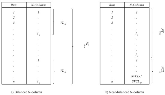
Figure 1.
Structure of a balanced and a near-balanced N-column.
For a given N-column, where NTN value is the ratio of n with respect to the number of levels in the column (ln) (see Equation (11)). If NTN is integer the vector complementary levels does not exist and the column is balanced, in the other case; the column is near-balanced and the vector of complementary levels exists.
The size of the vector of complementary levels for a column near-balanced is SVCLN, defined in the Equation (12).
Then, VCLN = [1:SVCLN]T.
2.2. Method to Build a NONBPA
This section shows the NONBPA method see Figure 2. The method consists in 3 steps described below.
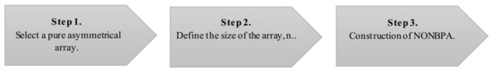
Figure 2.
NONBPA method.
Step 1. Select a pure asymmetrical array. Select a mixed-level design in which factor levels are not multiples of each other.
Step 2. Define the size of the array, n. Determine n ensuring that this is equal or greater to the necessary degrees of freedom needed. For example, for a design with 4 qualitative factors with 5, 6, 7, and 9 levels, the minimum degrees of freedom required to estimate all effects are: 4 + 5 + 6 + 8 (main effects) + 1 (intercept) + 1 (error) = 25, the smallest fraction that can be constructed is size 25.
Step 3. Construction of NONBPA. For the ith factor, replicate the vector 1, …, li (with li, the number of levels) until n runs have been assembled. The last vector can be completed (balanced column) or cut before being completed (near-balanced column).
Example, Construction of NONBPA (24,516171)
Consider a situation that involves three qualitative factors: A, B, and C with 5, 6, and 7 levels, respectively. The experimenter is interested in running a fraction, given that factor levels are not multiple of each other, he decides to use the NONBPA method. Figure 3 shows step by step the construction of a NONBPA.
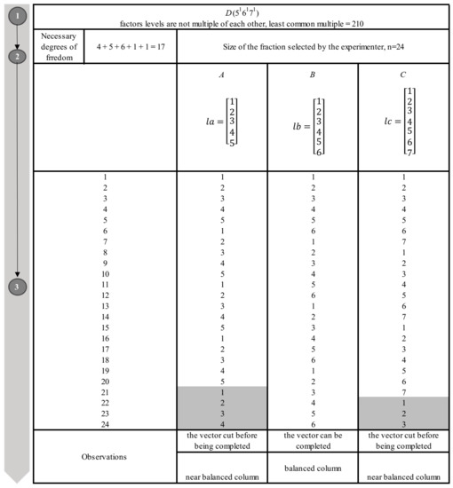
Figure 3.
Construction of NONBPA (24,516171).
In step 1, the design selected is the D(516171). In Step 2, the size of the array is determined by the experimenter, in this case, a size of 24 was chosen, n = 24. Step 3 consists in the construction of array. First, we will mention column B, note that last vector can be completed, therefore the column is balanced. For columns A and C, the last vector is cut before being completed, for this reason columns A and C are near-balanced.
If the experimenter is interested in keeping a specific factor balanced, this can be done by changing the size of the array. Table 4 shows several possibilities of n for this design. Note that to preserve the balance property, it is advisable to select an array size that is a multiple of la × lb …. × ln, where la, lb …. ln are the levels of the factors we want to be balanced in the fraction. This table can also be useful to select n, for example, n = 30, keeps factors A and B balanced while maintaining a reasonable fraction size.
Table 4.
Several possibilities of size fraction for D(516171) with qualitative factors.
Figure 4 shows the GBM calculation for the design (315171) note that the column of factor B is a balanced column. Therefore, Hjt = 0. That is, all the levels for this column appear with the same frequency Ctj = [4,4,4,4,4,4]T. On the other hand, since columns A and C are semi-balanced, they have values of Hjt > 0. That is, they have a contribution of 0.8 and 1.71 respectively and GBM = 0.80 + 0 + 1.71 = 2.51. Regarding orthogonality, J2 =112 while = 1.01. Therefore, NONBPA (516171) is a semi-orthogonal array in which the predictors are minimally correlated.
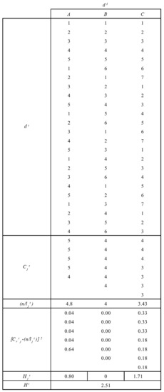
Figure 4.
Calculated GBM for NONBPA (24,516171).
2.3. Augmentation Strategies vs. NONBPAs
Ghosh and Rao (1996) presented a comprehensive study on sequential assembly of fractions (see Figure 5) [33]. They used the design presented by Box [34] (p. 394), this design is presented in T1; it contains 7 factors and 8 runs. T2 is obtained from T1 by switching the signs of column 4. T3 is obtained from T1 by switching the signs of all columns and T4 is presented as T2 with the columns (1,2,3) as (4, 5, 6), (4, 5, 6) as (1,2,3) and the runs (rows) are also in different order. T4 is known as a Search Design [35]. Then a series of augmentation options are presented and evaluated in terms of balance and orthogonality.
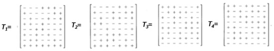
Figure 5.
Sequential assembly of fraction.
The coincidence between these matrices and the NONBPAs is notable. Because in the NONBPAs in a similar way; when renaming the levels of one or more factors it is possible to construct a new fraction. Original NONBPAs and new NONBPAs whit renamed levels have similar properties for balance and orthogonality. Figure 6 shows the level rotation of factor B of NONBPA (213151), note that two additional designs have been generated.
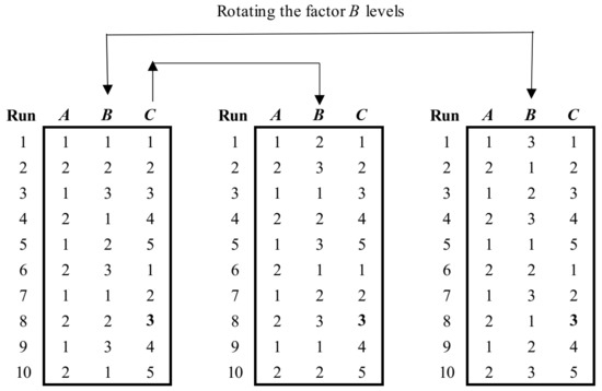
Figure 6.
Level rotation for factor B of NONBPA(213151).
NONBPAs, like many other designs can be augmented. In this section we show a simple strategy to augment the NONBPAs with M additional new runs determined by the experimenter. To increase a NONBPA, it is enough to decide M and then to add the M additional rows by rotating factor levels.
Example, Augmenting a NONBPA (15,21315171111) with 7 Additional Runs
Figure 7 shows a NONBPA (15,21315171111) augmented with M = 7 additional runs. Note that the first 15 runs belong to the original NONBPA and the new M = 7 runs are added by rotating factor levels. Note that creating a NONBPA of size n + M from scratch would produce the same fraction.
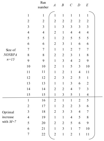
Figure 7.
NONBPA (15,21315171111) augmented with 7 runs.
Table 5 shows a comparison between the NONBPA (15,516171) and its augmented versions. In both designs the number of balanced columns is 2. Increasing the number of runs directly benefits columns A and E, minimally effects B and C and has no effect on D. This provoked a significant reduction in the GBM value from 3.90 to 2.72 improving the balance. Regarding the orthogonality property, the values of J2 and were calculated; as it is already known, J2 increases as the number of runs increases. Therefore, a direct comparison is not possible. A direct comparison is achieved with the ; from 1.03 to 1.01, note that the design becomes more orthogonal as the number of runs increases.
Table 5.
Properties NONBPA (15,516171) vs. NONBPA augmented (21,516171).
3. Results Comparison of NONBPAs vs. EAs
NONBPAs were compared with its competitors, the EAs, presented in [3]. To perform the comparison, four EAs were selected, including EA(21,314171), EA(20,314151), EA(24,516171), and EA(15,21315171). The equivalent NONBPAs were constructed and augmented so that the number of runs of the NONBPAs were equal to the number of runs of the EAs. In this way, a more direct comparison was possible. To compare the designs, the balance (GBM) and orthogonality (J2 and ) are measured. Figure 8 and Figure 9 show that the EAs and the NONBPAs have similar levels for balance and orthogonality, the difference is only minimal only with respect to values. It was also observed that GBM and J2 remain equal for EAs and NONBPAs even if the size of the array changes. Figure 10 shows an efficient array for a D(315171) compared to its corresponding NONBPA. The comparison was made by using 15, 21, and 30 runs. Note that in all cases, the GBM and the J2 were identical for EAs and NONBPAs, and values are very similar.

Figure 8.
Comparison of EAs vs. NONBPAs for the (21,314171) and (20,314151).
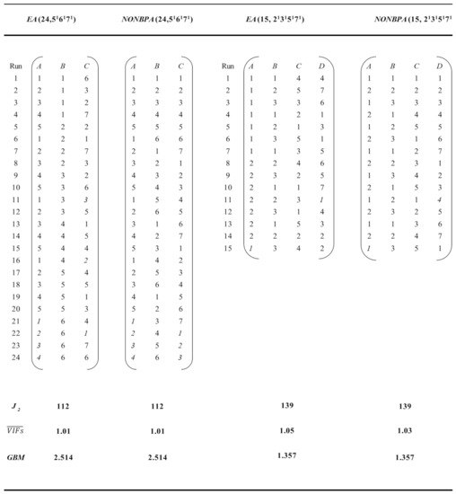
Figure 9.
Comparison of EAs vs. NONBPAs for the (24,516171) and (20,21315171).
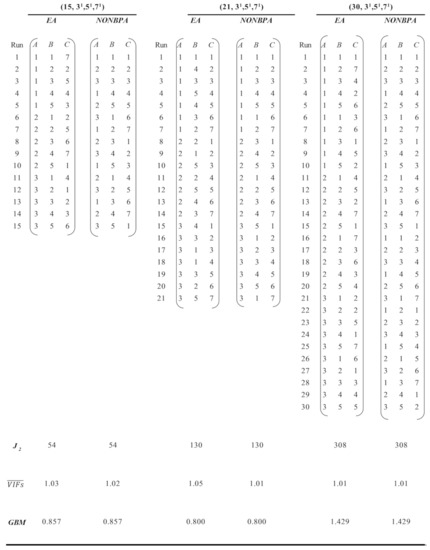
Figure 10.
Comparison of EA vs. NONBPA using different run size.
4. Practical Application
To demonstrate de capacity of the NONBPAs to estimate factorial effects, the method was compared to full factorial and EA using simulated data (Figure 11). The design selected to perform the comparisons was the D(210,21315171). To generate the simulated data, a simple model with the form Y = 6 [A] + 10 [C] + ε(0, σ2), was used and an experimental error was introduced, which is a random variable with zero mean (u = 0) and variance (σ2) [27]. Based on research performed by Ríos et al. (2011), the size of the variance must be one third of the regression coefficient for the regressor to be reported as significant [23].
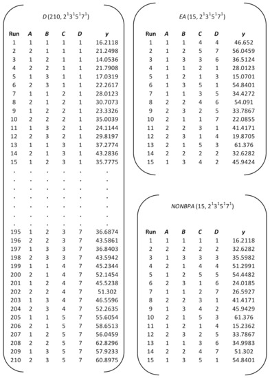
Figure 11.
Simulated data for full factorial, EA and NONBPA.
Table 6 shows the ANOVA tables and the optimization for the three designs. Results are very consistent for the three methods; ANOVA tables look similar, and all the designs were able to detect A and C as significant effects. Regarding the optimization, a desirability function for maximization was used and the three designs produced the same recommended levels for factors A and C, which are two and five, respectively. In all cases, the optimal value for the response is very similar.
Table 6.
ANOVA tables and optimization for full factorial, EA, and NONBPA.
5. Conclusions
Industrial experiments often involve situations in which categorical and numerical factors with different numbers of levels are present, these experiments are commonly known as mixed-level designs. Mixed-level designs require a high number of runs and are difficult to carry out because of the cost and time required. One alternative to avoid running a full factorial is to run a mixed-level fractional factorial design. Unfortunately, these fractions are not easy to construct because they often require complex programming techniques, specialized software, and expensive computer equipment.
The new method presented here, called NONBPA, is an algorithm capable of generating mixed-level fractional factorial designs when the factor levels are not multiple of each other. The near-orthogonal near-balanced pure symmetrical arrays generated are extremely flexible in run size and possess high levels of balance and orthogonality. The arrays generated with this method were compared to the EAs presented in [3] and the results showed that the balance and orthogonality property were identical for both methods. In addition to the construction method, a method to perform augmentations was also provided, this method allows augmenting any NONBPA with M additional runs while preserving the balance and orthogonality properties.
The main advantages of the NONBPA method are that it is easy to understand and apply, it does not require complex programming, the computational cost is low and it can be used by any person with basic knowledge in statistics.
GBM and are parameters that allow to compare respectively, balance and orthogonality between arrays with the same or different number of runs. On the other hand, J2 only allows the comparison of the level of orthogonality between arrays that have same number of runs. A disadvantage in the use of J2 for NONBPAs is that it is not possible to know the minimum value of L(n) for semi-orthogonal arrays. Therefore, for the NONBPAs the use of is recommended.
Future research for the NONBPA will focus on evaluating balance and orthogonality beyond main effects, opening a greater number of possibilities for experimenters in the various fields of application.
Author Contributions
Conceptualization, Y.V.P.-P.; methodology, Y.V.P.-P. and A.J.R.-L.; validation, Y.V.P.-P. and A.J.R.-L., J.A.V.-L. and J.A.J.-G.; formal analysis, Y.V.P.-P.; investigation, Y.V.P.-P., A.J.R.-L., J.A.V.-L., J.A.J.-G., M.L.A.-E. and M.T.-E.; writing—original draft preparation, Y.V.P.-P., A.J.R.-L., M.L.A.-E. and M.T.-E.; writing—review and editing, Y.V.P.-P., A.J.R.-L. All authors have read and agreed to the published version of the manuscript.
Funding
This research received no external funding.
Institutional Review Board Statement
Not applicable.
Informed Consent Statement
Not applicable.
Data Availability Statement
Not applicable.
Acknowledgments
We thank the editor and reviewers for their helpful comments and suggestion that greatly improved the content and quality of paper.
Conflicts of Interest
The authors declare no conflict of interest.
Abbreviations
| Notation | Interpretation |
| NOBA | Near-orthogonal balanced array |
| NONBPA | Near-balanced pure asymmetrical array |
| d | Design matrix |
| n | Number of runs (rows) of d |
| k | Number of factors (columns) of d |
| , sk | Number of levels in the column |
| M | Additional runs in a design |
| EA | Efficient array |
| GBM | General balanced metric |
| J2 | Orthogonal parameter |
| VIF | Variance inflation factors |
| Average variance inflation factors | |
| GMA | Generalized minimum aberration |
| MMA | Minimum moment aberration |
| MAP | Moment aberration projection |
| Balance coefficient | |
| L(n) | The minimum value that is reached by J2 when a matrix is orthogonal |
| CV | Common variance |
| Rj2 | Coefficient of determination of the regression |
| NTN | Number of times the VLN |
| VLN | Vector of levels for the N-factor |
| VCLN | The vector of complementary levels for the N-factor |
| SVCLN | The size of the vector of complementary levels for a column near-balanced |
References
- Wilkie, D. A method of analysis of mixed level factorial experiments. Appl. Stat. 1962, 11, 184. [Google Scholar] [CrossRef]
- Hedayat, A.S.; Sloane, N.J.A.; Stufken, J. Orthogonal Arrays: Theory and Applications; Springer: New York, NY, USA, 1999; Available online: https://www.springer.com/gp/book/9780387987668 (accessed on 27 February 2021).
- Guo, Y.; Simpson, J.R.; Pignatiello, J.J. Construction of efficient mixed-level fractional factorial designs. J. Qual. Technol. 2007, 39, 241–257. [Google Scholar] [CrossRef]
- Schoen, E.D.; Eendebak, P.T.; Nguyen, M.V.M. Complete enumeration of pure-level and mixed-level orthogonal arrays. Wiley Intersci. 2009, 18, 13–140. [Google Scholar] [CrossRef]
- Liu, M.; Fang, K.; Hickernell, F.J. Connections among different criteria for asymmetrical fractional factorial designs. Stat. Sin. 2006, 16, 1285–1297. Available online: http://www.jstor.org/stable/24307788 (accessed on 30 December 2020).
- Fang, K.T.; Ge, G.N.; Liu, M.Q.; Quin, H. Construction of minimum generalized aberration designs. Metrika 2003, 57, 37–50. [Google Scholar] [CrossRef]
- Xu, H. An algorithm for constructing orthogonal and nearly-orthogonal arrays with mixed levels and small runs. Technometrics 2002, 44, 356–368. [Google Scholar] [CrossRef]
- Guo, Y.; Simpson, J.R.; Pignatiello, J.J. The general balance metric for mixed-level fractional factorial designs. Qual. Reliab. Int. 2009, 25, 335–344. [Google Scholar] [CrossRef]
- Wang, J.C.; Wu, C.F.J. An approach to the construction of asymmetrical orthogonal designs. J. Am. Stat. Assoc. 1991, 86, 450–456. [Google Scholar] [CrossRef]
- Wang, J.C.; Wu, C.F.J. Nearly orthogonal arrays with mixed levels and small runs. Technometrics 1992, 34, 409–422. [Google Scholar] [CrossRef]
- Wang, J.C. Mixed difference matrices and the construction of orthogonal arrays. Stat. Probab. Lett. 1996, 28, 121–126. [Google Scholar] [CrossRef]
- Fontana, R. Algebraic generation of minimum size orthogonal fractional factorial designs: An approach based on integer linear programming. Comput. Stat. 2013, 28, 241–253. [Google Scholar] [CrossRef]
- Fontana, R. Generalized minimum aberration mixed-level orthogonal arrays: A general approach based on sequential integer quadratically constrained quadratic programming. Commun. Stat. Theory Methods 2017, 46, 4275–4284. [Google Scholar] [CrossRef][Green Version]
- Grömping, U.; Fontana, R. An algorithm for generating good mixed-level factorial designs. Phys. Chem. 2018, 137, 101–114. [Google Scholar] [CrossRef]
- Xu, H.; Wu, C.F.J. Generalized minimum aberration for asymmetrical fractional factorial designs. Ann. Stat. 2001, 29, 549–560. Available online: http://www.jstor:stable/2674070 (accessed on 10 October 2020).
- Xu, H. Minimum moment aberration for nonregular designs and supersaturated designs. Stat. Sin. 2003, 3, 691–708. [Google Scholar]
- Xu, H.; Deng, L.Y. Moment aberration projection for nonregular fractional factorial designs. Technometrics 2005, 47, 121–131. Available online: https://www.jstor:stable/25470974 (accessed on 10 October 2020). [CrossRef][Green Version]
- Guo, Y.; Simpson, J.R.; Pignatiello, J.J. Deciphering all those minimum aberration criteria for experimental designs. Qual. Eng. 2009, 21, 432–445. [Google Scholar] [CrossRef]
- Nguyen, N.K. A Note on the construction of Near- Orthogonal designs with mixed levels and economic run size. Technometrics 1996, 38, 279–283. [Google Scholar] [CrossRef]
- Lee, K.; Lee, K.; Han, S. Use of an orthogonal array based on the Kriging model to maximize the fatigue life of a turbine blade. Int. J. Struct. Integr. 2011, 2, 303–312. [Google Scholar] [CrossRef]
- Dean, A.; Lewis, S. Methods for Experimentation in Industry, Drug Discovery and Generics; Springer: Secaucus, NJ, USA, 2006; Available online: https://www.springer.com/gp/book/9780387280134 (accessed on 27 February 2021).
- Guo, Y.; Simpson, J.R.; Pignatiello, J.J. Optimal foldover plans for mixed-level fractional factorial designs. Qual. Reliab. Int. 2009, 25, 449–466. [Google Scholar] [CrossRef]
- Ríos, A.J.; Simpson, J.R.; Guo, Y. Semifold plans for mixed designs. Qual. Reliab. Int. 2011, 27, 921–929. [Google Scholar] [CrossRef]
- Pantoja, Y.V.; Rios, A.J.; Tapia Esquivias, M. A method for construction of mixed-level fractional designs. Qual. Reliab. Eng. Int. 2019, 35, 1646–1665. [Google Scholar] [CrossRef]
- DeCock, D.; Stufken, J. On finding mixed orthogonal designs of strength 2 with many 2-level factors. Stat. Probab. Lett. 2000, 50, 383–388. [Google Scholar] [CrossRef]
- Salawu, I.S.; Adele BLOyeyemi, G.M. J2 optimality and Multi-level Minimum Aberration Criteria in fractional factorial design. J. Nat. Sci. Res. 2012, 2, 69–76. [Google Scholar]
- Montgomery, D.C. Design and Analysis of Experiments, 9th ed.; Wiley and Sons Inc.: Hoboken, NJ, USA, 2017. [Google Scholar]
- Li, W.; Lin, D.K.J. Optimal Foldover Plans for Two-Level Fractional Factorial Designs. Technometrics 2003, 45, 142–149. Available online: https://www.jstor:stable/25047011 (accessed on 30 October 2020). [CrossRef]
- Montgomery, D.C.; Runger, G.C. Foldovers of 2k-p resolution IV experimental design. J. Qual. Technol. 1996, 28, 446–450. [Google Scholar] [CrossRef]
- Ghosh, S.; Chowdhury, S. CV, ECV, and Robust CV designs for replications under a class of linear models in factorial experiments. J. Stat. Plan. Inference 2017, 188, 1–7. [Google Scholar] [CrossRef]
- Vu, D.H.; Muttaqi, K.M.; Agalgaonkar, A.P. A variance inflation factor and backward elimination based robust regression model for forecasting monthly electricity demand using climatic variables. Appl. Energy 2015, 140, 385–394. [Google Scholar] [CrossRef]
- Alin, A. Multicollinearity. Wiley Interdiscip. Rev. Comput. Stat. 2010, 2, 370–374. [Google Scholar] [CrossRef]
- Ghosh, S.; Rao, C.R. Handbook of Statistics 13 Design and Analysis of Experiments; Elsevier Science Pub Co.: North Holland, The Netherlands, 1996; Available online: https://www.sciencedirect.com/handbook/handbook-of-statistics/vol/13 (accessed on 27 February 2021).
- Box, G.E.P.; Hunter, W.G.; Hunter, J.S. Statistic for Experiments: An Introduction to Design. In Data Analysis, and Model Building; Wiley: New York, NY, USA, 1978. [Google Scholar]
- Srivastava, J.N. Design for searching non-negligible effects. In A Survey of Statistical Design and Linear Models; North-Holland: Amsterdam, The Netherlands, 1975; pp. 507–519. [Google Scholar]
Publisher’s Note: MDPI stays neutral with regard to jurisdictional claims in published maps and institutional affiliations. |
© 2021 by the authors. Licensee MDPI, Basel, Switzerland. This article is an open access article distributed under the terms and conditions of the Creative Commons Attribution (CC BY) license (https://creativecommons.org/licenses/by/4.0/).