The Asymptotic Expansion of a Function Introduced by L.L. Karasheva

Abstract

The asymptotic expansion for $x\to \pm \infty$ of the entire function $F_{n,\sigma }(x;\mu )={\displaystyle \sum _{k=0}^{\infty }}\frac{sin\left(n{\gamma }_k\right)}{sin{\gamma }_k}\frac{x^k}{k!\mathsf{\Gamma }(\mu -\sigma k)},$ ${\gamma }_k=\frac{(k+1)\pi }{2n}$ for $\mu >0$, $0<\sigma <1$ and $n=1,2,\dots$ is considered. In the special case $\sigma =\alpha /\left(2n\right)$, with $0<\alpha <1$, this function was recently introduced by L.L. Karasheva (J. Math. Sciences, 250 (2020) 753–759) as a solution of a fractional-order partial differential equation. By expressing $F_{n,\sigma }(x;\mu )$ as a finite sum of Wright functions, we employ the standard asymptotics of integral functions of hypergeometric type to determine its asymptotic expansion. This was found to depend critically on the parameter $\sigma$ (and to a lesser extent on the integer n). Numerical results are presented to illustrate the accuracy of the different expansions obtained.

1. Introduction

In a recent paper, L.L. Karasheva [1] introduced the entire function

$${\mathsf{\Theta }}_{n,\alpha }(x;\mu ):=\sum _{k=0}^{\infty }\frac{sin\left(n{\gamma }_k\right)}{sin{\gamma }_k}\frac{x^k}{k!\mathsf{\Gamma }(\mu -\frac{\alpha k}{2n})},{\gamma }_k:=\frac{(k+1)\pi }{2n},$$

(1)

where $\mu >0$, $0<\alpha <1$ and $n=1,2,\dots$ and, throughout, x is a real variable. This function is of interest as it is involved in the fundamental solution of the differential equation

$$\frac{{\partial }^{\alpha }u}{\partial t^{\alpha }}+{(-1)}^n\frac{{\partial }^{2n}u}{\partial x^{2n}}=f(x,t)$$

for positive integer n, where the derivative with respect to t is the fractional derivative of the order $\alpha$. In the simplest case $n=1$, we have ${\mathsf{\Theta }}_{1,\alpha }(x;\mu )=\varphi (-\sigma ,\mu ;x)$, $\sigma :=\alpha /\left(2n\right)$, where $\varphi (-\sigma ,\mu ;x)$ is the Wright function

$$\varphi (-\sigma ,\mu ;x):=\sum _{k=0}^{\infty }\frac{x^k}{k!\mathsf{\Gamma }(\mu -\sigma k)}(\sigma <1),$$

(2)

which finds application as a fundamental solution of the diffusion-wave equation [2]. Under the above assumptions on n and $\alpha$ it follows that the parameter $\sigma$ associated with (1) satisfies $0<\sigma <\frac{1}{2}$.

In this study, however, we shall allow the parameter $\sigma$ to satisfy $0<\sigma <1$ and consider the function

$$F_{n,\sigma }(x;\mu ):=\sum _{k=0}^{\infty }\frac{sin\left(n{\gamma }_k\right)}{sin{\gamma }_k}\frac{x^k}{k!\mathsf{\Gamma }(\mu -\sigma k)}(0<\sigma <1),$$

(3)

which coincides with ${\mathsf{\Theta }}_{n,\alpha }(x;\mu )$ when $\sigma =\alpha /\left(2n\right)$. From the well-known expansion

$$\frac{sin\left(n{\gamma }_k\right)}{sin{\gamma }_k}=\sum _{r=0}^{n-1}{e}^{i{\gamma }_k(2r-n+1)}=\sum _{r=0}^{n-1}{e}^{-i(k+1){\omega }_r},$$

where

$${\omega }_r:=\frac{(n-2r-1)\pi }{2n}(0\le r\le n-1),$$

(4)

it follows that (3) can be expressed as a finite sum of Wright functions defined in (2) with rotated arguments (compare [1], Equation (4))

$$F_{n,\sigma }(x;\mu )=\sum _{r=0}^{n-1}{e}^{-i{\omega }_r}\varphi (-\sigma ,\mu ;x{e}^{-i{\omega }_r}).$$

(5)

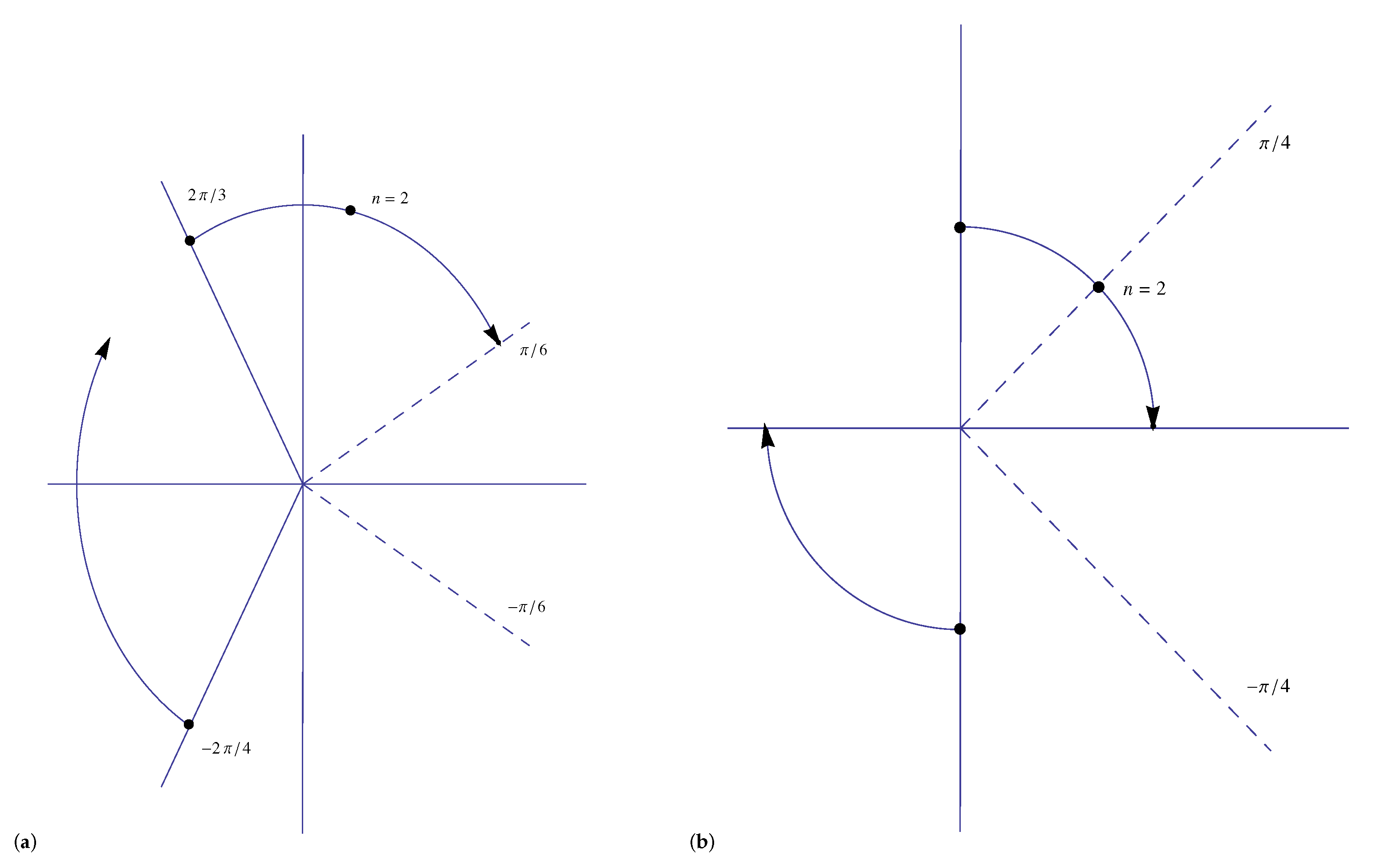
We note that the extreme values of ${\omega }_r$ satisfy ${\omega }_0=-{\omega }_{n-1}=(n-1)\pi /\left(2n\right)$, whence $|{\omega }_r|<\frac{1}{2}\pi$ for $0\le r\le n-1$.

We use the representation in (5), with the values of ${\omega }_r$ in (4), to determine the asymptotic expansion of $F_{n,\sigma }(x;\mu )$ for $x\to \pm \infty$ by application of the asymptotic theory of the Wright function. A summary of the expansion of $\varphi (-\sigma ,\mu ;z)$ for large $\left|z\right|$ is given in Section 3. The expansions of $F_{n,\sigma }(x;\mu )$ for $x\to \pm \infty$ are given in Section 4 and Section 5, where they are shown to depend critically on the parameter $\sigma$ (and to a lesser extent on the integer n). A concluding section presents our numerical results confirming the accuracy of the different expansions obtained.

2. An Alternative Representation of ${\mathit{F}}_{\mathit{n},\mathit{\sigma }}(\mathit{x};\mathit{\mu })$

The Wright function appearing in (2) can be written alternatively as

$$\varphi (-\sigma ,\mu ;x)=\frac{1}{\pi }\sum _{k=0}^{\infty }\frac{x^k}{k!}\mathsf{\Gamma }(1-\mu +\sigma k)sin\pi (\mu -\sigma k)$$

$$=\frac{1}{2\pi }\left\{e^{\pi i\vartheta }\mathsf{\Psi }\left(x{e}^{\pi i\sigma }\right)+e^{-\pi i\vartheta }\mathsf{\Psi }\left(x{e}^{-\pi i\sigma }\right)\right\}$$

upon use of the reflection formula for the gamma function, where $\vartheta :=\frac{1}{2}-\mu$. The associated Wright function $\mathsf{\Psi }\left(z\right)$ is defined by

$$\mathsf{\Psi }\left(z\right):=\sum _{k=0}^{\infty }\frac{z^k}{k!}\mathsf{\Gamma }(\sigma k+\delta )(0<\sigma <1,\delta =1-\mu ),$$

(6)

which is valid for $\left|z\right|<\infty$. Hence, we obtain the representation

$$F_{n,\sigma }(x;\mu )=\frac{1}{2\pi }\sum _{r=0}^{n-1}{e}^{-i{\omega }_r}{{\rm Y}}_r(\sigma ;x),$$

where

$${{\rm Y}}_r(\sigma ;x):=e^{\pi i\vartheta }\mathsf{\Psi }\left(x{e}^{\pi i\sigma -i{\omega }_r}\right)+e^{-\pi i\vartheta }\mathsf{\Psi }\left(x{e}^{-\pi i\sigma -i{\omega }_r}\right).$$

If we now exploit the symmetry of the ${\omega }_r$ in (4) (and the fact that x is a real variable), we observe that the values of ${\omega }_r$ for $0\le r\le N-1$, where $N=\lfloor n/2\rfloor$, satisfy

$$\{{\omega }_0,{\omega }_1,\dots ,{\omega }_{N-1}\}=\left\{\frac{(n-1)\pi }{2n},\frac{(n-3)\pi }{2n},\dots ,\frac{\pi }{2n}{ϵ}_n\right\},{ϵ}_n=\left\{\begin{array}{cc}1\hfill & \left(n\mathrm{even}\right)\hfill \\ 2\hfill & \left(n\mathrm{odd}\right).\hfill \end{array}\right.$$

(7)

Then, we can write

$${\mathrm{F}}_{n,\sigma }(x;\mu )=\frac{1}{\pi }\Re \left\{\sum _{r=0}^{N-1}{e}^{-i{\omega }_r}{{\rm Y}}_r(\sigma ;x)+{\Delta }_n{e}^{\pi i\vartheta }\mathsf{\Psi }\left(x{e}^{\pi i\sigma }\right)\right\},$$

(8)

where

$${\Delta }_n=\left\{\begin{array}{cc}0\hfill & \left(n\mathrm{even}\right)\hfill \\ 1\hfill & \left(n\mathrm{odd}\right).\hfill \end{array}\right.$$

The form (8) involves half the number of Wright functions $\mathsf{\Psi }\left(z\right)$ and will be used to determine the asymptotic expansion of $F_{n,\sigma }(x;\mu )$ as $x\to \pm \infty$ in Section 4 and Section 5.

3. The Asymptotic Expansion of $\mathsf{\Psi }\left(\mathit{z}\right)$ for $\left|\mathit{z}\right|\to \infty$

We first present the large-$\left|z\right|$ asymptotics of the function $\mathsf{\Psi }\left(z\right)$ in (6) based on the presentation described in ([3], Section 4); see also ([4], Section 4.2), ([5], §2.3). We introduce the following parameters:

$$\kappa =1-\sigma ,h={\sigma }^{\sigma },\vartheta =\delta -\frac{1}{2},\delta =1-\mu ,$$

(9)

together with the associated (formal) exponential and algebraic expansions

$$E\left(z\right):=Z^{\vartheta }{e}^Z\sum _{j=0}^{\infty }{A}_j\left(\sigma \right)Z^{-j},H\left(z\right):=\frac{1}{\sigma }\sum _{k=0}^{\infty }\frac{{(-1)}^k}{k!}\mathsf{\Gamma }\left(\frac{k+\delta }{\sigma }\right)z^{-(k+\delta )/\sigma },$$

(10)

where (The dependence of the coefficients $A_j\left(\sigma \right)$ on the parameter $\delta$ is not indicated.)

$$Z:=\kappa {\left(hz\right)}^{1/\kappa },A_0\left(\sigma \right)={(2\pi /\kappa )}^{1/2}{(\sigma /\kappa )}^{\vartheta }.$$

(11)

Then, since $0<\kappa <1$, we obtain from ([5], p. 57) the large-z expansion

$$\mathsf{\Psi }\left(z\right)\sim \left\{\begin{array}{cc}E\left(z\right)+H\left(z{e}^{\mp \pi i}\right)\hfill & \left(\right|argz|\le \frac{1}{2}\pi \kappa )\hfill \\ \\ H\left(z{e}^{\mp \pi i}\right)\hfill & (\frac{1}{2}\pi \kappa <|argz|\le \pi ),\hfill \end{array}\right.$$

(12)

where the upper or lower signs are chosen according as $argz>0$ or $argz<0$, respectively.

The expansion $E\left(z\right)$ is exponentially large as $\left|z\right|\to \infty$ in the sector $|argz|<\frac{1}{2}\pi \kappa$, and oscillatory (multiplied by the algebraic factor $z^{\vartheta /\kappa }$) on the anti-Stokes lines $argz=\pm \frac{1}{2}\pi \kappa$. In the adjacent sectors $\frac{1}{2}\pi \kappa <|argz|<\pi \kappa$, the expansion $E\left(z\right)$ continues to be present, but is exponentially small reaching maximal subdominance relative to the algebraic expansion on the Stokes lines (On these rays, $E\left(z\right)$ undergoes a Stokes phenomenon where it switches off in a smooth manner (see [6], p. 67).) $argz=\pm \pi \kappa$. In our treatment of $F_{n,\sigma }(x;\mu )$, we will not be concerned with exponentially small contributions, except in one special case when $x\to -\infty$ where the expansion of $F_{n,\sigma }(x;\mu )$ is exponentially small.

The first few normalised coefficients $c_j=A_j\left(\sigma \right)/A_0\left(\sigma \right)$ are [3,4]:

$$\begin{array}{c}{c}_0=1,c_1=\frac{1}{24\sigma }\{2+7\sigma +2{\sigma }^2-12\delta (1+\sigma )+12{\delta }^2\},\\ c_2=\frac{1}{1152{\sigma }^2}\{4+172\sigma +417{\sigma }^2+172{\sigma }^3+4{\sigma }^4-24\delta (6+41\sigma +41{\sigma }^2+6{\sigma }^3)+120{\delta }^2(4+11\sigma +4{\sigma }^2)-480{\delta }^3(1+\sigma )+144{\delta }^4\},\\ c_3=\frac{1}{414,720{\sigma }^3}\left\{\right(-1112+9636\sigma +163,734{\sigma }^2+336,347{\sigma }^3+163,734{\sigma }^4+9636{\sigma }^5-1112{\sigma }^6)-\delta (3600+220,320\sigma +929,700{\sigma }^2+929,700{\sigma }^3+220,320{\sigma }^4+3600{\sigma }^5)+{\delta }^2(65,520+715,680\sigma +1,440,180{\sigma }^2+715,680{\sigma }^3+65,520{\sigma }^4)-{\delta }^3(161,280+816,480\sigma +816,480{\sigma }^2+161,280{\sigma }^3)+{\delta }^4(151,200+378,000\sigma +151,200{\sigma }^2)-60,480{\delta }^5(1+\sigma )+8640{\delta }^6\}.\end{array}$$

(13)

In addition to the Stokes lines $argz=\pm \pi \kappa$, where $E\left(z\right)$ is maximally subdominant relative to the algebraic expansion, the positive real axis is also a Stokes line. Here, the algebraic expansion is maximally subdominant relative to $E\left(z\right)$. As the positive real axis is crossed from the upper to the lower half plane the factor $e^{-\pi i}$ appearing in $H\left(z{e}^{-\pi i}\right)$ changes to $e^{\pi i}$, and vice versa. The details of this transition will not be considered here; see ([5], p. 248) for the case of the confluent hypergeometric function ${}_1{F}_1(a;b;z)$.

4. The Asymptotic Expansion of ${\mathit{F}}_{\mathit{n},\mathit{\sigma }}(\mathit{x};\mathit{\mu })$ for $\mathit{x}\to +\infty$

4.1. Asymptotic Character as a Function of $\sigma$

Let us denote the arguments of the $\mathsf{\Psi }$ functions appearing in (8) by

$$z_r^{\pm }=xexp\left[i{\varphi }_r^{\pm }\right],{\varphi }_r^{\pm }=\pm \pi \sigma -{\omega }_r.$$

The representation of the asymptotic structure of the functions $\mathsf{\Psi }\left(z_r^{\pm }\right)$ is illustrated in Figure 1 for different values of $\sigma$. The figures show the rays $argz=\pm \pi \sigma$ and the anti-Stokes lines (dashed lines) $argz=\pm \frac{1}{2}\pi \kappa$. In the case $\sigma =\frac{2}{3}$, the exponentially large sector is $|argz|<\frac{1}{6}\pi$, and it is seen from Figure a that the arguments $z_r^{\pm }$ for $0\le r\le N-1$ and $x{e}^{\pm \pi i\sigma }$ all lie in the domain where $\mathsf{\Psi }\left(z\right)$ has an algebraic expansion; this conclusion applies a fortiori when $\frac{2}{3}<\sigma <1$. When $\sigma =\frac{1}{2}$, the exponentially large sector is $|argz|<\frac{1}{4}\pi$; when $n=2$, we have ${\omega }_0=\frac{1}{4}\pi$ so that $z_0^{+}$ is situated on the boundary of the exponentially large sector.

Figure 1. Diagrams representing the rays $argz=\pm \pi \sigma$ and the boundaries of the exponentially large sector (shown by dashed rays) $|argz|<\frac{1}{2}\pi \kappa$, $\kappa =1-\sigma$ for (a) $\sigma =2/3$, (b) $\sigma =1/2$, (c) $\sigma =1/3$, and (d) $\sigma =1/6$. Outside the exponentially large sector, the expansion of $\mathsf{\Psi }\left(z\right)$ is algebraic in character. The circular quadrants represent the range of the arguments $argz=\pm \pi \sigma -{\omega }_r$ for $0\le r\le \lfloor n/2\rfloor -1$, with $n\ge 2$ and the arrow-head corresponds to $n=\infty$. When $\sigma =1/3$, the rays $argz=\pm \pi \sigma$ and $argz=\pm \frac{1}{2}\pi \kappa$ coincide.

Other values of $n\ge 3$ will have some $z_r^{+}$ inside this sector, whereas the $z_r^{-}$ are in the algebraic sector for $n\ge 2$. Similarly, the case $\sigma =\frac{1}{3}$, where the rays $argz=\pm \pi \sigma$ and $argz=\pm \frac{1}{2}\pi \kappa$ coincide, has all the $z_r^{+}$ situated in the exponentially large sector, with the $z_r^{-}$ situated in the algebraic domain. Finally, when $\sigma =\frac{1}{6}$, the exponentially large sector $|argz|<\frac{5}{12}\pi$ encloses the rays $argz=\pm \pi \sigma$ with the result that all the $z_r^{+}$ lie in the exponentially large sector, whereas the $z_r^{-}$ lie in the algebraic domain (except when $n=2$ when $z_0^{-}$ lies on the lower boundary of the exponentially large sector).

To summarise, we have the following asymptotic character of $F_{n,\sigma }(x;\mu )$ when $x\to +\infty$ as a function of the parameter $\sigma$:

$$\left.\begin{array}{cc}0<\sigma <\frac{1}{2}\hfill & \mathrm{Exp}.\mathrm{large}+\mathrm{Algebraic}(\mathrm{for}n\ge 2)\hfill \\ \\ \frac{1}{2}\le \sigma <\frac{2}{3}\hfill & \mathrm{Exp},\mathrm{large}\left(\mathrm{dependent}\mathrm{on}n\right)+\mathrm{Algebraic}\hfill \\ \\ \frac{2}{3}\le \sigma <1\hfill & \mathrm{Algrbraic}(\mathrm{for}n\ge 2).\hfill \end{array}\right\}$$

(14)

4.2. Asymptotic Expansion

From (8) and (10), we have the algebraic expansion associated with $F_{n,\sigma }(x;\mu )$ given by

$$\mathbf{H}\left(x\right)=\frac{1}{\sigma }\sum _{k=0}^{\infty }\frac{x^{-K}}{k!\mathsf{\Gamma }(1-K)}{\theta }_{n,k},K:=\frac{k+\delta }{\sigma },$$

(15)

where, with appropriate choices of the factors $e^{\pm \pi i}$ in $H\left(z\right)$,

$$\begin{array}{ccc}\hfill {\theta }_{n,k}& =& \frac{{(-1)}^k}{sin\pi K}\Re \{{\displaystyle \sum _{r=0}^{N-1}}{e}^{\pi i\vartheta -i{\omega }_r}{(e^{\pi i\sigma -i{\omega }_r}·e^{-\pi i})}^{-K}+e^{-\pi i\vartheta -i{\omega }_r}{(e^{-\pi i\sigma -i{\omega }_r}·e^{\pi i})}^{-K}\hfill \\ & & +{\Delta }_n{e}^{\pi i\vartheta }{(e^{\pi i\sigma }·e^{-\pi i})}^{-K}\}\hfill \\ & =& \frac{{(-1)}^k}{sin\pi K}\Re \left\{{\displaystyle \sum _{r=0}^{N-1}}{e}^{(K-1)i{\omega }_r}(e^{\pi i(\vartheta +\kappa K)}+e^{-\pi i(\vartheta +\kappa K)})+{\Delta }_n{e}^{\pi i(\vartheta +\kappa K)}\right\}\hfill \\ & =& \Re \left\{2{\displaystyle \sum _{r=0}^{N-1}}{e}^{(K-1)i{\omega }_r}+{\Delta }_n\right\},\hfill \end{array}$$

(16)

as $cos\pi (\vartheta +\kappa K)=cos\pi (K-k-\frac{1}{2})={(-1)}^{k}sin\pi K$.

For the exponential component, we introduce the quantities

$$X=\kappa {\left(hx\right)}^{1/\kappa },{\mathsf{\Phi }}_r^{\pm }=\pm \frac{\pi \vartheta }{\kappa }-{\omega }_r\left(1+\frac{\vartheta }{\kappa }\right)$$

(17)

and the formal asymptotic sum

$$S\left(X{e}^{i\Omega }\right):=\sum _{j=0}^{\infty }{A}_j\left(\sigma \right){\left(X{e}^{i\Omega /\kappa }\right)}^{-j}.$$

(18)

Then, from (8) and (10), we have the exponential expansion in the form

$$\mathbf{E}\left(x\right)=\frac{X^{\vartheta }}{\pi }\Re \{\sum _{r=0}^{N-1}\left(exp[X{e}^{i{\varphi }_r^{+}/\kappa }+i{\mathsf{\Phi }}_r^{+}]S\left(X{e}^{i{\varphi }_r^{+}}\right)+exp[X{e}^{i{\varphi }_r^{-}/\kappa }+i{\mathsf{\Phi }}_r^{-}]S\left(X{e}^{i{\varphi }_r^{-}}\right)\right)$$

$$+{\Delta }_{n}exp[X{e}^{\pi i\sigma /\kappa }+\pi i\vartheta /\kappa ]S\left(X{e}^{\pi i\sigma }\right)\}.$$

(19)

It is important to stress that only the exponential terms with $|{\varphi }_r^{\pm }|\le \frac{1}{2}\pi \kappa$, that is those with

$$|\pm \pi \sigma -{\omega }_r|\le \frac{1}{2}\pi \kappa ,$$

are to be retained in $\mathbf{E}\left(x\right)$ in (19). In addition, it is seen by inspection of Figure 1 that the second term involving $S\left(X{e}^{i{\varphi }_r^{-}}\right)$ does not contribute to $\mathbf{E}\left(x\right)$ when $\frac{1}{3}\le \sigma <1$, since, for this range of $\sigma$, the ray $argz=-\pi \sigma$ lies outside (or, when $\sigma =\frac{1}{3}$, on the lower boundary of) the exponentially large sector $|argz|<\frac{1}{2}\pi \kappa$. Thus, when $\frac{1}{2}\le \sigma <\frac{2}{3}$, the exponential expansion is significant if $\pi \sigma -{\omega }_0\le \frac{1}{2}\pi \kappa$; that is, if $n\ge n_0=1/(2-3\sigma )$.

In summary, we have the following theorem.

Theorem 1.

The following expansion holds for $x\to +\infty$:

$$F_{n,\sigma }(x;\mu )\sim \left\{\begin{array}{cc}\mathbf{E}\left(x\right)+\mathbf{H}\left(x\right)\hfill & (0<\sigma <\frac{1}{2};n\ge 2)\hfill \\ \\ \mathbf{E}\left(x\right)+\mathbf{H}\left(x\right)\hfill & (\frac{1}{2}\le \sigma <\frac{2}{3};n\ge n_0)\hfill \\ \\ \mathbf{H}\left(x\right)\hfill & (\frac{1}{2}\le \sigma <\frac{2}{3};n<n_0)\hfill \\ \\ \mathbf{H}\left(x\right)\hfill & (\frac{2}{3}\le \sigma <1;n\ge 2),\hfill \end{array}\right.$$

where $n_0=1/(2-3\sigma )$ and the exponential and algebraic expansions $\mathbf{E}\left(x\right)$ and $\mathbf{H}\left(x\right)$ are defined in (15) and (19).

4.3. Karasheva’s Estimate for $|{\mathsf{\Theta }}_{n,\alpha }(x;\mu )|$

When $\sigma =\alpha /\left(2n\right)<\frac{1}{2}$, we see from Theorem 1 that the dominant exponential expansion as $x\to +\infty$ corresponds to $r=0$, yielding

$${\mathsf{\Theta }}_{n,\alpha }(x;\mu )\sim \frac{A_0\left(\sigma \right)X^{\vartheta }}{\pi }\Re exp\left[X{e}^{i(\pi \sigma -{\omega }_0)/\kappa +i{\mathsf{\Phi }}_0^{+}}\right]$$

$$=\frac{A_0\left(\sigma \right)X^{\vartheta }}{\pi }exp[Xcos(\pi \sigma -{\omega }_0)/\kappa )]cos[Xsin(\pi \sigma -{\omega }_0)/\kappa )+{\mathsf{\Phi }}_0^{+}],$$

where

$$\frac{\pi \sigma -{\omega }_0}{\kappa }=\frac{2n\pi \sigma -(n-1)\pi }{2n-\alpha }=\frac{(\alpha +1-n)\pi }{2n-\alpha }.$$

Thus, we have the leading order estimate

$${\mathsf{\Theta }}_{n,\alpha }(x;\mu )\sim \frac{A_0\left(\sigma \right)X^{\vartheta }}{\pi }exp\left[Xcos\left(\frac{(n-1-\alpha )\pi }{2n-\alpha }\right)\right]cos\left[Xsin\left(\frac{(n-1-\alpha )\pi }{2n-\alpha }\right)-{\mathsf{\Phi }}_0^{+}\right]$$

(20)

as $x\to +\infty$. When expressed in our notation, Karasheva’s estimate for $|{\mathsf{\Theta }}_{n,\alpha }(x;\mu )|$ in ([1], §8) agrees with (20) (when the second cosine term is replaced by 1), except that she did not give the value of the multiplicative constant $A_0\left(\sigma \right)/\pi$ given in (11). However, the presentation of her result as an upper bound is not evident due to the presence of possibly less dominant exponential expansions and also the subdominant algebraic expansion.

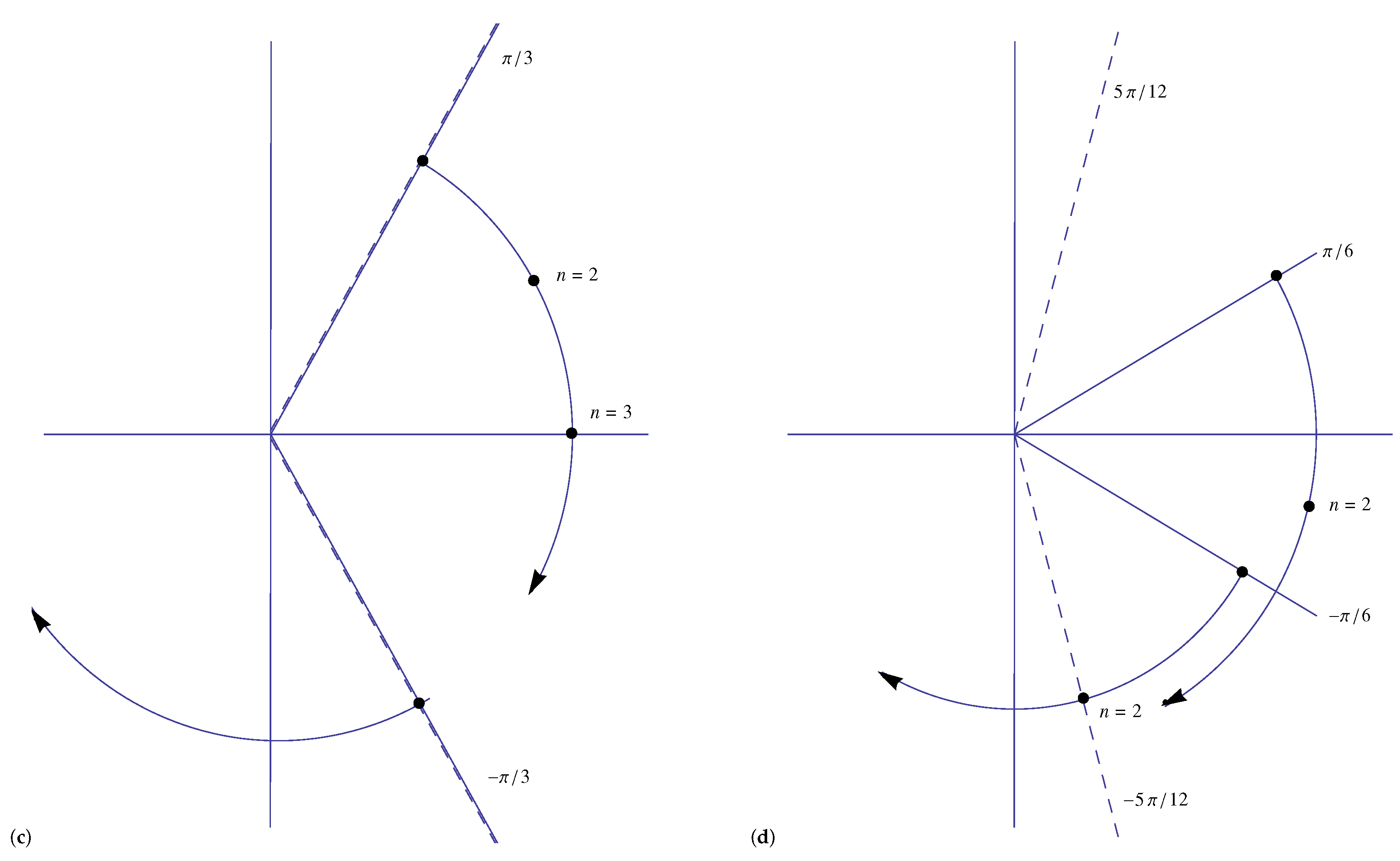
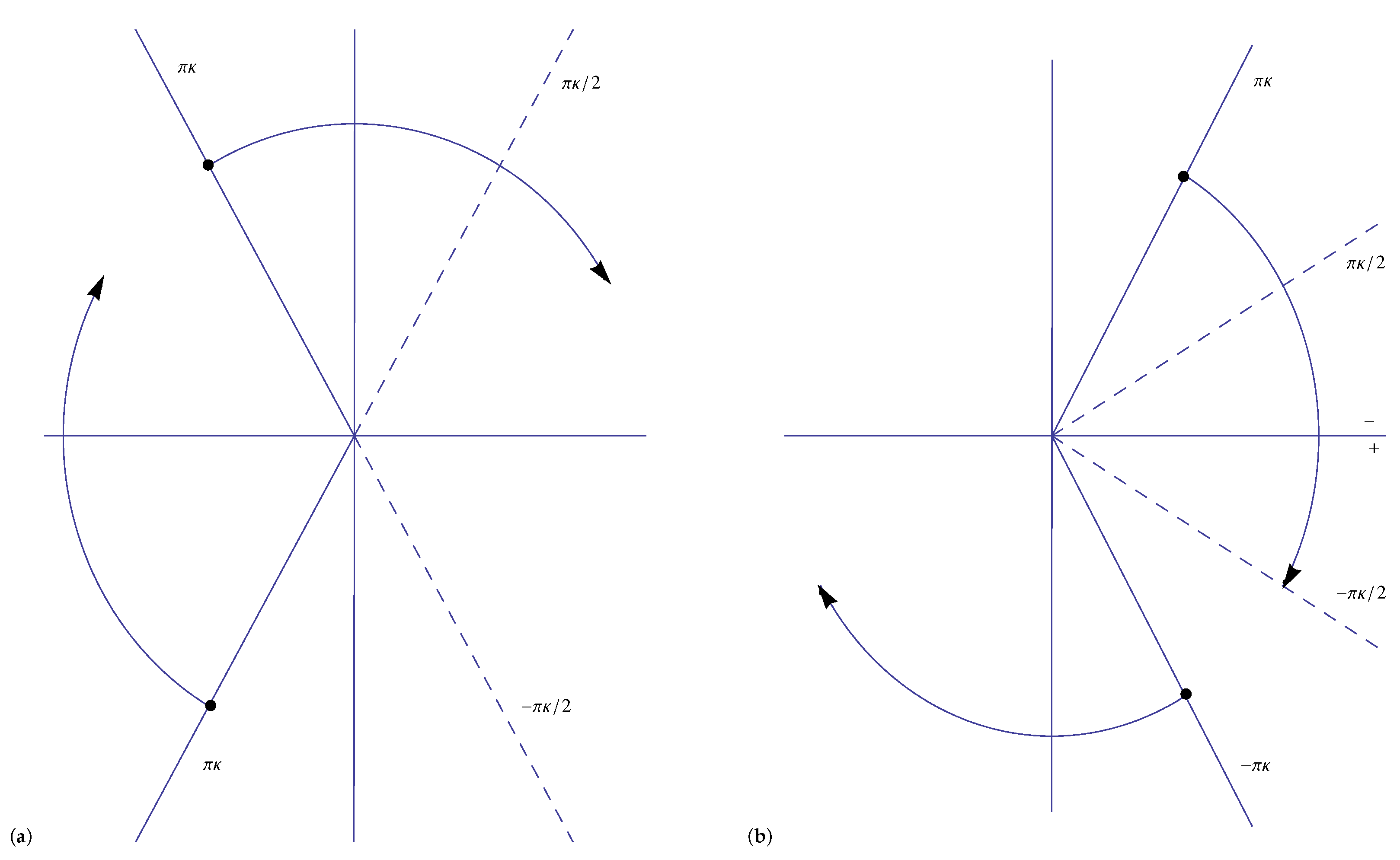
5. The Expansion of ${\mathit{F}}_{\mathit{n},\mathit{\sigma }}(\mathit{x};\mathbf{\mu })$ for $\mathbf{x}\to -\infty$

To examine the case of negative x, we replace x by $e^{\mp \pi i}x$, with $x>0$, and use the fact that $\mathsf{\Psi }\left(z{e}^{2\pi i}\right)=\mathsf{\Psi }\left(z\right)$ to find, from (8), that

$$F_{n,\sigma }(-x;\mu )=\frac{1}{\pi }\Re \left\{\sum _{r=0}^{N-1}{e}^{-i{\omega }_r}{{\rm Y}}_r(-\kappa ;x)+{\Delta }_n{e}^{\pi i\vartheta }\mathsf{\Psi }\left(x{e}^{-\pi i\kappa }\right)\right\}.$$

(21)

The rays $argz=\pm \pi \sigma$ in Figure 1 are now replaced by the Stokes lines $argz=\pm \pi \kappa$. The Stokes and anti-Stokes lines $argz=\pm \frac{1}{2}\pi \kappa$ are illustrated in Figure 2 when $0<\sigma <\frac{1}{2}$ and $\frac{1}{2}<\sigma <1$. In the sectors $\frac{1}{2}\pi \kappa <|argz|<\pi \kappa$, we recall that the exponential expansion $E\left(z\right)$ is still present but is exponentially small as $\left|z\right|\to \infty$.

Figure 2. Diagrams representing the rays $argz=\pm \pi \kappa$ and the boundaries of the exponentially large sector (shown by dashed rays) $|argz|<\frac{1}{2}\pi \kappa$, $\kappa =1-\sigma$ for (a) $0<\sigma <\frac{1}{2}$ and (b) $\frac{1}{2}<\sigma <1$. The circular quadrants represent the range of the arguments $argz=\pm \pi \kappa -{\omega }_r$ for $0\le r\le N-1$ with the arrow-head corresponding to $n=\infty$. The ± signs in (b) denote the signs to be chosen in $H\left(z\right)$ on either side of the Stokes line $argz=0$.

For the algebraic component of the expansion two cases arise when the argument $\pi \kappa -{\omega }_r$ of the second $\mathsf{\Psi }$ function in ${{\rm Y}}_r(-\kappa ;x)$ is either (i) positive or (ii) negative. In case (i), the algebraic expansion $H\left(z\right)$ does not encounter a Stokes phenomenon as its argument does not cross $argz=0$, whereas in case (ii), a Stokes phenomenon arises for those values of r that make $\pi \kappa -{\omega }_r<0$. In case (i), the algebraic component contains the factor inside the sum over r in (21)

$$e^{\pi i\vartheta }{(e^{-\pi i\kappa -i{\omega }_r}·e^{\pi i})}^{-K}+e^{-\pi i\vartheta }{(e^{\pi i\kappa -i{\omega }_r}·e^{-\pi i})}^{-K}$$

$$=e^{i{\omega }_{r}K}(e^{\pi i(\vartheta -\sigma K)}+e^{-\pi i(\vartheta -\sigma K)})=2e^{i{\omega }_{r}K}cos\pi (k+\frac{1}{2})\equiv 0$$

upon recalling the definition of K in (15) and noting that $\delta -\vartheta =\frac{1}{2}$. Similarly, the final term involves the factor $\Re e^{\pi i\vartheta }{(e^{-\pi i\kappa }·e^{\pi i})}^{-K}=cos\pi (\vartheta -\sigma K)=0$. Thus, the algebraic contribution to $F_{n,\sigma }(-x;\mu )$ vanishes in case (i).

For case (ii) to apply, we require that $\pi \kappa -{\omega }_0<0$; that is, $n>n^{*}=1/(2\sigma -1)$. Suppose that $\pi \kappa -{\omega }_r<0$ for $0\le r\le r_0$. Then, the algebraic component resulting from the terms with $r\le r_0$ becomes

$$\frac{1}{\pi \sigma }\Re \left\{\sum _{k=0}^{\infty }\frac{{(-1)}^k\mathsf{\Gamma }\left(K\right)}{k!}{x}^{-K}\sum _{r=0}^{r_0}{e}^{(K-1)i{\omega }_r}\left(e^{\pi i\vartheta }{(e^{-\pi i\kappa }·e^{\pi i})}^{-K}+e^{-\pi i\vartheta }{(e^{\pi i\kappa }·e^{\pi i})}^{-K}\right)\right\}$$

$$=\frac{2}{\pi \sigma }\Re \left\{\sum _{k=0}^{\infty }\frac{{(-1)}^k\mathsf{\Gamma }\left(K\right)}{k!}{x}^{-K}\sum _{r=0}^{r_0}{e}^{(K-1)i{\omega }_r-\pi iK}cos\pi (\vartheta -\sigma K+\pi K)\right\},$$

where, in the second term in round braces, we have taken account of the Stokes phenomenon (the first term and that multiplied by ${\Delta }_n$ are unaffected). Some routine algebra then produces the algebraic contribution

$$\widehat{\mathbf{H}}\left(x\right):=\frac{2}{\sigma }\sum _{k=0}^{\infty }\frac{x^{-K}}{k!\mathsf{\Gamma }(1-K)}{\widehat{\theta }}_{n,k},{\widehat{\theta }}_{n,k}:=\sum _{r=0}^{r_0}cos\left\{\pi K-(K-1){\omega }_r\right\}$$

(22)

when $n>n^{*}$ and $\widehat{\mathbf{H}}\left(x\right)\equiv 0$ when $n<n^{*}$. (We avoid here consideration of the algebraic contribution when $\pi \kappa -{\omega }_r=0$, that is, on the Stokes line $argz=0$.)

Reference to Figure 2 shows that there is no exponential contribution to $F_{n,\sigma }(-x;\mu )$ from the terms $\mathsf{\Psi }\left(x{e}^{-\pi i\kappa }\right)$ and $\mathsf{\Psi }\left(x{e}^{-\pi i\kappa -i{\omega }_r}\right)$. From (10) and (21), we find the exponential expansion results from the terms $\mathsf{\Psi }\left(x{e}^{\pi i\kappa -i{\omega }_r}\right)$, which is given by

$$\widehat{\mathbf{E}}\left(x\right):=\frac{X^{\vartheta }}{\pi }\Re \sum _{r=0}^{N-1}exp[-X{e}^{-i{\omega }_r/\kappa }-i\mathsf{\Phi }]S(-X{e}^{-i{\omega }_r/\kappa }),$$

(23)

where X and the asymptotic sum S are defined in (17) and (18) with $\mathsf{\Phi }:={\omega }_r(1+\vartheta /\kappa )$. For $\sigma <\frac{1}{2}$ (when the algebraic expansion vanishes), the expansion of $F_{n,\sigma }(-x;\mu )$ will be exponentially small provided $\pi \kappa -{\omega }_0>\frac{1}{2}\pi \kappa$; that is, when $n<1/\sigma$. If $n=1/\sigma$, there is an exponentially oscillatory contribution, and when $n>1/\sigma$, the expansion is exponentially large.

To summarise, we have the theorem:

Theorem 2.

The following expansion holds for $x\to +\infty$:

$$F_{n,\sigma }(-x;\mu )\sim \left\{\begin{array}{cc}\widehat{\mathbf{E}}\left(x\right)\hfill & (0<\sigma \le \frac{1}{2})\hfill \\ \\ \widehat{\mathbf{E}}\left(x\right)+\widehat{\mathbf{H}}\left(x\right)\hfill & (\frac{1}{2}<\sigma <1),\hfill \end{array}\right.$$

(24)

where the exponential expansion $\widehat{\mathbf{E}}\left(x\right)$ is defined in (23). This last expansion is exponentially small as $x\to -\infty$ when $0<\sigma <\frac{1}{2}$ and $n<1/\sigma$. The algebraic expansion $\widehat{\mathbf{H}}\left(x\right)$ is given by

$${\displaystyle \widehat{\mathbf{H}}\left(x\right):=\frac{2}{\sigma }\sum _{k=0}^{\infty }\frac{x^{-K}}{k!\mathsf{\Gamma }(1-K)}{\widehat{\theta }}_{n,k}(n>n^{*}),0(n<n^{*}),}$$

where $n^{*}=1/(2\sigma -1)$ and K, ${\widehat{\theta }}_{n,k}$ are specified in (15) and (22).

6. Numerical Results

In this section, we describe numerical calculations that support the expansions given in Theorems 1 and 2. The function $F_{n,\sigma }(x;\mu )$ was evaluated using the expression in terms of Wright functions (valid for real x)

$$F_{n,\sigma }(x;\mu )=2\Re \sum _{r=0}^{N-1}{e}^{i{\omega }_r}\varphi (-\sigma ,\mu ;x{e}^{i{\omega }_r})+{\Delta }_n\varphi (-\sigma ,\mu ;x),N=\lfloor n/2\rfloor ,$$

(25)

which follows from (5) and the symmetry of ${\omega }_r$.

In Table 1, we present the results of numerical calculations for $x\to +\infty$ compared with the expansions given in Theorem 1. We choose four representative values of $\sigma$ that focus on the different cases of Theorem 1 and $n=2,3$ and 4. The numerical value of $F_{n,\sigma }(x;\mu )$ was obtained by high-precision evaluation of (25). The exponential expansion $\mathbf{E}\left(x\right)$ was computed with the truncation index $j=3$ and the algebraic expansion $\mathbf{H}\left(x\right)$ was optimally truncated (that is, at or near its smallest term).

Table 1. The values of the exponential and algebraic expansions compared with $F_{n,\sigma }(x;\mu )$ for large $x>0$ for different values of $\sigma$ and n when $\mu =3/4$ and $x=8$.

$\mathbf{\sigma }$		$\mathbf{n}=\mathbf{2}$	$\mathbf{n}=\mathbf{3}$	$\mathbf{n}=\mathbf{4}$
1/3	$\mathbf{E}\left(x\right)$	$-1.81418881\times {10}^2$	$-1.08294258\times {10}^3$	$-3.08231679\times {10}^3$
	$\mathbf{H}\left(x\right)$	$+0.34241316$	$+0.17280892$	$+0.34497729$
	$\mathbf{E}\left(x\right)+\mathbf{H}\left(x\right)$	$-1.81076468\times {10}^2$	$-1.08276977\times {10}^3$	$-3.08197181\times {10}^3$
	$F_{n,\sigma }(x;\mu )$	$-1.80709370\times {10}^2$	$-1.08284759\times {10}^3$	$-3.08254767\times {10}^3$
1/2	$\mathbf{E}\left(x\right)$	$+0.06317153$	$+1.15957937\times {10}^3$	$-4.47945373\times {10}^4$
	$\mathbf{H}\left(x\right)$	$+0.74012019$	$+1.09449277$	$+1.45169481$
	$\mathbf{E}\left(x\right)+\mathbf{H}\left(x\right)$	$+0.80329172$	$+1.16067387\times {10}^3$	$-4.47930856\times {10}^4$
	$F_{n,\sigma }(x;\mu )$	$+0.80329527$	$+1.16069221\times {10}^3$	$-4.47921506\times {10}^4$
5/9	$\mathbf{E}\left(x\right)$	$--$	$-0.14805870$	$+2.77243091\times {10}^2$
	$\mathbf{H}\left(x\right)$	$+0.79825166$	$+1.17615555$	$+1.55857242$
	$\mathbf{E}\left(x\right)+\mathbf{H}\left(x\right)$	$+0.79825166$	$+1.02809685$	$+2.78801663\times {10}^2$
	$F_{n,\sigma }(x;\mu )$	$+0.79825119$	$+1.02809649$	$+2.78801134\times {10}^2$
2/3	$\mathbf{H}\left(x\right)$	$+0.84046066$	$+1.23266920$	$+1.63072031$
	$F_{n,\sigma }(x;\mu )$	$+0.84046066$	$+1.23266920$	$+1.63072031$

The first case $\sigma =\frac{1}{3}$ has an exponentially large expansion with a subdominant algebraic contribution for all three values of n. The second case $\sigma =\frac{1}{2}$ corresponds to $n_0=2$; when $n=2$, $\mathbf{E}\left(x\right)$ is oscillatory and makes a similar contribution as $\mathbf{H}\left(x\right)$, whereas when $n=3$ and 4, $\mathbf{E}\left(x\right)$ is exponentially large. The third case $\sigma =\frac{5}{9}$ corresponds to $n_0=3$; when $n=2$, there is no exponential contribution, whereas when $n=3$, $\mathbf{E}\left(x\right)$ is oscillatory and thus makes a similar contribution as $\mathbf{H}\left(x\right)$; when $n=4$, $\mathbf{E}\left(x\right)$ is exponentially large. Finally, when $\sigma =\frac{2}{3}$, the expansion of $F_{n,\sigma }(x;\mu )$ is purely algebraic in character.

In Table 2, we present illustrative examples of Theorem 2 when $x\to -\infty$. The first case, $\sigma =\frac{1}{4}$ ($\kappa =\frac{3}{4}$), has an expansion that is exponential in character; for $n<1/\sigma =4$, $\widehat{\mathbf{E}}\left(x\right)$ is exponentially small, whereas for $n=4$, the argument $\pi \kappa -{\omega }_0=\frac{3}{8}\pi$ lies on the upper boundary of the exponentially large sector $|argz|<\frac{3}{8}\pi$, and thus $\widehat{\mathbf{E}}\left(x\right)$ is oscillatory. For $n\ge 5$, $\widehat{\mathbf{E}}\left(x\right)$ becomes exponentially large as $x\to -\infty$. In the second case, $\sigma =\frac{2}{5}$ ($\kappa =\frac{3}{5}$), $\widehat{\mathbf{E}}\left(x\right)$ is exponentially small for $n=2$ and exponentially large for $n\ge 3$.

Table 2. The values of the exponential and algebraic expansions compared with $F_{n,\sigma }(x;\mu )$ for large $x<0$ for different values of $\sigma$ and n when $\mu =3/4$ and $\left|x\right|=8$ (for $\sigma =1/4,1/2,2/5$), $\left|x\right|=5$ (for $\sigma =3/4$).

$\mathit{\sigma }$		$\mathit{n}=2$	$\mathit{n}=3$	$\mathit{n}=4$
1/4	$\widehat{\mathbf{E}}\left(x\right)$	$+1.59003829\times {10}^{-2}$	$+1.77442984\times {10}^{-1}$	$+6.49578248\times {10}^{-1}$
	$F_{n,\sigma }(-x;\mu )$	$+1.59003416\times {10}^{-2}$	$+1.77011100\times {10}^{-1}$	$+6.49580223\times {10}^{-1}$
2/5	$\widehat{\mathbf{E}}\left(x\right)$	$-4.18901636\times {10}^{-2}$	$-3.79446870\times {10}^0$	$-3.02428770\times {10}^1$
	$F_{n,\sigma }(-x;\mu )$	$-4.18889220\times {10}^{-2}$	$-3.79475882\times {10}^0$	$-3.02402120\times {10}^1$
1/2	$\widehat{\mathbf{E}}\left(x\right)$	$-0.56022532$	$+1.23070020\times {10}^3$	$-1.28808653\times {10}^4$
	$F_{n,\sigma }(-x;\mu )$	$-0.56023534$	$+1.23066913\times {10}^3$	$-1.28803505\times {10}^4$
3/4	$\widehat{\mathbf{E}}\left(x\right)$	$+1.81213632\times {10}^{28}$	$+7.55354383\times {10}^{13}$	$-0.84956415$
	$\widehat{\mathbf{H}}\left(x\right)$	$--$	$-1.93112636\times {10}^{-1}$	$-0.28756658$
	$\widehat{\mathbf{E}}\left(x\right)+\widehat{\mathbf{H}}\left(x\right)$	$+1.81213632\times {10}^{28}$	$+7.55354383\times {10}^{13}$	$-1.13713072$
	$F_{n,\sigma }(-x;\mu )$	$+1.81213650\times {10}^{28}$	$+7.55354314\times {10}^{13}$	$-1.13713081$

In the third case, $\sigma =\kappa =\frac{1}{2}$, $\widehat{\mathbf{E}}\left(x\right)$ is oscillatory for $n=2$ and exponentially large for $n\ge 3$. Finally, when $\sigma =\frac{3}{4}$ ($\kappa =\frac{1}{4}$), the function $F_{n,\sigma }(x;\mu )$ is exponentially large for $n=2,3$ and $n\ge 5$. However, for $n=4$, the two values ${\omega }_0=\frac{3}{8}\pi$ and ${\omega }_1=\frac{1}{8}\pi$ yield arguments $\pi \kappa -{\omega }_r$ ($r=0,1$) situated on both boundaries of the exponentially large sector $|argz|<\frac{1}{8}\pi$. In this case $\widehat{\mathbf{E}}\left(x\right)$ is oscillatory and, since $n^{*}=2$, there is, in addition, an algebraic contribution $\widehat{\mathbf{H}}\left(x\right)$.

7. Concluding Remarks

We employed the standard asymptotics of the Wright function $\mathsf{\Psi }\left(z\right)$ defined in (6) to determine the asymptotic expansion of $F_{n,\sigma }(x;\mu )$ for $x\to \pm \infty$. We found that this behaviour depended critically on the parameter $\sigma$. The numerical results presented in Table 1 and Table 2 demonstrate that the asymptotic forms of $F_{n,\sigma }(x;\mu )$ stated in Theorems 1 and 2 agreed well with the numerically computed values of $F_{n,\sigma }(\pm x;\mu )$. In particular, we showed that, when $\sigma <\frac{1}{2}$, the expansion of $F_{n,\sigma }(x;\mu )$ exponentially decays as $x\to -\infty$.