A Solution Procedure Combining Analytical and Numerical Approaches to Investigate a Two-Degree-of-Freedom Vibro-Impact Oscillator

Abstract

In this paper, a new approach is proposed to analyze the behavior of a nonlinear two-degree-of-freedom vibro-impact oscillator subject to a harmonic perturbing force, based on a combination of analytical and numerical approaches. The nonlinear governing equations are analytically solved by means of a new analytical technique, namely the Optimal Auxiliary Functions Method (OAFM), which provided highly accurate explicit analytical solutions. Benefiting from these results, the application of Schur principle made it possible to analyze the stability conditions for the considered system. Various types of possible motions were emphasized, taking into account possible initial conditions and different parameters, and the explicit analytical solutions were found to be very useful to analyze the kinetic energy loss, the contact force, and the stability of periodic motions.

1. Introduction

Vibro-impact processes are widely used in mechanical-engineering applications and devices such as hammer-like devices, rotor-casing dynamical systems, wheel–rail interaction of high-speed railway couches, heat exchangers, fuel elements of nuclear reactors, gears, piping systems [1], stiction and electric short circuits of MEMS [2], noise and wear-producing processes, grinding, foraging, drilling, punching, tamping, pile cutting a variety of objects, and vibrating machinery or structures with stops or clearance [3].

Dynamics of vibro-impact systems has received great attention in the last decades. Some numerical or experimental results were obtained, but adequate analytical predictions need to be further studied. For the first time, Masri [4] analyzed the stability of the impact damper by using the perturbation method. The finite-difference method was used by Kobrinski [5], Babitsky [6], Brîndeu [7], and Okolewska et al. [8]. The nonlinear equation of a single-degree-of-freedom oscillator with an impact damper was analyzed approximately using the method of Kryloff and Bogoliuboff by Cronin and Van [9]. Shaw [10] studied the symmetric double-impact motion, both harmonic and subharmonic, by means of a mapping that related conditions at subsequent impacts. A mechanical system with one degree of freedom was investigated by Ivanov [11] using standard Poincare-Bendixon theory, Lyapunov’s second method, and Zhuravlev transformations. The exact solutions of the vibro-impact oscillator with two degrees of freedom, including localized states and their bifurcation structure, were obtained by Aziz et al. [12]. Stability and bifurcation for the unsymmetrical, periodic motion of a horizontal impact oscillator under a periodic excitation were employed through four mappings based on two switch planes by Luo [13]. De Souza and Caldas [14] implemented the Ott–Grebogi–Yorke (OGY) method to stabilize desired unstable periodic orbits by applying a small perturbation on an available control parameter and introducing an impact map for the dynamical variables. Chaos and periodic motion of a cantilever beam system with impacts was found readily by Emans et al. [15]. In addition, nonlinear behavior such as coexistence of attractors was found even at modest oscillation levels during investigations with realistic parameters.

The dynamics of an impact oscillator with viscoelastic and Hertzian contact was examined by Mann et al. [16] using the presence of multiple periodic attractors, subharmonics, quasi-periodic motions, and chaotic oscillations. Avramov [17] considered the forced vibrations of an impact Duffing oscillator using Zhuravlev’s transformation and the multiple-scale method. The stability and bifurcations of periodic vibrations were explored. The control of vibro-impact dynamics of a single-sided Hertzian contact forced oscillator was considered by Bichri et al. [18]. The multiple-scale technique was applied to study the slow dynamic and the frequency-response curves near the primary resonance. Based on Zhuravlev and Ivanov transformations, Grace et al. [19] developed an analytical model of a ship’s roll motion interacting with ice. Extensive numerical simulations were carried out for all initial conditions covered by the ship’s grazing orbit for different values of excitation amplitude and frequency of the external wave roll moment.

Jovic et al. [20] considered the motion trajectory of a vibro-impact system based on the oscillator moving along a rough parabolic line in the vertical plane, under the action of extreme force with nonlinearity of the bond originates of sliding Coulomb’s type friction force. The study of Askari and Tahani [2] was focused on the effect of mechanical shock on dynamic pull-in instability of electrically actuated microbeams through an alternative reduced-order model and using the fourth-order Runge–Kutta method. By setting up a Poincaré map and using a shooting method, Lin et al. [21] obtained a fixed point of periodic motion in the system, period doubling bifurcation, and Hopf bifurcation. The existing and stability conditions of period-1 motion in a single-degree-of-freedom oscillator with double-side constraints were studied by Wang et al. [22]. A smaller shock gap than impact gap could make the periodic motion more stable.

Reboucas et al. [23] examined limitations of the coefficient of restitution model using experimental observations from a simple vibro-impact setup, and the effect of the magnitude response of gap deviation during an experimental sweep. Numerical simulation using Zhuravlev and Ivanov transformations was obtained. A triboelectric energy harvester on a three-degree-of-freedom vibro-impact oscillator was investigated by Fu et al. [24]. The symmetric mass configurations of the oscillator were more beneficial to energy harvesting than the asymmetric cases. Zukovic et al. [25] explored a vibro-impact system consisting of a crank-slider mechanism with one attached oscillator. The cases with an ideal and a non-ideal excitation were analyzed, and analytical and numerical solutions were obtained for the vibrating system with the ideal excitation. For the system with non-ideal excitation, the average value of the frequency was obtained.

The present paper analyzes the motion of a horizontal vibro-impact system with two degrees of freedom in the case when the external coercive force and viscous damping force are known and a periodic vibro-impact model is realized in the system. A variety of possible cases of motion of the vibro-impact system is presented. This process is very complex, and a nonlinear differential equation for one of the masses and a linear differential equation for the other mass is needed in the analysis. It is very difficult to obtain an exact solution for these types of equations, but an analytical approximate solution with a high accuracy will be given by means of OAFM [26,27,28,29,30,31]. The condition for periodic motion is obtained and the stability of periodic motion is studied.

2. Dynamical Model of the Vibro-Impact System

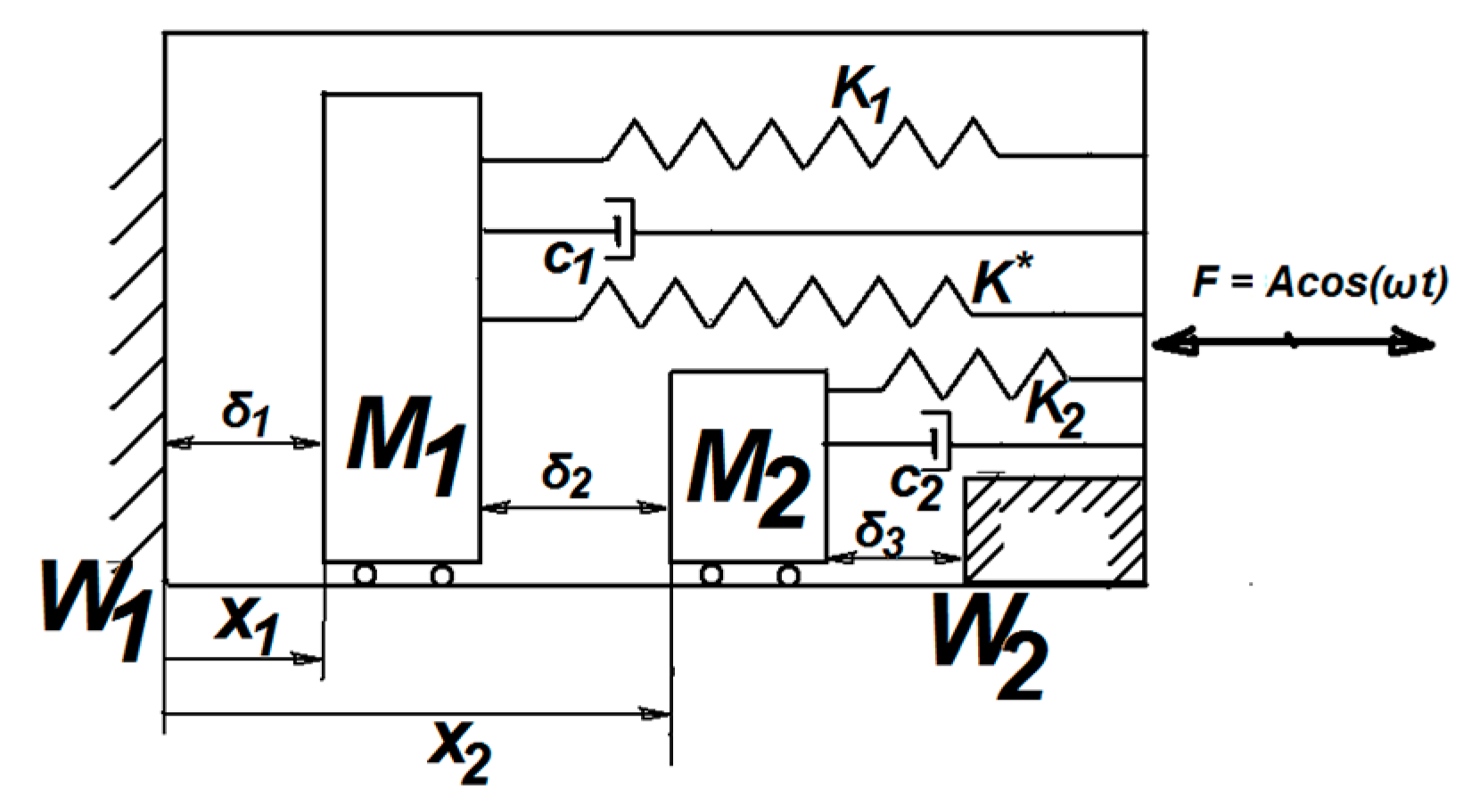
The considered dynamical model of the vibro-impact system under investigation is depicted in Figure 1, which details the two-degree-of-freedom system with gaps.

The system under investigation is composed of a horizontal direction periodical force F = Acosωt and two oscillators of mass M₁ and M₂, which also move in the horizontal direction. These two masses are initially separated by three gaps: δ₁ between the wall W₁ and the mass M₁, δ₂ between the masses M₁ and M₂, and δ₃ between the mass M₂ and the wall W₂. The mass M₁ is connected to a linear spring K₁, nonlinear spring K*, and the damper c₁, and the mass M₂ is connected to linear spring K₂ and damper c₂. The oscillator M₂ collides with the rigid wall W₂ and with the mass M₁. The coefficient of restitution between M₁ and M₂ is R, and R₂ is the coefficient of restitution between M₁ and W₁ and M₂ and W₂. The displacement between the mass M₁ and vertical wall W₁ is x₁, and the displacement between the mass M₂ and the wall W₁ is x₂.

The equations of motion between any two successive collisions are given as:

$$M_1{x^{″}}_1+c_1({x^{\prime }}_1-F^{\prime })+K_1(x_1-F)+K^{*}{(x_1-F)}^3=0,$$

(1)

$$M_2{x^{″}}_2+c_2({x^{\prime }}_2-F^{\prime })+K_2(x_2-F)=0,$$

(2)

where the prime denotes the derivative with respect to time t.

By means of the following transformations:

$$\begin{array}{l}\mathsf{\omega }t=\mathsf{\Omega }\mathsf{\tau }\begin{array}{cc};& {\mathsf{\Omega }}_1={(K_1/M_1)}^{1/2}\end{array}\begin{array}{cc};& {\mathsf{\Omega }}_2=\end{array}(K_2/M_2{)}^{1/2}\begin{array}{cc};& \mathsf{\tau }={\mathsf{\Omega }}_{1}t\end{array}\begin{array}{cc};& x_1={\mathsf{\delta }}_{1}X\end{array}\begin{array}{cc};& x_2={\mathsf{\delta }}_{1}Y\end{array}\begin{array}{cc};& {\mathsf{\alpha }}_1=c_1/(2M_1{\mathsf{\Omega }}_1),\end{array}\\ {\mathsf{\alpha }}_2=c_2/(2M_2{\mathsf{\Omega }}_1);\mathsf{\beta }=K^{*}{\mathsf{\delta }}_1^2/K_1\begin{array}{cc};& a=A/{\mathsf{\delta }}_1\end{array}\begin{array}{cc};& k=\frac{{\mathsf{\Omega }}_2}{{\mathsf{\Omega }}_1}\end{array},\end{array}$$

(3)

Equations (1) and (2) can be rewritten in the dimensionless variables, after some simple manipulations:

$$\ddot{X}+2{\mathsf{\alpha }}_1\dot{X}+\left(1+\frac{3}{2}{a}^2\right)X+\mathsf{\beta }{X}_{}^3=-2{\mathsf{\alpha }}_{1}a\mathsf{\Omega }\sin (\mathsf{\Omega }\mathsf{\tau })+(a+3a\mathsf{\beta }{X}_{}^2+\frac{3}{4}\mathsf{\beta }{a}^3)\cos (\mathsf{\Omega }\mathsf{\tau })-\frac{3}{2}{a}^2\mathsf{\beta }X\cos (2\mathsf{\Omega }\mathsf{\tau })+\frac{\mathsf{\beta }}{4}{a}^3\cos (3\mathsf{\Omega }\mathsf{\tau }),$$

(4)

$$\ddot{Y}+2{\mathsf{\alpha }}_{2}k\dot{Y}+k^{2}Y=a{k}^2\cos (\mathsf{\Omega }\mathsf{\tau })-2{\mathsf{\alpha }}_{2}ka\mathsf{\Omega }\sin (\mathsf{\Omega }\mathsf{\tau }),$$

(5)

where the dot denotes the derivative with respect to variable τ.

Between two successive collisions, the initial conditions of Equations (4) and (5) are:

$$X(0)=1\begin{array}{cc},& \dot{X}\end{array}(0)=V_1\begin{array}{cc},& Y\end{array}(0)=1+\frac{{\mathsf{\delta }}_2}{{\mathsf{\delta }}_1}\begin{array}{cc},& \dot{Y}\end{array}(0)=V_2,$$

(6)

where V₁ and V₂ are known parameters.

Equations (4)–(6) are second-order nonlinear differential equations, and therefore are very difficult to be analytically solved. In the following, we present a relatively new approach, namely the Optimal Auxiliary Functions Method, to obtain an approximate analytical solution in an efficient manner.

3. Basics of the Optimal Auxiliary Functions Method (OAFM)

Following basic concepts of OAFM presented in [26,27,28,29,30,31], in this work, we consider a general nonlinear equation in the form:

$$L[U(\mathsf{\tau })]+N[U(\mathsf{\tau })]=0,$$

(7)

where L and N are the linear differential and nonlinear differential operators, τ is the independent variable, and U(τ) is an unknown function. The initial or boundary conditions are:

$$B\left(U,\frac{dU(\mathsf{\tau })}{d\mathsf{\tau }}\right)=0.$$

(8)

In order to obtain an approximate solution $\overline{U}(\mathsf{\tau })$, we consider that this approximate solution can be expressed in the form:

$$\overline{U}(\mathsf{\tau })=U_0(\mathsf{\tau })+U_1(\mathsf{\tau },C_1,C_2,\dots ,C_n),$$

(9)

in which U₀ (initial approximation) and U₁ (the first approximation) will be determined as described below, and with C₁, C₂,…,C_n being the unknown parameters whose values will be optimally determined.

Substituting Equation (9) into Equation (7), one obtains:

$$L[U_0(\mathsf{\tau })]+L[U_1(\mathsf{\tau })]+N[U_0(\mathsf{\tau })+U_1(\mathsf{\tau },C_1,C_2,\dots ,C_n)]=0.$$

(10)

The initial approximation U₀(τ) can be obtained from the linear equation:

$$L[U_0(\mathsf{\tau })]=0\begin{array}{cc},& B\left(U_0(\mathsf{\tau }),\frac{d{U}_0(\mathsf{\tau })}{d\mathsf{\tau }}\right)=0\end{array},$$

(11)

and therefore, the first approximation is obtained from Equations (10) and (11):

$$L[U_1(\mathsf{\tau },C_1,C_2,\dots ,C_n)]+N[U_0(\mathsf{\tau })+U_1(\mathsf{\tau },C_1,C_2,\dots ,C_n)]=0\begin{array}{cc},& B\left(U_1(\mathsf{\tau }),\frac{d{U}_1(\mathsf{\tau })}{d\mathsf{\tau }}\right)=0\end{array}.$$

(12)

The nonlinear term from Equation (12) can be expanded in the form:

$$N\left[U_0(\mathsf{\tau })+U_1(\mathsf{\tau },C_i)\right]=N[U_0(\mathsf{\tau })]+{\displaystyle \sum _{k=1}^p\frac{U_1^k(\mathsf{\tau },C_i)}{k!}}{N}^{(k)}[U_0(\mathsf{\tau })].$$

(13)

To accelerate the convergence of the first approximation U₁(τ,C_i) and therefore of the approximate solution as well, and also to avoid the difficulties that can appear in solving the nonlinear differential Equation (12), we propose another expression, such that Equation (12) can be written as follows:

$$U_1(\mathsf{\tau },C_1,C_2,\dots ,C_n)+{\displaystyle \sum _{k=1}^n{C}_i{f}_i(\mathsf{\tau })=0}\begin{array}{cc},& B\left(U_1,\frac{\partial U_1}{\partial \mathsf{\tau }}\right)\end{array}=0,$$

(14)

where C_i are arbitrary unknown parameters and f_i(τ) are auxiliary functions depending on the initial approximation U₀(τ), on the functions which appear in N[U(τ)] or N[U₀(τ)] or are combinations of such expressions. These auxiliary functions f_i(τ) are very important and are not unique. It should be emphasized that we have much freedom to choose such auxiliary functions, because it is known that the nonlinear differential equation does not have a unique solution. The parameters C_i, which appear into Equations (9) and (14), can be optimally identified via rigorous methods such as the Galerkin method, the least square method, the Ritz method, the collocation method, or by minimizing the square residual error. In this last case, if:

$$R(\mathsf{\tau },C_i)=L[\overline{U}(\mathsf{\tau })]+N[\overline{U}(\mathsf{\tau })]\begin{array}{cc},& \mathsf{\tau }\in D\end{array},$$

(15)

where $\overline{U}(\mathsf{\tau })$ is given by Equations (9), (11), and (14), then

$$J(C_1,C_2,\dots ,C_n)={\displaystyle \underset{(D)}{\int }{R}^2(\mathsf{\tau },C_i)d\mathsf{\tau }}.$$

(16)

The values of the parameters C_i are obtained from the following system:

$$\frac{\partial J}{\partial C_1}=\frac{\partial J}{\partial C_2}=\dots =\frac{\partial J}{\partial C_n}=0.$$

(17)

It is clear that in this way, the approximate solution $\overline{U}(\mathsf{\tau })$ is well determined after the identification of the optimal values of the initially unknown convergence-control parameters C_i.

4. Application of the Optimal Auxiliary Functions Method to Equations (4)–(6)

The approximate solutions and exact solutions of Equations (4)–(6) are of the following forms:

$$\overline{X}(\mathsf{\tau })=X_0(\mathsf{\tau })+X_1(\mathsf{\tau },C_i)\begin{array}{cc},& i=1,2,\dots ,p\end{array},$$

(18)

$$\overline{Y}(\mathsf{\tau })=Y_0(\mathsf{\tau })+Y_1(\mathsf{\tau },C_i+C_j)\begin{array}{cc},& j=1,2,\dots ,q\end{array}.$$

(19)

For the nonlinear differential Equation (4) and for the linear Equation (5), the linear operators are, respectively:

$$L(X)=\ddot{X}+2{\mathsf{\alpha }}_1\dot{X}+\left(1+\frac{3}{2}{a}^2\right)X,$$

(20)

$$L(Y)=\ddot{Y}+2{\mathsf{\alpha }}_{2}k\dot{Y}+k^{2}Y.$$

(21)

The initial approximations X₀(τ) and the exact solution Y₀(τ) are obtained from the linear equations:

$${\ddot{X}}_0+2{\mathsf{\alpha }}_1{\dot{X}}_0+\left(1+\frac{3}{2}{a}^2\right)X_0=0\begin{array}{cc},& X_0(0)=1\begin{array}{cc},& {\dot{X}}_0(0)=V_1\end{array}\end{array},$$

(22)

$${\ddot{Y}}_0+2{\mathsf{\alpha }}_{2}k{\dot{Y}}_0+k^2{Y}_0=0\begin{array}{cc},& Y_0(0)=1+\frac{{\mathsf{\delta }}_2}{{\mathsf{\delta }}_1}\end{array}\begin{array}{cc},& {\dot{Y}}_0(0)=V_2\end{array},$$

(23)

and therefore:

$$X_0(\mathsf{\tau })=e^{-{\mathsf{\alpha }}_1\mathsf{\tau }}\left(C_1\cos \sqrt{{\overline{\mathsf{\Omega }}}^2-{\mathsf{\alpha }}_1^2}\mathsf{\tau }+C_2\sin \sqrt{{\overline{\mathsf{\Omega }}}^2-{\mathsf{\alpha }}_1^2}\right),{\overline{\mathsf{\Omega }}}^2=1+\frac{3}{2}{a}^2,$$

(24)

$$Y_0(\mathsf{\tau })=e^{-{\mathsf{\alpha }}_{2}k\mathsf{\tau }}\left[C_3\cos \sqrt{k^2-k{\mathsf{\alpha }}_2}\mathsf{\tau }+C_4\sin \sqrt{k^2-k{\mathsf{\alpha }}_2}\mathsf{\tau }\right].$$

(25)

The nonlinear operator for Equation (4) is obtained from Equations (7) and (20):

$$N(X)=\mathsf{\beta }{X}_{}^3+2{\mathsf{\alpha }}_{1}a\mathsf{\Omega }\sin (\mathsf{\Omega }\mathsf{\tau })-(a+3a\mathsf{\beta }{X}_{}^2+\frac{3}{4}\mathsf{\beta }{a}^3)\cos (\mathsf{\Omega }\mathsf{\tau })+\frac{3}{2}{a}^2\mathsf{\beta }X\cos (2\mathsf{\Omega }\mathsf{\tau })-\frac{\mathsf{\beta }}{4}{a}^3\cos (3\mathsf{\Omega }\mathsf{\tau }),$$

(26)

and the corresponding nonlinear operator for Equation (5) is obtained from Equations (7) and (29) as:

$$N(Y)=a{k}^2\cos (\mathsf{\Omega }\mathsf{\tau })-2{\mathsf{\alpha }}_{2}ka\mathsf{\Omega }\sin (\mathsf{\Omega }\mathsf{\tau }).$$

(27)

Taking into account the initial conditions (6) for the first variable X(τ) and the initial conditions for (22) for the initial approximation X₀(τ), one can write the initial conditions for the first approximation X₁(τ):

$$X_1(0)={\dot{X}}_1(0)=0.$$

(28)

The initial conditions for Y(τ) are:

$$Y_1(0)=1+\frac{{\mathsf{\delta }}_2}{{\mathsf{\delta }}_1},{\dot{Y}}_1(0)=V_2.$$

(29)

From the Equations (26) and (28) and from the Equations (27) and (29), we can choose the first approximation in the forms:

$$X_1(\mathsf{\tau })=Q_1[\cos (3\mathsf{\Omega }\mathsf{\tau })-\cos (\mathsf{\Omega }\mathsf{\tau })]+Q_2[\sin (3\mathsf{\Omega }\mathsf{\tau })-3\sin (\mathsf{\Omega }\mathsf{\tau })],$$

(30)

$$Y_1(\mathsf{\tau })=Q_3\cos (\mathsf{\Omega }\mathsf{\tau })+Q_4\sin (\mathsf{\Omega }\mathsf{\tau }).$$

(31)

The approximate solution of Equations (4) and (6) and exact solution of Equations (5) and (6) are respectively:

$$\overline{X}(\mathsf{\tau })=e^{-{\mathsf{\alpha }}_1\mathsf{\tau }}\left(\cos \sqrt{{\overline{\mathsf{\Omega }}}^2-{\mathsf{\alpha }}_1^2}\mathsf{\tau }+\frac{{\mathsf{\alpha }}_1+V_1}{\sqrt{{\overline{\mathsf{\Omega }}}^2-{\mathsf{\alpha }}_1^2}}\sin \sqrt{{\overline{\mathsf{\Omega }}}^2-{\mathsf{\alpha }}_1^2}\right)+Q_1[\cos (3\mathsf{\Omega }\mathsf{\tau })-\cos (\mathsf{\Omega }\mathsf{\tau })]+Q_2[\sin (3\mathsf{\Omega }\mathsf{\tau })-3\sin (\mathsf{\Omega }\mathsf{\tau })],$$

(32)

$$Y(\mathsf{\tau })=e^{-{\mathsf{\alpha }}_{2}k\mathsf{\tau }}\left[C_3\cos \sqrt{k^2-k{\mathsf{\alpha }}_2}\mathsf{\tau }+C_4\sin \sqrt{k^2-k{\mathsf{\alpha }}_2}\mathsf{\tau }\right]+Q_3\cos (\mathsf{\Omega }\mathsf{\tau })+Q_4\sin (\mathsf{\Omega }\mathsf{\tau }).$$

(33)

The parameters Q₁ and Q₂ can be determined by the Galerkin method, Q₃, Q₄ can be determined by identification of coefficients, and C₃, C₄ can be determined from Equation (29):

$$\begin{array}{l}{Q}_1=-\frac{9a}{8+12a^2}\begin{array}{cc},& Q_2=\frac{(36a^3-3a)\mathsf{\Omega }{\mathsf{\alpha }}_1}{8{(2+3a^2)}^2}\end{array}\begin{array}{cc},& C_3=1+\frac{{\mathsf{\delta }}_2}{{\mathsf{\delta }}_1}-\frac{a{k}^2(k^2-{\mathsf{\Omega }}^2)+2a{\mathsf{\alpha }}_2^2{k}^2{\mathsf{\Omega }}^2}{{({\mathsf{\Omega }}^2-k^2)}^2+4{\mathsf{\alpha }}_2^2{k}^2{\mathsf{\Omega }}^2}\end{array},\\ C_4=\frac{V_2}{\sqrt{k^2-k{\mathsf{\alpha }}_2}}-\frac{a{\mathsf{\alpha }}_{2}k{\mathsf{\Omega }}^4}{\sqrt{k^2-k{\mathsf{\alpha }}_2}\left({({\mathsf{\Omega }}^2-k^2)}^2+4{\mathsf{\alpha }}_2^2{k}^2{\mathsf{\Omega }}^2\right)}+{\mathsf{\alpha }}_{2}k\left(1+\frac{{\mathsf{\delta }}_2}{{\mathsf{\delta }}_1}-\frac{a{k}^2(k^2-{\mathsf{\Omega }}^2)+2a{\mathsf{\alpha }}_2^2{k}^2{\mathsf{\Omega }}^2}{{({\mathsf{\Omega }}^2-k^2)}^2+4{\mathsf{\alpha }}_2^2{k}^2{\mathsf{\Omega }}^2}\right)\\ Q_3=\frac{(k^2-{\mathsf{\Omega }}^2)a{k}^2+4{\mathsf{\alpha }}_2^{2}a{k}^2{\mathsf{\Omega }}^2}{({\mathsf{\Omega }}^2-k^2)+4{\mathsf{\alpha }}_2^2{k}^2{\mathsf{\Omega }}^2}\begin{array}{cc},& Q_4=\end{array}\frac{2{\mathsf{\alpha }}_{2}ak{\mathsf{\Omega }}^3}{({\mathsf{\Omega }}^2-k^2)+4{\mathsf{\alpha }}_2^2{k}^2{\mathsf{\Omega }}^2}\end{array}$$

(34)

The approximate solution of Equations (4)–(6) and exact solution are obtained using Equations (32)–(34):

$$\begin{array}{l}\overline{X}(\mathsf{\tau })=e^{-{\mathsf{\alpha }}_1\mathsf{\tau }}\left(\cos \sqrt{{\overline{\mathsf{\Omega }}}^2-{\mathsf{\alpha }}_1^2}\mathsf{\tau }+\frac{{\mathsf{\alpha }}_1+V_1}{\sqrt{{\overline{\mathsf{\Omega }}}^2-{\mathsf{\alpha }}_1^2}}\sin \sqrt{{\overline{\mathsf{\Omega }}}^2-{\mathsf{\alpha }}_1^2}\mathsf{\tau }\right)+\frac{9a}{8+12a^2}[\cos (\mathsf{\Omega }\mathsf{\tau })-\cos (3\mathsf{\Omega }\mathsf{\tau })]+\\ +\frac{(36a^3-3a)\mathsf{\Omega }{\mathsf{\alpha }}_1}{8{(2+3a^2)}^2}[\sin (3\mathsf{\Omega }\mathsf{\tau })-3\sin (\mathsf{\Omega }\mathsf{\tau })],\end{array}$$

(35)

$$\begin{array}{l}Y(\mathsf{\tau })=e^{-{\mathsf{\alpha }}_{2}k\mathsf{\tau }}[\left(1+\frac{{\mathsf{\delta }}_2}{{\mathsf{\delta }}_1}-\frac{a{k}^2(k^2-{\mathsf{\Omega }}^2)+2a{\mathsf{\alpha }}_2^2{k}^2{\mathsf{\Omega }}^2}{{({\mathsf{\Omega }}^2-k^2)}^2+4{\mathsf{\alpha }}_2^2{k}^2{\mathsf{\Omega }}^2}\right)\cos \sqrt{k^2-k{\mathsf{\alpha }}_2}\mathsf{\tau }+(\frac{V_2}{\sqrt{k^2-k{\mathsf{\alpha }}_2}}-\frac{a{\mathsf{\alpha }}_{2}k{\mathsf{\Omega }}^4}{\sqrt{k^2-k{\mathsf{\alpha }}_2}\left({({\mathsf{\Omega }}^2-k^2)}^2+4{\mathsf{\alpha }}_2^2{k}^2{\mathsf{\Omega }}^2\right)}+\\ +{\mathsf{\alpha }}_{2}k\left(1+\frac{{\mathsf{\delta }}_2}{{\mathsf{\delta }}_1}-\frac{a{k}^2(k^2-{\mathsf{\Omega }}^2)+2a{\mathsf{\alpha }}_2^2{k}^2{\mathsf{\Omega }}^2}{{({\mathsf{\Omega }}^2-k^2)}^2+4{\mathsf{\alpha }}_2^2{k}^2{\mathsf{\Omega }}^2}\right))\sin \sqrt{k^2-k{\mathsf{\alpha }}_2}\mathsf{\tau }]+\\ +\frac{a{k}^2(k^2-{\mathsf{\Omega }}^2)+2a{\mathsf{\alpha }}_2^2{k}^2{\mathsf{\Omega }}^2}{{(k^2-{\mathsf{\Omega }}^2)}^2+4{\mathsf{\alpha }}_2^2{k}^2{\mathsf{\Omega }}^2}\cos \mathsf{\Omega }\mathsf{\tau }+\frac{a{\mathsf{\alpha }}_{2}k{\mathsf{\Omega }}^3}{{(k^2-{\mathsf{\Omega }}^2)}^2+4{\mathsf{\alpha }}_2^2{k}^2{\mathsf{\Omega }}^2}\sin \mathsf{\Omega }\mathsf{\tau },\end{array}$$

(36)

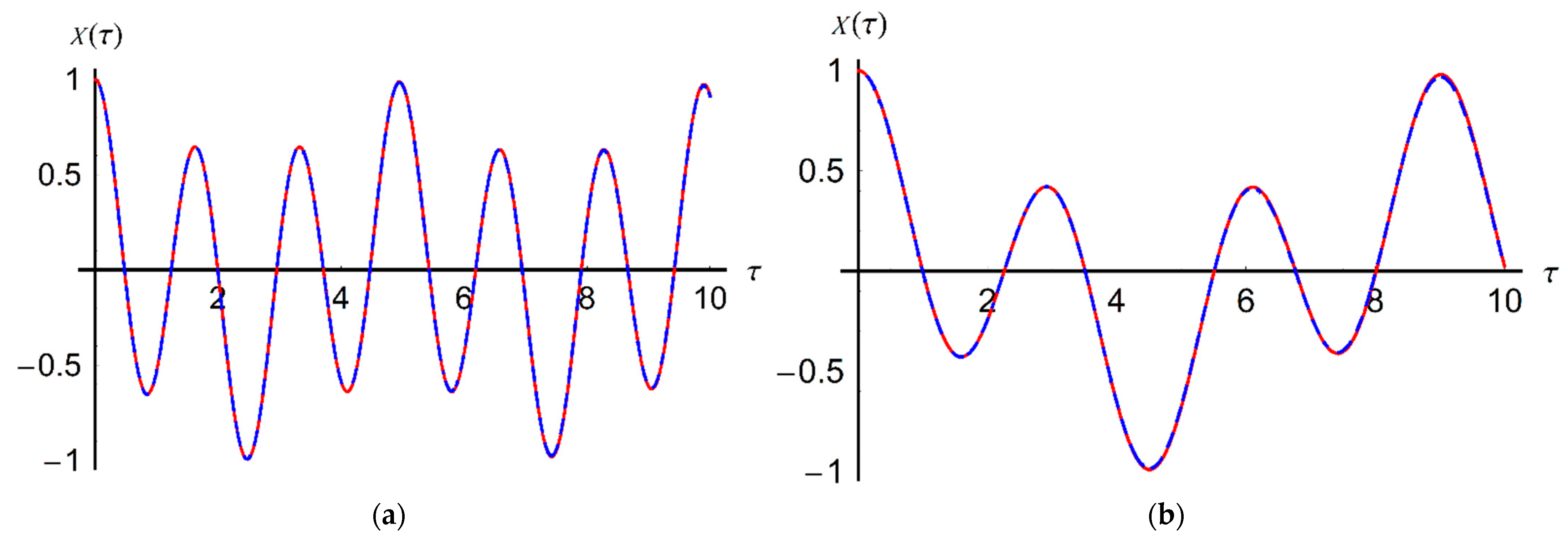
Now, to prove the accuracy and the effectiveness of our method, we consider a set of numerical values for the physical parameters involved in the governing equations; i.e., M₁ = 0.072, M₂ = 0.086, K₁ = 110, K₂ = 141, a = 3.

Figure 2 presents a comparison between the approximate solution (35) and corresponding numerical integration results obtained by means of a fourth-order Runge–Kutta method.

This comparison emphasizes the high accuracy of the proposed analytical solution obtained through OAFM. Figure 3 presents the corresponding phase portraits.

5. Analysis of Non-Periodic Motion

In this section, we present some possible situations, depending on the motions of the masses M₁ and M₂ of the dynamical system considered in Section 2. Depending on the perturbing force F and initial conditions, we present the following possible cases of non-periodic motions.

Case 5.1. The oscillator of mass M₁ is moving from the static equilibrium position to the position of the impact with the wall W₁. If the moment of impact M₁ with W_1is τ₁, then this case takes place if $X(\mathsf{\tau })\le 1$, X(τ₁) = 0 and $\dot{X}({\mathsf{\tau }}_1)\le 0$. In particular, if $\dot{X}({\mathsf{\tau }}_1)=0$, then the oscillator M₁ stops at the wall W₁. The velocity of the mass M₁ after the impact will be $\dot{X}({\mathsf{\tau }}_1^{+})=-R_2\dot{X}({\mathsf{\tau }}_1^{-})$, where the symbols “+” and “−” indicate the moments after and before the impact, respectively, and R₂ is the coefficient of restitution. For the oscillator of mass M₂, the following situations are possible (types of movement):

(a)

The oscillator M₂ is moving between the oscillator of mass M₁ and the wall W₂ without impact and without sticking motion. The condition is equivalent to the existence of the inequalities $X(\mathsf{\tau })<Y(\mathsf{\tau })<1+{\mathsf{\delta }}_2/{\mathsf{\delta }}_1+{\mathsf{\delta }}_3/{\mathsf{\delta }}_1$ and τ < τ_1. It follows that there exists a moment of time ${\mathsf{\tau }}_1^{*}$ when M₂ stops, $\dot{Y}({\mathsf{\tau }}_1^{*})=0$.

(b)

The oscillator M₂ impacts the oscillator M₁ before the collision of the mass M₁ with the wall W₁. In this case, there exists a moment τ₂ < τ so that X(τ₂) = Y(τ₂), $\dot{X}({\mathsf{\tau }}_2)<0,\dot{Y}({\mathsf{\tau }}_2)<0$, and $\dot{X}({\mathsf{\tau }}_2)\ne \dot{Y}({\mathsf{\tau }}_2)$. After this collision, the velocities can be written as:

$$\begin{array}{l}\dot{X}({\mathsf{\tau }}_2^{+})=\frac{M_1-R{M}_2}{M_1+M_2}\dot{X}({\mathsf{\tau }}_2^{-})+\frac{M_2(1+R)}{M_1+M_2}\dot{Y}({\mathsf{\tau }}_2^{-}),\\ \dot{Y}({\mathsf{\tau }}_2^{+})=\frac{M_1(1+R)}{M_1+M_2}\dot{X}({\mathsf{\tau }}_2^{-})+\frac{M_2-R{M}_1}{M_1+M_2}\dot{Y}({\mathsf{\tau }}_2^{-})\begin{array}{cc};& \dot{X}({\mathsf{\tau }}_2^{-})=\dot{X}({\mathsf{\tau }}_2)\end{array}\begin{array}{cc};& \dot{Y}({\mathsf{\tau }}_2^{+})=\dot{Y}({\mathsf{\tau }}_2^{})\end{array},\end{array}$$

(37)

(c)

The oscillator of mass M₁ is sticking to M₂ (sticking motion). The condition is written as X(τ₂) = Y(τ₂) and $\dot{X}({\mathsf{\tau }}_2)=\dot{Y}({\mathsf{\tau }}_2)$. The contact force corresponding to masses M₁ and M₂ is obtained from Equations (4) and (5):

$$\begin{array}{l}{F}_{12}(\mathsf{\tau })=2a\mathsf{\Omega }(k{\mathsf{\alpha }}_2-\mathsf{\Omega }{\mathsf{\alpha }}_1)\sin \mathsf{\Omega }\mathsf{\tau }+(a-a{k}^2+3a\mathsf{\beta }{X}_{}^2+\frac{3}{4}\mathsf{\beta }{a}^3)\cos \mathsf{\Omega }\mathsf{\tau }-\frac{3}{2}{a}^2\mathsf{\beta }X\cos 2\mathsf{\Omega }\mathsf{\tau }+\frac{\mathsf{\beta }}{4}{a}^3\cos 3\mathsf{\Omega }\mathsf{\tau }+2{\mathsf{\alpha }}_2\dot{Y}-\\ -2{\mathsf{\alpha }}_1\dot{X}+k^{2}Y-(1+\frac{3}{2}{a}^2)X-\mathsf{\beta }{X}^3.\end{array}$$

(38)

The sticking takes place only if F₁₂ > 0.

(d)

The oscillator of mass M₂ impacts the wall W₂ at the moment τ = τ₃. The conditions are $Y({\mathsf{\tau }}_3)=1+{\mathsf{\delta }}_2/{\mathsf{\delta }}_1+{\mathsf{\delta }}_3/{\mathsf{\delta }}_1$ and $\dot{Y}({\mathsf{\tau }}_3)\ge 0$. If $\dot{Y}({\mathsf{\tau }}_3)=0$, then the oscillator M₂ stops without impacting the wall W₂.

Case 5.2. The oscillator of mass M₁ is moving without impact from the position of static equilibrium between the wall W₁ and the oscillator of mass M₂. The oscillator of mass M₁ stops at the moment $\mathsf{\tau }={{\mathsf{\tau }}^{\prime }}_1$ before reaching the wall W₁, then stops at the moment $\mathsf{\tau }={{\mathsf{\tau }}^{″}}_1$, before reaching the oscillator of mass M₂, so that $\dot{X}({{\mathsf{\tau }}^{\prime }}_1)=\dot{X}({{\mathsf{\tau }}^{″}}_1)=0$. For the oscillator of mass M₂, one can identify two situations:

(a)

The oscillator of mass M₂ is moving without impact between the oscillator of mass M₁ and the wall W₂, so that one can write $X(\mathsf{\tau })<Y(\mathsf{\tau })<1+{\mathsf{\delta }}_2/{\mathsf{\delta }}_1+{\mathsf{\delta }}_3/{\mathsf{\delta }}_1$. It results that there exist two moments: ${{\mathsf{\tau }}^{\prime }}_2$, when the oscillator of mass M₂ stops before the oscillator M₂; and ${{\mathsf{\tau }}^{″}}_2$, when the oscillator M₂ stops before the wall W₂, so that $\dot{Y}({{\mathsf{\tau }}^{\prime }}_2)=\dot{Y}({{\mathsf{\tau }}^{″}}_2)=0$.

(b)

The oscillator of mass M₂ moving between the oscillator of mass M₁ without impact and the wall W₂ with impact, so that $X(\mathsf{\tau })<Y(\mathsf{\tau })\le 1+{\mathsf{\delta }}_2/{\mathsf{\delta }}_1+{\mathsf{\delta }}_3/{\mathsf{\delta }}_1$. The moment of impact of the oscillator M₂ with the wall W₂ is τ₄. It follows the condition $Y({\mathsf{\tau }}_4)=1+{\mathsf{\delta }}_2/{\mathsf{\delta }}_1+{\mathsf{\delta }}_3/{\mathsf{\delta }}_1$ and $\dot{Y}({\mathsf{\tau }}_4^{-})>0$. After the impact, the following expression takes place: $\dot{Y}({\mathsf{\tau }}_4^{+})=-R\dot{Y}({\mathsf{\tau }}_4^{-})$.

Case 5.3. In this last case, the oscillator of mass M₁ is moving from the static equilibrium position toward the oscillator of mas M₂, $X(\mathsf{\tau })\ge 1$. For the oscillator of mass M₂, the following five situations are possible:

(a)

The oscillator of mass M₂ is moving from the position of static equilibrium $Y(0)=1+{\mathsf{\delta }}_2/{\mathsf{\delta }}_1$ toward the oscillator of mass M₁ without impact. The conditions are $X(\mathsf{\tau })<Y(\mathsf{\tau })$, $Y(\mathsf{\tau })<1+{\mathsf{\delta }}_2/{\mathsf{\delta }}_1$, and $\dot{Y}(0)\le 0$. In this subcase, there exists a moment τ₅ so that $\dot{Y}({\mathsf{\tau }}_5)=0$.

(b)

The oscillator of mass M₂ is moving from the position of static equilibrium toward the oscillator of mass M₁ with impact. The corresponding conditions for this subcase are $X(\mathsf{\tau })\le Y(\mathsf{\tau })<1+{\mathsf{\delta }}_2/{\mathsf{\delta }}_1$, and there exists a moment τ₆ when X(τ₆) = Y(τ₆) and $\dot{Y}({\mathsf{\tau }}_6)<0$. After the impact, the velocities of the oscillators will be:

$$\begin{array}{l}\dot{X}({\mathsf{\tau }}_6^{+})=\frac{M_1-R{M}_2}{M_1+M_2}\dot{X}({\mathsf{\tau }}_6^{})+\frac{M_2(1+R)}{M_1+M_2}\dot{Y}({\mathsf{\tau }}_6^{}),\\ \dot{Y}({\mathsf{\tau }}_6^{+})=\frac{M_1(1+R)}{M_1+M_2}\dot{X}({\mathsf{\tau }}_6^{})+\frac{M_2-R{M}_1}{M_1+M_2}\dot{Y}({\mathsf{\tau }}_6^{}).\end{array}$$

(39)

(c)

The oscillator of mass M₂ is moving from the position of static equilibrium toward the wall W₂ without impact with the oscillator of mass M₁ or with the wall W₂. This subcase takes place if $X(\mathsf{\tau })\ge 1$, $Y(\mathsf{\tau })\ge 1+{\mathsf{\delta }}_2/{\mathsf{\delta }}_1$, and X(τ) < Y(τ). It is clear that there exist two moments ${{\mathsf{\tau }}^{\prime }}_7$ and ${{\mathsf{\tau }}^{″}}_7$ when $\dot{X}({{\mathsf{\tau }}^{\prime }}_7)=0$, which means the oscillator of mass M₁ stops; and $\dot{Y}({{\mathsf{\tau }}^{″}}_7)=0$, which means the oscillator of mass M₂ stops.

(d)

The oscillator of mass M₂ is moving from the position of static equilibrium toward the wall W₂, but with impact between the two oscillators. The impact takes place before the oscillator of mass M₂ to reach at the wall W₂ and without sticking. The conditions will be $X(\mathsf{\tau })\ge 1,Y(\mathsf{\tau })\ge 1+{\mathsf{\delta }}_2/{\mathsf{\delta }}_1$, and there exists a moment τ₇ when $X({\mathsf{\tau }}_7)=Y({\mathsf{\tau }}_7)$, $\dot{X}({{\mathsf{\tau }}^{\prime }}_7)>0$, $\dot{Y}({\mathsf{\tau }}_7)\ge 0$, and $\dot{X}({\mathsf{\tau }}_7)>\dot{Y}({\mathsf{\tau }}_7)$. If the impact of the oscillators takes place with sticking, then the condition is similar to (38), $F_{12}(\mathsf{\tau })>0,\mathsf{\tau }>{\mathsf{\tau }}_7$.

(e)

The oscillator of mass M₂ is moving toward the wall W₂, and the impact with W₂ takes place at the moment τ₈, but there is no impact between the two oscillators. Therefore, the following conditions should be satisfied:

$$X(\mathsf{\tau })<Y(\mathsf{\tau })\le 1+\frac{{\mathsf{\delta }}_2}{{\mathsf{\delta }}_1}+\frac{{\mathsf{\delta }}_3}{{\mathsf{\delta }}_1}\begin{array}{cc};& Y(\end{array}{\mathsf{\tau }}_8)=1+\frac{{\mathsf{\delta }}_2}{{\mathsf{\delta }}_1}+\frac{{\mathsf{\delta }}_3}{{\mathsf{\delta }}_1}\begin{array}{cc};& \dot{Y}\end{array}({\mathsf{\tau }}_8)>0.$$

(40)

After the impact, the velocity of the oscillator of mass M₂ is $\dot{Y}({\mathsf{\tau }}_8^{+})=-R\dot{Y}({\mathsf{\tau }}_8^{-})$.

It should be stated that after the two oscillators undergo one of the movements studied before, the movement of each oscillator should be studied by taking into account the conditions mentioned for the corresponding case. For example, after Case 5.1a takes place, therefore in the condition $\dot{X}({\mathsf{\tau }}_1)<0$ (the oscillator of mass M₁ does not stop), $\dot{X}({\mathsf{\tau }}_1^{+})=-R\dot{X}({\mathsf{\tau }}_1^{-})$, and $\dot{Y}({\mathsf{\tau }}_1^{*})=0$, then the approximate solutions (35) and (36) will be written as:

$$\begin{array}{l}\overline{X}(\mathsf{\tau })=e^{-{\mathsf{\alpha }}_1(\mathsf{\tau }-{\mathsf{\tau }}_1)}\frac{R_2\dot{X}({\mathsf{\tau }}_1^{-})}{\sqrt{{\overline{\mathsf{\Omega }}}^2-{\mathsf{\alpha }}_1^2}}\sin \sqrt{{\overline{\mathsf{\Omega }}}^2-{\mathsf{\alpha }}_1^2}(\mathsf{\tau }-{\mathsf{\tau }}_1)+\frac{9a}{8+12a^2}[\cos \mathsf{\Omega }(\mathsf{\tau }-{\mathsf{\tau }}_1)-\cos 3\mathsf{\Omega }(\mathsf{\tau }-{\mathsf{\tau }}_1)]+\\ +\frac{(36a^3-3a)\mathsf{\Omega }{\mathsf{\alpha }}_1}{8{(2+3a^2)}^2}[\sin 3\mathsf{\Omega }(\mathsf{\tau }-{\mathsf{\tau }}_1)-3\sin \mathsf{\Omega }(\mathsf{\tau }-{\mathsf{\tau }}_1)]\begin{array}{cc},& \mathsf{\tau }\ge {\mathsf{\tau }}_1\end{array},\end{array}$$

(41)

$$\begin{array}{l}Y(\mathsf{\tau })=e^{-{\mathsf{\alpha }}_{2}k(\mathsf{\tau }-{\mathsf{\tau }}_1^{*})}\left[(\gamma -Q_3)\cos \sqrt{k^2-k{\mathsf{\alpha }}_2}(\mathsf{\tau }-{\mathsf{\tau }}_1^{*})+\frac{{\mathsf{\alpha }}_{2}k(\gamma -Q_3)-\mathsf{\Omega }{Q}_4}{\sqrt{k^2-k{\mathsf{\alpha }}_2}}\sin \sqrt{k^2-k{\mathsf{\alpha }}_2}(\mathsf{\tau }-{\mathsf{\tau }}_1^{*})\right]+\\ +Q_3\cos \mathsf{\Omega }(\mathsf{\tau }-{\mathsf{\tau }}_1^{*})+Q_4\sin \mathsf{\Omega }(\mathsf{\tau }-{\mathsf{\tau }}_1^{*}),\end{array}$$

(42)

where ${\mathsf{\tau }}_1^{*}$ is obtained from the equation $\dot{Y}({\mathsf{\tau }}_1^{*})=0$; $\gamma =Y({\mathsf{\tau }}_1^{*})$, $Y({\mathsf{\tau }}_1^{*})$ is given by Equation (36); and Q₃ and Q₄ are given by Equation (34).

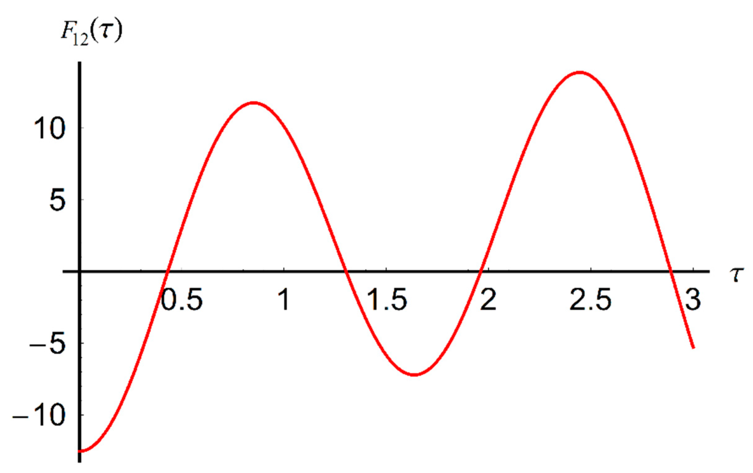
Figure 4 shows the contact force of (38).

It can be seen that the contact force has two maximum points at τ = 0.8 and τ = 2.4, and is null for four points: τ = 0.4, τ = 1.3, τ = 1.9, and τ = 2.9.

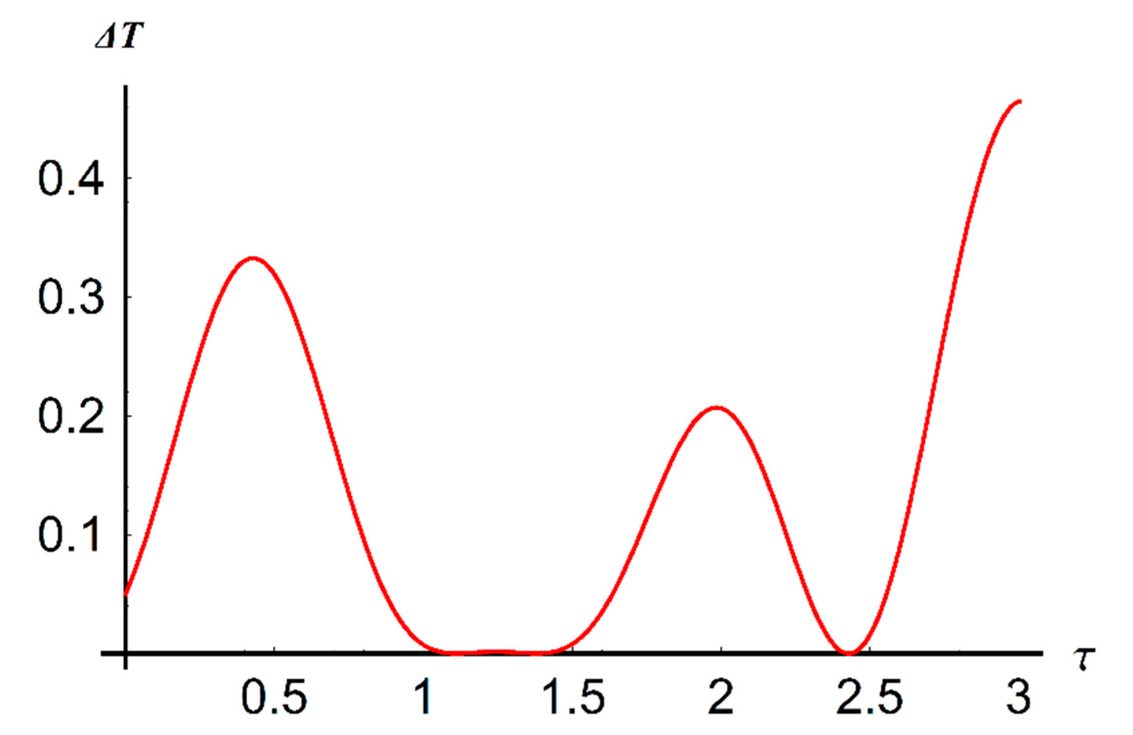
Another specific element for the impact phenomenon is the kinetic energy loss. At the moment of impact, the kinetic energy is transformed into work, caloric energy, etc. The kinetic energy loss is given by the difference between the kinetic energy at the beginning and at the end of impact:

$$\Delta T=\frac{1}{2}{M}_1{\dot{X}}^2({\mathsf{\tau }}^{-})+\frac{1}{2}{M}_2{\dot{Y}}^2({\mathsf{\tau }}^{-})-\frac{1}{2}{M}_1{\dot{X}}^2({\mathsf{\tau }}^{+})-\frac{1}{2}{M}_2{\dot{Y}}^2({\mathsf{\tau }}^{+}).$$

(43)

In Case 5.1b, the kinetic energy loss becomes:

$$\Delta T=\frac{M_1{M}_2}{2(M_1+M_2)}{\left[\dot{X}(\mathsf{\tau })-\dot{Y}(\mathsf{\tau })\right]}^2(1-R^2).$$

(44)

Figure 5 presents the kinetic energy loss for Case 5.1b.

6. Analysis of Periodic Motion

The solutions (35) and (36) are written for the initial conditions in (6), in the absence of impact. After some time, the free vibration described by (35) and (36) disappear, so that the movement becomes periodic with the same period of the perturbing force F, which is $T=2\mathsf{\pi }/\mathsf{\Omega }$.

The problem of the stability of periodic motion is of interest only in the case of the impact between the two oscillators, since the impact with the walls W₁ and W₂ is assumed to be elastic. In the general case, instead of the conditions in (6), we consider that the approximate solution $\overline{X}(\mathsf{\tau })$ and the exact solution Y(τ) are:

$$\begin{array}{l}\overline{X}(\mathsf{\tau })=e^{-{\mathsf{\alpha }}_1\mathsf{\tau }}\left(C_1\cos \sqrt{{\overline{\mathsf{\Omega }}}^2-{\mathsf{\alpha }}_1^2}\mathsf{\tau }+C_2\sin \sqrt{{\overline{\mathsf{\Omega }}}^2-{\mathsf{\alpha }}_1^2}\mathsf{\tau }\right)+\frac{9a^2}{8+12a^2}[\cos (\mathsf{\Omega }\mathsf{\tau }+\varphi )-\cos (3\mathsf{\Omega }\mathsf{\tau }+3\varphi )]+\\ +\frac{(36a^3-3a)\mathsf{\Omega }{\mathsf{\alpha }}_1}{8{(2+3a^2)}^2}[\sin (3\mathsf{\Omega }\mathsf{\tau }+3\varphi )-\sin (\mathsf{\Omega }\mathsf{\tau }+\varphi )],\end{array}$$

(45)

$$Y(\mathsf{\tau })=e^{-{\mathsf{\alpha }}_{2}k\mathsf{\tau }}\left[C_3\cos \sqrt{k^2-k{\mathsf{\alpha }}_2}\mathsf{\tau }+C_4\sin \sqrt{k^2-k{\mathsf{\alpha }}_2}\mathsf{\tau }\right]+Q_3\cos (\mathsf{\Omega }\mathsf{\tau }+\varphi )+Q_4\sin (\mathsf{\Omega }\mathsf{\tau }+\varphi ).$$

(46)

where Q₃ and Q₄ are given by Equation (34), and C₁–C₄ and ϕ are determined from initial conditions.

Solutions (45) and (46) are stable if a negligible change of a small perturbation takes place in the initial conditions and delay at any time interval. If the change is significant, then the solutions become unstable.

In this section, we consider small perturbations for τ, C₁–C₄, and delay ϕ: ∆τ, ∆C₁,…, ∆C₄, ∆ϕ, so that ([4,5,6,7,32]):

$$\begin{array}{l}\overline{X}(\mathsf{\tau }+\Delta \mathsf{\tau })=e^{-{\mathsf{\alpha }}_1(\mathsf{\tau }+\Delta \mathsf{\tau })}\left[(C_1+\Delta C_1)\cos \sqrt{{\overline{\mathsf{\Omega }}}^2-{\mathsf{\alpha }}_1^2}(\mathsf{\tau }+\Delta \mathsf{\tau })+(C_2+\Delta C_2)\sin \sqrt{{\overline{\mathsf{\Omega }}}^2-{\mathsf{\alpha }}_1^2}(\mathsf{\tau }+\Delta \mathsf{\tau })\right]+\\ +\frac{9a^2}{8+12a^2}[\cos (\mathsf{\Omega }\mathsf{\tau }+\mathsf{\Omega }\Delta \mathsf{\tau }+\varphi +\Delta \varphi )-\cos (3\mathsf{\Omega }\mathsf{\tau }+3\mathsf{\Omega }\Delta \mathsf{\tau }+3\varphi +3\Delta \varphi )]+\\ +\frac{(36a^3-3a)\mathsf{\Omega }{\mathsf{\alpha }}_1}{8{(2+3a^2)}^2}[\sin (3\mathsf{\Omega }\mathsf{\tau }+3\mathsf{\Omega }\Delta \mathsf{\tau }+3\varphi +3\Delta \varphi )-\sin (\mathsf{\Omega }\mathsf{\tau }+\mathsf{\Omega }\Delta \mathsf{\tau }+\varphi +\Delta \varphi )],\end{array}$$

(47)

$$\begin{array}{l}Y(\mathsf{\tau }+\Delta \mathsf{\tau })=e^{-{\mathsf{\alpha }}_{2}k(\mathsf{\tau }+\Delta \mathsf{\tau })}\left[(C_3+\Delta C_3)\cos \sqrt{k^2-k{\mathsf{\alpha }}_2}(\mathsf{\tau }+\Delta \mathsf{\tau })+(C_4+\Delta C_4)\sin \sqrt{k^2-k{\mathsf{\alpha }}_2}(\mathsf{\tau }+\Delta \mathsf{\tau })\right]+\\ +Q_3\cos (\mathsf{\Omega }\mathsf{\tau }+\mathsf{\Omega }\Delta \mathsf{\tau }+\varphi +\Delta \varphi )+Q_4\sin (\mathsf{\Omega }\mathsf{\tau }+\mathsf{\Omega }\Delta \mathsf{\tau }+\varphi +\Delta \varphi ),\end{array}$$

(48)

Taking into account the approximations:

$$e^{-\mathsf{\alpha }\Delta \mathsf{\tau }}\approx 1-\mathsf{\alpha }\Delta \mathsf{\tau }\begin{array}{cc};& \cos (\mathsf{\alpha }\mathsf{\tau }+\Delta \mathsf{\tau })=\end{array}\cos \mathsf{\alpha }\mathsf{\tau }-\Delta \mathsf{\tau }\sin \mathsf{\alpha }\mathsf{\tau }\begin{array}{cc};& \sin \end{array}(\mathsf{\alpha }\mathsf{\tau }+\Delta \mathsf{\tau })=\sin \mathsf{\alpha }\mathsf{\tau }+\Delta \mathsf{\tau }\cos \mathsf{\alpha }\mathsf{\tau },$$

(49)

and the modifications of the solutions $\overline{X}$ and Y:

$$\Delta \overline{X}(\mathsf{\tau })=\overline{X}(\mathsf{\tau }+\Delta \mathsf{\tau })-\overline{X}(\mathsf{\tau })\begin{array}{cc};& \Delta Y(\mathsf{\tau })=Y(\mathsf{\tau }+\Delta \mathsf{\tau })-Y(\mathsf{\tau })\end{array},$$

(50)

after linearization of Equations (47) and (48) can be written as:

$$\begin{array}{l}\Delta \overline{X}(\mathsf{\tau })=e^{-{\mathsf{\alpha }}_1\mathsf{\tau }}[-\Delta \mathsf{\tau }(\mathsf{\alpha }1C_1\cos \sqrt{{\overline{\mathsf{\Omega }}}^2-{\mathsf{\alpha }}_1^2}\mathsf{\tau }+C_1\sqrt{{\overline{\mathsf{\Omega }}}^2-{\mathsf{\alpha }}_1^2}\sin \sqrt{{\overline{\mathsf{\Omega }}}^2-{\mathsf{\alpha }}_1^2}\mathsf{\tau }+{\mathsf{\alpha }}_1{C}_2\sin \sqrt{{\overline{\mathsf{\Omega }}}^2-{\mathsf{\alpha }}_1^2}\mathsf{\tau }-\\ -C_2\sqrt{{\overline{\mathsf{\Omega }}}^2-{\mathsf{\alpha }}_1^2}\cos \sqrt{{\overline{\mathsf{\Omega }}}^2-{\mathsf{\alpha }}_1^2}\mathsf{\tau })+\Delta C_1\cos \sqrt{{\overline{\mathsf{\Omega }}}^2-{\mathsf{\alpha }}_1^2}\mathsf{\tau }+\Delta C{}_2\sin \sqrt{{\overline{\mathsf{\Omega }}}^2-{\mathsf{\alpha }}_1^2}\mathsf{\tau }]+\frac{9a^2}{8+12a^2}[(\mathsf{\Omega }\Delta \mathsf{\tau }+\Delta \varphi )(3\sin (3\mathsf{\Omega }\mathsf{\tau }+3\varphi )-\\ -\sin (\mathsf{\Omega }\mathsf{\tau }+\varphi )]+\frac{(108a^3-9a)\mathsf{\Omega }{\mathsf{\alpha }}_1}{8{(2+3a^2)}^2}(\mathsf{\Omega }\Delta \mathsf{\tau }+\Delta \varphi )[3\cos (3\mathsf{\Omega }\mathsf{\tau }+3\varphi )-\cos (\mathsf{\Omega }\mathsf{\tau }+\varphi )],\end{array}$$

(51)

$$\begin{array}{l}\Delta Y(\mathsf{\tau })=e^{-{\mathsf{\alpha }}_{2}k\mathsf{\tau }}[-\Delta \mathsf{\tau }({\mathsf{\alpha }}_{2}k{C}_3\cos \sqrt{k^2-k{\mathsf{\alpha }}_2}\mathsf{\tau }+C_3\sqrt{k^2-k{\mathsf{\alpha }}_2}\sin \sqrt{k^2-k{\mathsf{\alpha }}_2}\mathsf{\tau }-C_4\sqrt{k^2-k{\mathsf{\alpha }}_2}\cos \sqrt{k^2-k{\mathsf{\alpha }}_2}\mathsf{\tau }+\\ +{\mathsf{\alpha }}_{2}k{C}_4\sin \sqrt{k^2-k{\mathsf{\alpha }}_2}\mathsf{\tau })+\Delta C_3\cos \sqrt{k^2-k{\mathsf{\alpha }}_2}\mathsf{\tau }+\Delta C_4\sin \sqrt{k^2-k{\mathsf{\alpha }}_2}\mathsf{\tau }]+\\ +Q_4(\mathsf{\Omega }\Delta \mathsf{\tau }+\Delta \varphi )\cos (\mathsf{\Omega }\mathsf{\tau }+\varphi )-Q_3(\mathsf{\Omega }\Delta \mathsf{\tau }+\Delta \varphi )\sin (\mathsf{\Omega }\mathsf{\tau }+\varphi ),\end{array}$$

(52)

After differentiating Equations (51) and (52), one obtains:

$$\begin{array}{l}\Delta \dot{\overline{X}}(\mathsf{\tau })=e^{-{\mathsf{\alpha }}_1\mathsf{\tau }}[\Delta \mathsf{\tau }({\overline{\mathsf{\Omega }}}^2{C}_1\cos \sqrt{{\overline{\mathsf{\Omega }}}^2-{\mathsf{\alpha }}_1^2}\mathsf{\tau }+2{\mathsf{\alpha }}_1{C}_1\sqrt{{\overline{\mathsf{\Omega }}}^2-{\mathsf{\alpha }}_1^2}\sin \sqrt{{\overline{\mathsf{\Omega }}}^2-{\mathsf{\alpha }}_1^2}\mathsf{\tau }+{\overline{\mathsf{\Omega }}}^2{C}_2\sin \sqrt{{\overline{\mathsf{\Omega }}}^2-{\mathsf{\alpha }}_1^2}\mathsf{\tau }-\\ -2{\mathsf{\alpha }}_1{C}_2\cos \sqrt{{\overline{\mathsf{\Omega }}}^2-{\mathsf{\alpha }}_1^2}\mathsf{\tau })-\Delta C_1({\mathsf{\alpha }}_1\cos \sqrt{{\overline{\mathsf{\Omega }}}^2-{\mathsf{\alpha }}_1^2}\mathsf{\tau }+\sqrt{{\overline{\mathsf{\Omega }}}^2-{\mathsf{\alpha }}_1^2}\sin \sqrt{{\overline{\mathsf{\Omega }}}^2-{\mathsf{\alpha }}_1^2}\mathsf{\tau })+\\ +\Delta C_2(\sqrt{{\overline{\mathsf{\Omega }}}^2-{\mathsf{\alpha }}_1^2}\cos \sqrt{{\overline{\mathsf{\Omega }}}^2-{\mathsf{\alpha }}_1^2}\mathsf{\tau }-{\mathsf{\alpha }}_1\sin \sqrt{{\overline{\mathsf{\Omega }}}^2-{\mathsf{\alpha }}_1^2}\mathsf{\tau }]+\frac{9a\mathsf{\Omega }}{8+12a^2}(\mathsf{\Omega }\Delta \mathsf{\tau }+\Delta \varphi )[(9\cos (3\mathsf{\Omega }\mathsf{\tau }+3\varphi )-\cos (\mathsf{\Omega }\mathsf{\tau }+\varphi )]+\\ +\frac{(108a^3-9a){\mathsf{\Omega }}^2{\mathsf{\alpha }}_1}{8{(2+3a^2)}^2}(\mathsf{\Omega }\Delta \mathsf{\tau }+\Delta \varphi )[\sin (\mathsf{\Omega }\mathsf{\tau }+\varphi )-9\sin (3\mathsf{\Omega }\mathsf{\tau }+3\varphi )],\end{array}$$

(53)

$$\begin{array}{l}\Delta \dot{Y}(\mathsf{\tau })=e^{-{\mathsf{\alpha }}_{2}k\mathsf{\tau }}[\Delta \mathsf{\tau }(k^2{C}_3\cos \sqrt{k^2-k{\mathsf{\alpha }}_2}\mathsf{\tau }+2{\mathsf{\alpha }}_{2}k{C}_3\sqrt{k^2-k{\mathsf{\alpha }}_2}\sin \sqrt{k^2-k{\mathsf{\alpha }}_2}\mathsf{\tau }+k^2{C}_4\sin \sqrt{k^2-k{\mathsf{\alpha }}_2}\mathsf{\tau }-\\ -2{\mathsf{\alpha }}_{2}k{C}_3\cos \sqrt{k^2-k{\mathsf{\alpha }}_2}\mathsf{\tau })-\Delta C_3({\mathsf{\alpha }}_{2}k\cos \sqrt{k^2-k{\mathsf{\alpha }}_2}\mathsf{\tau }+\sqrt{k^2-k{\mathsf{\alpha }}_2}\sin \sqrt{k^2-k{\mathsf{\alpha }}_2}\mathsf{\tau })+\Delta C_4(\sqrt{k^2-k{\mathsf{\alpha }}_2}\cos \sqrt{k^2-k{\mathsf{\alpha }}_2}\mathsf{\tau }-\\ -{\mathsf{\alpha }}_{2}k\sin \sqrt{k^2-k{\mathsf{\alpha }}_2}\mathsf{\tau }]-\mathsf{\Omega }{Q}_3(\mathsf{\Omega }\Delta \mathsf{\tau }+\Delta \varphi )\cos (\mathsf{\Omega }\mathsf{\tau }+\varphi )-\mathsf{\Omega }{Q}_4(\mathsf{\Omega }\Delta \mathsf{\tau }+\Delta \varphi )\sin (\mathsf{\Omega }\mathsf{\tau }+\varphi ).\end{array}$$

(54)

For the perturbed motion described by Equations (51) and (52), the initial conditions at two moments—after the n-th impact and before the (n + 1)-th impact—are written as:

$$n:\begin{array}{cc}& \mathsf{\tau }=0\begin{array}{cc},& \Delta {\mathsf{\tau }}_n=0\begin{array}{cc},& \Delta {\overline{X}}_n=\Delta Y_n=0\end{array}\end{array}\end{array}\begin{array}{cc},& \Delta {\dot{\overline{X}}}_n=\Delta {\dot{\overline{X}}}_n^{+}\end{array}\begin{array}{cc},& \Delta {\dot{Y}}_n=\Delta {\dot{Y}}_n^{+}\end{array},$$

(55)

$$n+1:\begin{array}{cc}& \mathsf{\tau }=\frac{2n\mathsf{\pi }}{\mathsf{\Omega }}+\Delta {\mathsf{\tau }}_n\begin{array}{cc},& \Delta {\mathsf{\tau }}_n=\Delta T_n=\frac{\Delta {\varphi }_{n+1}-\Delta {\varphi }_n}{\mathsf{\Omega }}\begin{array}{cc},& \Delta {\overline{X}}_n=\Delta Y_n=0\end{array}\end{array}\end{array}\begin{array}{cc},& \Delta {\dot{\overline{X}}}_n=\Delta {\dot{\overline{X}}}_n^{-}\end{array}\begin{array}{cc},& \Delta {\dot{Y}}_n=\Delta {\dot{Y}}_n^{-}\end{array},$$

(56)

where

$$\Delta {\overline{X}}_n=\Delta \overline{X}\left(\frac{2n\mathsf{\pi }}{\mathsf{\Omega }}+\Delta \mathsf{\tau }\right)\begin{array}{cc},& \Delta Y_n=\Delta Y\left(\frac{2n\mathsf{\pi }}{\mathsf{\Omega }}+\Delta {\mathsf{\tau }}^{*}\right)\end{array}.$$

(57)

Then, the velocities after the impact become:

$$\begin{array}{l}\Delta {\dot{\overline{X}}}_n^{+}(0)=\frac{M_1-R{M}_2}{M_1+M_2}\Delta {\dot{\overline{X}}}_n^{-}\left(\frac{2n\mathsf{\pi }}{\mathsf{\Omega }}+\Delta T_n\right)+\frac{M_2(1+R)}{M_1+M_2}\Delta {\dot{Y}}_n^{-}\left(\frac{2n\mathsf{\pi }}{\mathsf{\Omega }}+\Delta T_n^{*}\right),\\ \Delta {\dot{Y}}_n^{+}(0)=\frac{M_1(1+R)}{M_1+M_2}\Delta {\dot{\overline{X}}}_n^{-}\left(\frac{2n\mathsf{\pi }}{\mathsf{\Omega }}+\Delta T_n\right)+\frac{M_2-R{M}_1}{M_1+M_2}\Delta {\dot{Y}}_n^{-}\left(\frac{2n\mathsf{\pi }}{\mathsf{\Omega }}+\Delta T_n^{*}\right).\end{array}$$

(58)

From Equations (51)–(53), one obtains:

$$\Delta {\overline{X}}_n(0)=\Delta C_{1n}+\left[\frac{9a(3\sin 3\varphi -\sin \varphi )}{8+12a^2}+\frac{(108a^3-9a)\mathsf{\Omega }{\mathsf{\alpha }}_1(3\cos 3\varphi -\cos \varphi )}{8{(2+3a^2)}^2}\right]\Delta {\varphi }_n,$$

(59)

$$\Delta Y_n(0)=\Delta C_{3n}+(Q_4\cos \varphi -Q_3\sin \varphi )\Delta {\varphi }_n^{*}.$$

(60)

From Equations (53)–(55), one obtains:

$$\Delta {\dot{\overline{X}}}_n^{+}(0)=-{\mathsf{\alpha }}_1\Delta C_{1n}+\sqrt{{\overline{\mathsf{\Omega }}}^2-{\mathsf{\alpha }}_1^2}\Delta C_{2n}+\left[\frac{9a\mathsf{\Omega }(9\cos 3\varphi -\cos \varphi )}{8+12a^2}+\frac{(108a^3-9a){\mathsf{\Omega }}^2{\mathsf{\alpha }}_1(\sin \varphi -9\sin 3\varphi )}{8{(2+3a^2)}^2}\right]\Delta {\varphi }_n,$$

(61)

$$\Delta {\dot{Y}}_n^{+}(0)=-{\mathsf{\alpha }}_{2}k\Delta C_{3n}+\sqrt{k^2-k{\mathsf{\alpha }}_2}\Delta C_{4n}-(\mathsf{\Omega }{Q}_3\cos \varphi +\mathsf{\Omega }{Q}_4\sin \varphi )\Delta {\varphi }_n^{*}.$$

(62)

Analogously, from Equations (51), (52), and (56), one obtains:

$$\begin{array}{l}\Delta {\overline{X}}_n(\frac{2n\mathsf{\pi }}{\mathsf{\Omega }}+\Delta {\mathsf{\tau }}_n)=e^{-\frac{2n\mathsf{\pi }{\mathsf{\alpha }}_1}{\mathsf{\Omega }}}\{-[\left({\mathsf{\alpha }}_1{C}_1-C_2\sqrt{{\overline{\mathsf{\Omega }}}^2-{\mathsf{\alpha }}_1^2}\right)\cos \frac{2n\mathsf{\pi }\sqrt{{\overline{\mathsf{\Omega }}}^2-{\mathsf{\alpha }}_1^2}}{\mathsf{\Omega }}+(C_1\sqrt{{\overline{\mathsf{\Omega }}}^2-{\mathsf{\alpha }}_1^2}+\\ +{\mathsf{\alpha }}_1{C}_2)\sin \frac{2n\mathsf{\pi }\sqrt{{\overline{\mathsf{\Omega }}}^2-{\mathsf{\alpha }}_1^2}}{\mathsf{\Omega }}]\frac{\Delta {\varphi }_{n+1}-\Delta {\varphi }_n}{\mathsf{\Omega }}+\Delta C_1\cos \frac{2n\mathsf{\pi }\sqrt{{\overline{\mathsf{\Omega }}}^2-{\mathsf{\alpha }}_1^2}}{\mathsf{\Omega }}+\Delta C_2\sin \frac{2n\mathsf{\pi }\sqrt{{\overline{\mathsf{\Omega }}}^2-{\mathsf{\alpha }}_1^2}}{\mathsf{\Omega }}\}+\\ +\left[\frac{9a}{8+12a^2}(3\sin 3\varphi -\sin \varphi )+\frac{(108a^3-9a)\mathsf{\Omega }{\mathsf{\alpha }}_1}{8{(2+3a^2)}^2}(3\cos 3\varphi -\cos \varphi )\right]\Delta {\varphi }_{n+1},\end{array}$$

$$\begin{array}{l}\Delta Y_n(\frac{2n\mathsf{\pi }}{\mathsf{\Omega }}+\Delta {\mathsf{\tau }}_n)=e^{-\frac{2n\mathsf{\pi }{\mathsf{\alpha }}_{2}k}{\mathsf{\Omega }}}\{-[\left({\mathsf{\alpha }}_{2}k{C}_3-C_4\sqrt{k^2-k{\mathsf{\alpha }}_2}\right)\cos \frac{2n\mathsf{\pi }\sqrt{k^2-k{\mathsf{\alpha }}_2}}{\mathsf{\Omega }}+(C_3\sqrt{k^2-k{\mathsf{\alpha }}_2}+\\ +{\mathsf{\alpha }}_{2}k{C}_4)\sin \frac{2n\mathsf{\pi }\sqrt{k^2-k{\mathsf{\alpha }}_2}}{\mathsf{\Omega }}]\frac{\Delta {\varphi }_{n+1}^{*}-\Delta {\varphi }_n^{*}}{\mathsf{\Omega }}+\Delta C_3\cos \frac{2n\mathsf{\pi }\sqrt{k^2-k{\mathsf{\alpha }}_2}}{\mathsf{\Omega }}+\Delta C_4\sin \frac{2n\mathsf{\pi }\sqrt{k^2-k{\mathsf{\alpha }}_2}}{\mathsf{\Omega }}\}+\\ +\left[Q_4\cos \varphi -Q_3\sin \varphi \right]\Delta {\varphi }_{n+1}^{*}.\end{array}$$

From Equations (53), (54), and (56), the results are:

$$\begin{array}{l}\Delta {\dot{\overline{X}}}_n^{-}(\frac{2n\mathsf{\pi }}{\mathsf{\Omega }}+\Delta T_n)=e^{-\frac{2n\mathsf{\pi }{\mathsf{\alpha }}_1}{\mathsf{\Omega }}}\{[\left({\overline{\mathsf{\Omega }}}^2{C}_1-2{\mathsf{\alpha }}_1{C}_2\right)\cos \frac{2n\mathsf{\pi }\sqrt{{\overline{\mathsf{\Omega }}}^2-{\mathsf{\alpha }}_1^2}}{\mathsf{\Omega }}+(2{\mathsf{\alpha }}_1{C}_1+{\overline{\mathsf{\Omega }}}^2{C}_2)\sin \frac{2n\mathsf{\pi }\sqrt{{\overline{\mathsf{\Omega }}}^2-{\mathsf{\alpha }}_1^2}}{\mathsf{\Omega }}]\frac{\Delta {\varphi }_{n+1}-\Delta {\varphi }_n}{\mathsf{\Omega }}-\\ -\Delta C_1\left({\mathsf{\alpha }}_1\cos \frac{2n\mathsf{\pi }\sqrt{{\overline{\mathsf{\Omega }}}^2-{\mathsf{\alpha }}_1^2}}{\mathsf{\Omega }}+\sqrt{{\overline{\mathsf{\Omega }}}^2-{\mathsf{\alpha }}_1^2}\sin \frac{2n\mathsf{\pi }\sqrt{{\overline{\mathsf{\Omega }}}^2-{\mathsf{\alpha }}_1^2}}{\mathsf{\Omega }}\right)+\Delta C_2(\sqrt{{\overline{\mathsf{\Omega }}}^2-{\mathsf{\alpha }}_1^2}\cos \frac{2n\mathsf{\pi }\sqrt{{\overline{\mathsf{\Omega }}}^2-{\mathsf{\alpha }}_1^2}}{\mathsf{\Omega }}-\\ -{\mathsf{\alpha }}_1\sin \frac{2n\mathsf{\pi }\sqrt{{\overline{\mathsf{\Omega }}}^2-{\mathsf{\alpha }}_1^2}}{\mathsf{\Omega }})\}+\left[\frac{9a\mathsf{\Omega }}{8+12a^2}(9\cos 3\varphi -\cos \varphi )+\frac{(108a^3-9a){\mathsf{\Omega }}^2{\mathsf{\alpha }}_1}{8{(2+3a^2)}^2}(\sin \varphi -9\sin 3\varphi )\right]\Delta {\varphi }_{n+1},\end{array}$$

(63)

$$\begin{array}{l}\Delta {\dot{Y}}_n^{-}(\frac{2n\mathsf{\pi }}{\mathsf{\Omega }}+\Delta T_n^{*})=e^{-\frac{2n\mathsf{\pi }k{\mathsf{\alpha }}_2}{\mathsf{\Omega }}}\{[\left(k^2{C}_3-2{\mathsf{\alpha }}_{2}k{C}_4\right)\cos \frac{2n\mathsf{\pi }\sqrt{k^2-k{\mathsf{\alpha }}_2}}{\mathsf{\Omega }}+(2{\mathsf{\alpha }}_{2}k{C}_3+k^2{C}_4)\sin \frac{2n\mathsf{\pi }\sqrt{k^2-k{\mathsf{\alpha }}_2}}{\mathsf{\Omega }}]\frac{\Delta {\varphi }_{{}_{n+1}}^{*}-\Delta {\varphi }_{{}_n}^{*}}{\mathsf{\Omega }}-\\ -\Delta C_3\left({\mathsf{\alpha }}_{2}k\cos \frac{2n\mathsf{\pi }\sqrt{k^2-k{\mathsf{\alpha }}_2}}{\mathsf{\Omega }}+\sqrt{k^2-k{\mathsf{\alpha }}_2}\sin \frac{2n\mathsf{\pi }\sqrt{k^2-k{\mathsf{\alpha }}_2}}{\mathsf{\Omega }}\right)+\Delta C_4(\sqrt{k^2-k{\mathsf{\alpha }}_2}\cos \frac{2n\mathsf{\pi }\sqrt{k^2-k{\mathsf{\alpha }}_2}}{\mathsf{\Omega }}-\\ -{\mathsf{\alpha }}_{2}k\sin \frac{2n\mathsf{\pi }\sqrt{k^2-k{\mathsf{\alpha }}_2}}{\mathsf{\Omega }})\}-\mathsf{\Omega }\left[Q_3\cos \varphi +Q_4\sin \varphi \right]\Delta {\varphi }_{{}_{n+1}}^{*}.\end{array}$$

(64)

After the elimination of ∆C_1n from Equations (55) and (59), as well as of ∆C_3n from Equations (55) and (60), and using the notations:

$$F(a,\varphi )=-\frac{9a}{8+12a^2}(3\sin 3\varphi -\sin \varphi )-\frac{(108a^3-9a)\mathsf{\Omega }{\mathsf{\alpha }}_1}{8{(2+3a^2)}^2}(\cos 3\varphi -\cos \varphi ),$$

$$G(a,\varphi )=\frac{a{k}^2(k^2-{\mathsf{\Omega }}^2)+2{\mathsf{\alpha }}_2^2{k}^2{\mathsf{\Omega }}^{2}a}{{(k^2-{\mathsf{\Omega }}^2)}^2+4{\mathsf{\alpha }}_2^2{k}^2{\mathsf{\Omega }}^2}\sin \varphi -\frac{{\mathsf{\alpha }}_{2}ak{\mathsf{\Omega }}^3}{{(k^2-{\mathsf{\Omega }}^2)}^2+4{\mathsf{\alpha }}_2^2{k}^2{\mathsf{\Omega }}^2}\cos \varphi ,$$

$$H(a,\varphi )=\frac{9a\mathsf{\Omega }}{8+12a^2}(9\cos 3\varphi -\cos \varphi )+\frac{(108a^3-9a){\mathsf{\Omega }}^2{\mathsf{\alpha }}_1}{8{(2+3a^2)}^2}(\sin \varphi -9\sin 3\varphi ),$$

$$K(a,\varphi )=\frac{{\mathsf{\alpha }}_{2}ak{\mathsf{\Omega }}^3}{{(k^2-{\mathsf{\Omega }}^2)}^2+4{\mathsf{\alpha }}_2^2{k}^2{\mathsf{\Omega }}^2}\sin \varphi -\frac{a{k}^2(k^2-{\mathsf{\Omega }}^2)+2{\mathsf{\alpha }}_2^2{k}^2{\mathsf{\Omega }}^{2}a}{{(k^2-{\mathsf{\Omega }}^2)}^2+4{\mathsf{\alpha }}_2^2{k}^2{\mathsf{\Omega }}^2}\cos \varphi ,$$

$$C(n)=\cos \frac{2n\mathsf{\pi }\sqrt{{\overline{\mathsf{\Omega }}}^2-{\mathsf{\alpha }}_1^2}}{\mathsf{\Omega }}\begin{array}{cc};& S(n)=\sin \end{array}\frac{2n\mathsf{\pi }\sqrt{{\overline{\mathsf{\Omega }}}^2-{\mathsf{\alpha }}_1^2}}{\mathsf{\Omega }}\begin{array}{cc};& C^{*}(n)=\cos \frac{2n\mathsf{\pi }\sqrt{k^2-k{\mathsf{\alpha }}_2}}{\mathsf{\Omega }}\begin{array}{cc};& S^{*}(n)=\sin \end{array}\frac{2n\mathsf{\pi }\sqrt{k^2-k{\mathsf{\alpha }}_2}}{\mathsf{\Omega }}\end{array},$$

$$L_1=\frac{1}{\mathsf{\Omega }}{e}^{-\frac{2n\mathsf{\pi }{\mathsf{\alpha }}_1}{\mathsf{\Omega }}}\left[\left({\mathsf{\alpha }}_1{C}_1-\sqrt{{\overline{\mathsf{\Omega }}}^2-{\mathsf{\alpha }}_1^2}{C}_2\right)C(n)+\left(C_1\sqrt{{\overline{\mathsf{\Omega }}}^2-{\mathsf{\alpha }}_1^2}+{\mathsf{\alpha }}_1{C}_2\right)S(n)\right],$$

$$L_2=\frac{1}{\mathsf{\Omega }}{e}^{-\frac{2n\mathsf{\pi }k{\mathsf{\alpha }}_2}{\mathsf{\Omega }}}\left[\left({\mathsf{\alpha }}_{2}k{C}_3-\sqrt{k^2-k{\mathsf{\alpha }}_2}{C}_4\right)C^{*}(n)+\left(C_3\sqrt{k^2-k{\mathsf{\alpha }}_2}+{\mathsf{\alpha }}_{2}k{C}_4\right)S^{*}(n)\right],$$

$$\begin{array}{l}{L}_3=\frac{1}{\mathsf{\Omega }}{e}^{-\frac{2n\mathsf{\pi }{\mathsf{\alpha }}_1}{\mathsf{\Omega }}}\left[\left({\overline{\mathsf{\Omega }}}^2{C}_1-2{\mathsf{\alpha }}_1{C}_2\right)C(n)+\left(2{\mathsf{\alpha }}_1{C}_1+{\overline{\mathsf{\Omega }}}^2{C}_2\right)S(n)\right],\\ \begin{array}{cc}& L_4=\frac{1}{\mathsf{\Omega }}{e}^{-\frac{2n\mathsf{\pi }k{\mathsf{\alpha }}_2}{\mathsf{\Omega }}}\left[\left(k^2{C}_3-2{\mathsf{\alpha }}_{2}k{C}_4\right)C^{*}(n)+\left(2{\mathsf{\alpha }}_{2}k{C}_3+k^2{C}_4\right)S^{*}(n)\right],\end{array}\end{array}$$

(65)

$$A=\frac{M_1-M_{2}R}{M_1+M_2}\begin{array}{cc};& B=\end{array}\frac{M_1(1+R)}{M_1+M_2},$$

$$D_1=\sqrt{{\overline{\mathsf{\Omega }}}^2-{\mathsf{\alpha }}_1^2}\left[AC(n)-1\right]-{\mathsf{\alpha }}_{1}AS(n)\begin{array}{cc};& D_2=B\left[\sqrt{{\overline{\mathsf{\Omega }}}^2-{\mathsf{\alpha }}_1^2}C(n)-{\mathsf{\alpha }}_{1}S(n)\right]\end{array},$$

$$D_3=(1+R-B)\left[\sqrt{k^2-k{\mathsf{\alpha }}_2}{C}^{*}(n)-{\mathsf{\alpha }}_{2}k{S}^{*}(n)\right]\begin{array}{cc};& D_4=(1-R-A)\left(\sqrt{k^2-k{\mathsf{\alpha }}_2}{C}^{*}(n)-{\mathsf{\alpha }}_{2}k{S}^{*}(n)\right)\end{array}-\sqrt{k^2-k{\mathsf{\alpha }}_2},$$

$$D_5={\mathsf{\alpha }}_{1}F(a,\varphi )-H(a,\varphi )-AF(a,\varphi )\left[{\mathsf{\alpha }}_{1}C(n)+\sqrt{{\overline{\mathsf{\Omega }}}^2-{\mathsf{\alpha }}_1^2}S(n)\right]-A{L}_3,$$

$$D_6=AH(a,\varphi )+A{L}_3\begin{array}{cc};& D_7={\mathsf{\alpha }}_{2}kG(a,\varphi )-K(a,\varphi )-BF(a,\varphi )\left[{\mathsf{\alpha }}_{1}C(n)+\sqrt{{\overline{\mathsf{\Omega }}}^2-{\mathsf{\alpha }}_1^2}S(n)\right]\end{array}-L_3,$$

$$D_8=BH(a,\varphi )+L_3\begin{array}{cc};& D_9=-(1+R-B)G(a,\varphi )\left[{\mathsf{\alpha }}_{2}k{C}^{*}(n)+\sqrt{k^2-k{\mathsf{\alpha }}_2}{S}^{*}(n)\right]\end{array}-(1+R-B)L_4,$$

$$D_{10}=(1+R-B)H(a,\varphi )+L_4(1+R-B)\begin{array}{cc};& D_{11}=-(1-R-A)G(a,\varphi )\end{array}-L_4\begin{array}{cc};& D_{12}=\end{array}(1-R-A)H(a,\varphi )+L_4,$$

$$E_1=L_1+C(n)F(a,\varphi )\begin{array}{cc};& E_2=L_1-F(a,\varphi )\begin{array}{cc};& E_3=C^{*}(n)G(a,\varphi )\begin{array}{cc};& E_4=L_2+G(a,\varphi )\end{array}\end{array}\end{array},$$

one obtains a linear system of four equations with the unknowns ∆C_2n, ∆C_4n, ∆ϕ_n, and ∆ϕ*_n. Introducing the notations:

$$C_{2n}={\theta }_1{\lambda }^n\begin{array}{cc};& \Delta C_{4n}=\end{array}{\theta }_2{\lambda }^n\begin{array}{cc};& \Delta {\varphi }_n\end{array}={\theta }_3{\lambda }^n\begin{array}{cc};& \Delta {\varphi }_n^{*}={\theta }_4{\lambda }^n\end{array},$$

(66)

one obtains the characteristic equation:

$$a_0{\lambda }^2+a_1\lambda +a_2=0,$$

(67)

where

$$\begin{array}{l}{a}_0=S(n)S^{*}(n)(D_6{D}_{12}-D_7{D}_{10})+S(n)(D_4{D}_6{E}_4-D_3{D}_8{E}_4)+S^{*}(n)(D_1{D}_{12}{E}_2-D_2{D}_{10}{E}_2)+E_2{E}_4{D}_1{D}_4,\\ a_1=S(n)S^{*}(n)(D_6{D}_{11}+D_5{D}_{12}-D_7{D}_{10}-D_8{D}_9)+S(n)(D_3{D}_8{E}_3-D_4{D}_6{E}_3-D_3{D}_7{E}_4+D_4{D}_5{E}_4)+\\ +S^{*}(n)(D_1{D}_{11}{E}_2-D_2{D}_5{E}_2-D_1{D}_2{E}_1+D_2{D}_{10}{E}_1)+(D_2{D}_3-D_1{D}_4)(E_2{E}_3+E_1{E}_4),\\ a_2=S(n)S^{*}(n)(D_5{D}_{11}-D_7{D}_9)+S(n)(D_3{D}_7{E}_3-D_4{D}_5{E}_3)+S^{*}(n)(D_2{D}_9{E}_1-D_1{D}_{11}{E}_1)+E_1{E}_3(D_1{D}_4-D_2{D}_3).\end{array}$$

(68)

The analyzed motion is asymptotically stable if the roots of the characteristic Equation (67) verify the conditions:

$$\left|{\lambda }_{1,2}\right|<1.$$

(69)

According to the Schur criterion, the conditions in (69) are satisfied if the following inequalities take place:

$$-1<\frac{a_2}{a_0}<1\begin{array}{cc};& -1<\frac{a_1}{a_0+a_2}\end{array}<1.$$

(70)

In order to study the stability conditions in (7), the parameters C₁–C₄ and the delay ϕ should be determined. In this respect, the periodicity conditions will be used:

$$\begin{array}{l}\overline{X}(0)=Y(0)=\overline{X}\left(\frac{2n\mathsf{\pi }}{\mathsf{\Omega }}\right)=Y\left(\frac{2n\mathsf{\pi }}{\mathsf{\Omega }}\right)\begin{array}{cc},& \dot{\overline{X}}(0)=A\dot{\overline{X}}\end{array}\left(\frac{2n\mathsf{\pi }}{\mathsf{\Omega }}\right)+(1+R-B)\dot{Y}\left(\frac{2n\mathsf{\pi }}{\mathsf{\Omega }}\right),\\ \dot{Y}(0{)}^{+}=B\dot{\overline{X}}\left(\frac{2n\mathsf{\pi }}{\mathsf{\Omega }}\right)+(1-R-A){\dot{Y}}^{-}\left(\frac{2n\mathsf{\pi }}{\mathsf{\Omega }}\right).\end{array}$$

(71)

where A and B were defined in Equation (65).

From Equations (45), (46), and (71), one obtains the system of equations:

$$\begin{array}{l}\dot{\overline{X}}(0)=A\dot{\overline{X}}\left(\frac{2n\mathsf{\pi }}{\mathsf{\Omega }}\right)+(1+R-B)\dot{Y}\left(\frac{2n\mathsf{\pi }}{\mathsf{\Omega }}\right)\begin{array}{cc};& \dot{Y}(0)=B\dot{\overline{X}}\left(\frac{2n\mathsf{\pi }}{\mathsf{\Omega }}\right)+(1-R-A)\dot{Y}\left(\frac{2n\mathsf{\pi }}{\mathsf{\Omega }}\right)\end{array},\\ C_1=e^{-\frac{2n\mathsf{\pi }{\mathsf{\alpha }}_1}{\mathsf{\Omega }}}\left[C_{1}C(n)+C_{2}S(n)\right]\begin{array}{cc};& C_3=e^{-\frac{2n\mathsf{\pi }{\mathsf{\alpha }}_{2}k}{\mathsf{\Omega }}}\left[C_3{C}^{*}(n)+C_4{S}^{*}(n)\right]\end{array},\\ C_1+\frac{9a^2}{8+12a^2}(\cos \varphi -\cos 3\varphi )+\frac{(36a^3-3a)\mathsf{\Omega }{\mathsf{\alpha }}_1}{8{(2+3a^2)}^2}(\sin 3\varphi -\sin \varphi )=C_3+Q_3\cos \varphi +Q_4\sin \varphi ,\end{array}$$

(72)

where

$$\begin{array}{l}\dot{\overline{X}}(0)=-{\mathsf{\alpha }}_1{C}_1+\sqrt{{\overline{\mathsf{\Omega }}}^2-{\mathsf{\alpha }}_1^2}{C}_2+\frac{9a^2\mathsf{\Omega }}{8+12a^2}(3\sin 3\varphi -\sin \varphi )+\frac{(36a^3-3a)\mathsf{\Omega }{\mathsf{\alpha }}_1}{8{(2+3a^2)}^2}(\cos \varphi -3\cos 3\varphi ),\\ \dot{Y}(0)=-{\mathsf{\alpha }}_{2}k{C}_3+\sqrt{k^2-k{\mathsf{\alpha }}_2}{C}_4-\mathsf{\Omega }{Q}_3\sin \varphi +\mathsf{\Omega }{Q}_4\cos \varphi ,\\ \dot{\overline{X}}(\frac{2\mathsf{\pi }}{\mathsf{\Omega }})=e^{-\frac{2n\mathsf{\pi }{\mathsf{\alpha }}_1}{\mathsf{\Omega }}}[\left(\sqrt{{\overline{\mathsf{\Omega }}}^2-{\mathsf{\alpha }}_1^2}{C}_2-{\mathsf{\alpha }}_1{C}_1\right)C(n)-\left({\mathsf{\alpha }}_1{C}_2+\sqrt{{\overline{\mathsf{\Omega }}}^2-{\mathsf{\alpha }}_1^2}{C}_1\right)S(n)]+\\ +\frac{9a^2\mathsf{\Omega }}{8+12a^2}(3\sin 3\varphi -\sin \varphi )+\frac{(36a^3-3a){\mathsf{\Omega }}^2{\mathsf{\alpha }}_1}{8{(2+3a^2)}^2}(\cos \varphi -3\cos 3\varphi ),\\ \dot{Y}(\frac{2\mathsf{\pi }}{\mathsf{\Omega }})=e^{-\frac{2n\mathsf{\pi }{\mathsf{\alpha }}_1}{\mathsf{\Omega }}}\left[\sqrt{k^2-k{\mathsf{\alpha }}_2}{C}_4-{\mathsf{\alpha }}_{2}k{C}_3\right]C^{*}(n)-\left({\mathsf{\alpha }}_{2}k{C}_4+\sqrt{k^2-k{\mathsf{\alpha }}_2}{C}_3\right)S^{*}(n)-\mathsf{\Omega }{Q}_3\sin \varphi +\mathsf{\Omega }{Q}_4\cos \varphi .\end{array}$$

(73)

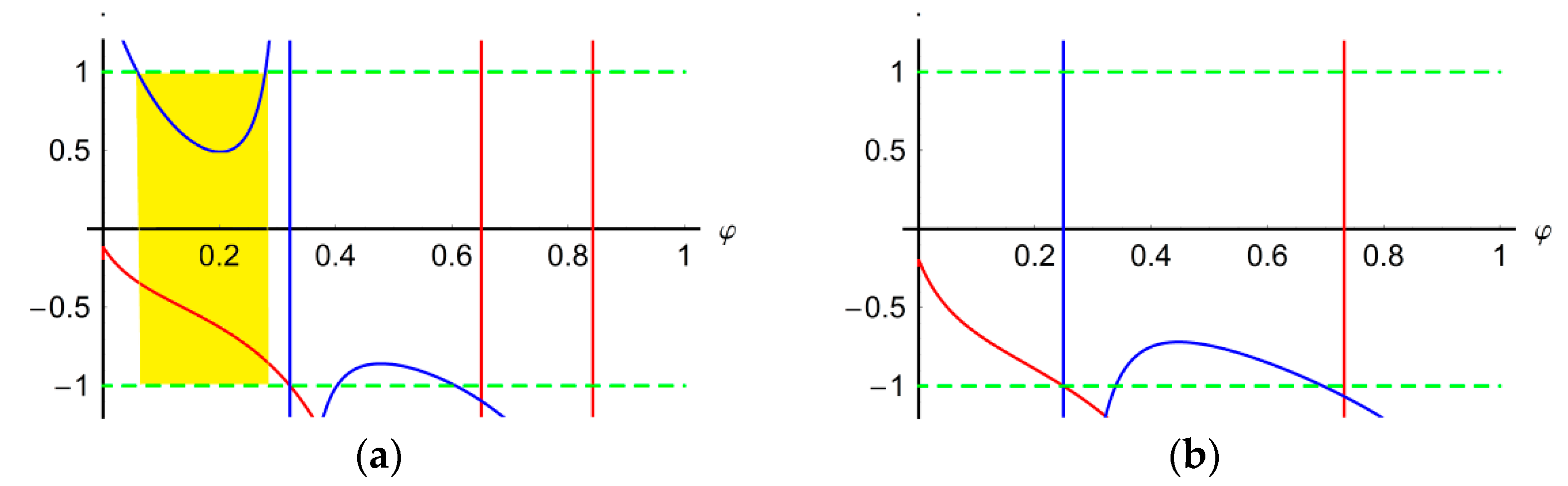
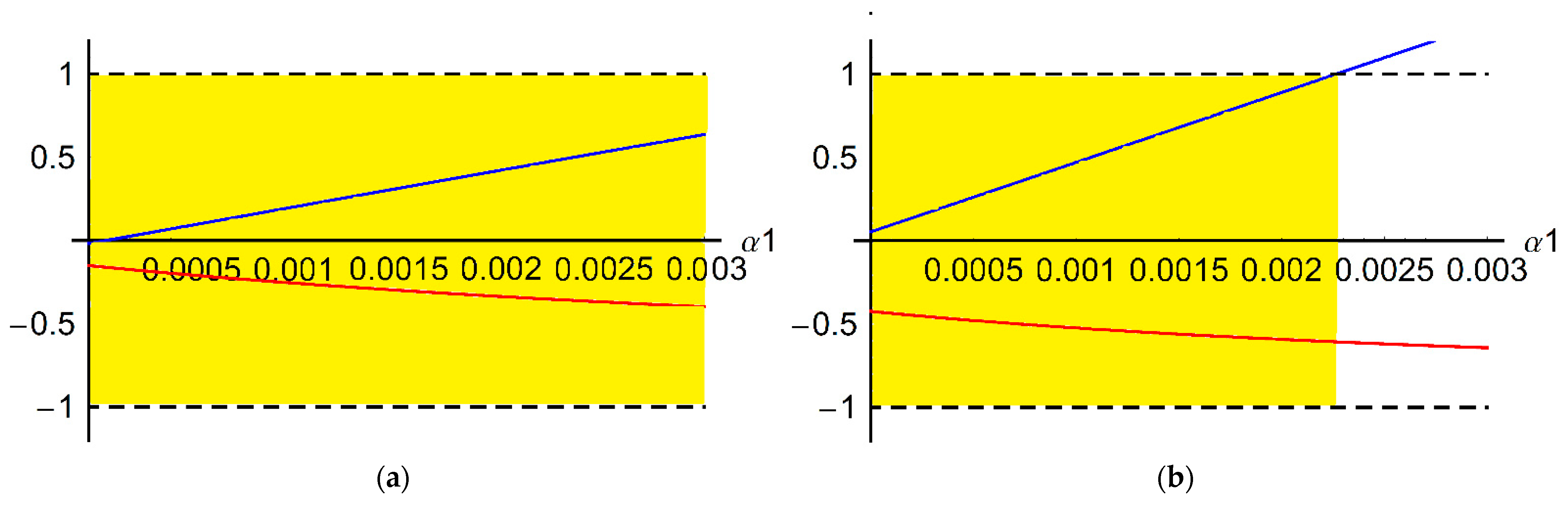
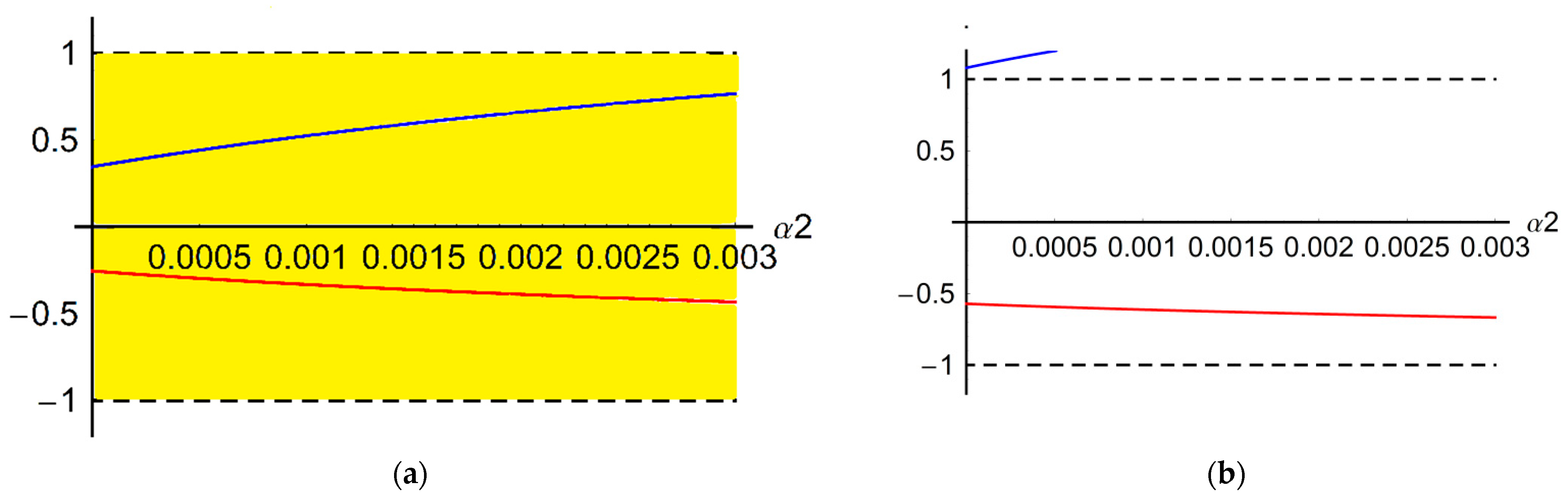
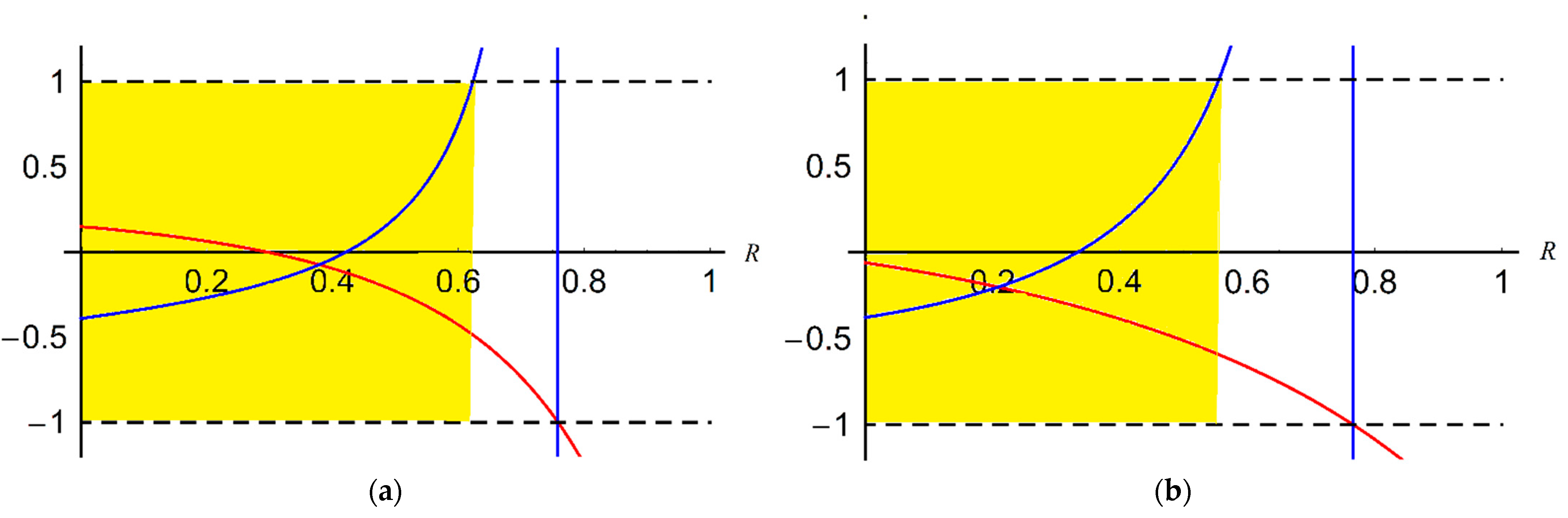
A graphical analysis of the stability conditions is presented in Figure 6, Figure 7, Figure 8 and Figure 9, taking into account the influence of different parameters; the yellow color denotes a zone of stability.

7. Conclusions

In this paper, we presented a study on the dynamical model of a two-degree-of-freedom vibro-impact oscillator with damping, subject to a perturbing force. Within this system, each of the masses may produce a combination of continuous movements or vibro-impact movements that are quite complicated. The system under study was composed of a linear oscillator and nonlinear one whose movements were determined by means of an approximate analytical solution, very close to the numerical solution. This approximate analytical solution was optimally determined using a new method, namely the Optimal Auxiliary Functions Method (OAFM), which was very efficient in practice. This solution was further used in analyzing the kinetic energy loss, the contact force, and the stability of periodic motions. Several cases were emphasized for possible movements of the system depending on the initial conditions and movement parameters, considering various impact possibilities between the two oscillators or between the oscillators and the walls.

In the case of periodic movements, it was considered that the period of the system was proportional with the period of the perturbing force. The boundary conditions of the system between two periodic subsequent arbitrary impacts were considered. After some analytical and numerical computations and by using the Schur principle, we established the stability conditions of the system. For different values of the movement parameters, a graphical analysis of stability conditions was presented. Different expressions for the velocities of the two oscillators were considered, establishing recurrence relations for periodic solutions.

Limitations of this study include the fact that it did not cover bifurcation- and chaos-related problems, but these aspects will be the subject of future developments. In addition, more research will be necessary to refine and further elaborate the proposed approach to make it applicable to three-degree-of-freedom vibro-impact systems, which would provide a more complete understanding of more complex systems. Moreover, as an alternative to the Schur criterion, use of the Zhukovsky-type stability [33] could be convenient, and the Sommerfeld effect [34,35] could be investigated by means of OAFM.

References

- Sayed, M.; Hamed, Y.S. Analytical, numerical solutions and study of stability, resonance for nonlinear vibro-impact system under different excitation. Int. J. Sci. Eng. Res. 2014, 5, 38–45. [Google Scholar]
- Askari, A.R.; Tahani, M. An alternative reduced order model for electrically actuated micro-beams under mechanical shock. Mech. Res. Commun. 2014, 57, 34–39. [Google Scholar] [CrossRef]
- Thomsen, J.J.; Fidlin, A. Near-elastic vibro-impact analysis by discontinuous transformations and averaging. J. Sound Vibr. 2008, 12, 386–407. [Google Scholar] [CrossRef][Green Version]
- Masri, S.F. Analytical and Experimental Studies of Impact Dampers. Ph.D. Thesis, California Institute of Technology, Pasadena, CA, USA, 1965. [Google Scholar]
- Kobrinski, A.Y. Mechanisms with Elastic Couplings. Dynamics and Stability; Nauka Press: Moscow, Russia, 1964. [Google Scholar]
- Babitsky, V.I. Theory of Vibro-Impact System and Applications; Springer: Berlin/Heidelberg, Germany, 1988. [Google Scholar]
- Brîndeu, L. Stability of the periodic motions of the vibro-impact systems. Chaos Solitons Fractals 2000, 11, 2493–2503. [Google Scholar] [CrossRef]
- Okolewska, B.B.; Czolczynski, K.; Kapitaniak, T. Dynamics of a two-degree-of-freedom cantilever beam with impacts. Chaos Solitons Fractals 2009, 40, 1991–2006. [Google Scholar] [CrossRef]
- Cronin, D.I.; Van, N.K. Substitute for the impact damper. J. Eng. Ind. 1975, 97, 1295–1300. [Google Scholar] [CrossRef]
- Shaw, S.W. The dynamics of a harmonically excited system having rigid amplitude constraints. J. Appl. Mech. 1985, 52, 453–458. [Google Scholar] [CrossRef]
- Ivanov, A.P. Analytical methods in the theory of vibro-impact systems. J. Appl. Mech. 1993, 57, 221–236. [Google Scholar] [CrossRef]
- Aziz, M.A.F.; Vakakis, A.F.; Manevich, L.I. Exact solutions of the problem of the vibro-impact oscillations of a discrete system with two degrees of freedom. J. Appl. Mech. 1999, 63, 527–530. [Google Scholar] [CrossRef]
- Luo, A.C.J. An unsymmetrical motion in a horizontal impact oscillator. J. Vibr. Acoust. 2002, 124, 453–458. [Google Scholar] [CrossRef]
- De Souza, S.L.T.; Caldas, I.L. Controlling chaotic orbits in mechanical systems with impact. Chaos Solitons Fractals 2004, 19, 171–178. [Google Scholar] [CrossRef]
- Emans, J.; Wiercigroch, M.; Krivtsov, A.M. Cumulative effect of structural nonlinearities: Chaotic dynamics of cantilever beam system with impact. Chaos Solitons Fractals 2005, 23, 1661–1670. [Google Scholar] [CrossRef]
- Mann, B.P.; Carter, R.E.; Hazra, S.S. Experimental study of an impact oscillator with viscoelastic and Hertzian contact. Nonlin. Dyn. 2007, 50, 587–596. [Google Scholar] [CrossRef]
- Avramov, K.V. Application of non smooth transformations to analyze a vibroimpact Duffing system. Int. J. Appl. Mech. 2008, 44, 1173–1179. [Google Scholar] [CrossRef]
- Bichri, A.; Belhaq, M.; Liaudet, J.P. Control of vibroimpact dynamics of a single-sided Hertzian contact forced oscillator. Nonlin. Dyn. 2010, 63, 51–60. [Google Scholar] [CrossRef]
- Grace, I.M.; Ibrahim, R.A.; Pilipchuk, V.N.P. Inelastic impact dynamics of ships with one-sided barriers. Part 1: Analytical and numerical investigations. Nonlin. Dyn. 2011, 66, 589–607. [Google Scholar] [CrossRef]
- Jovic, S.; Raicevic, V.; Garic, L. Vibro-impact system based on forced oscillations of heavy mass particle along a rough parabolic line. Math. Probl. Eng. 2012. [Google Scholar] [CrossRef]
- Lin, M.; Song, G.; Liu, Y.; Zhu, Y.; Zhang, X. Dynamic behavior analysis of vibro-impact system with two motion limited constraints. In Proceedings of the 4th International Conference on Mechanical and Manufacturing Engineering, Wuhan, China, 15–16 October 2016. [Google Scholar]
- Wang, J.; Shen, Y.; Yang, S. Dynamical analysis of a single degree-of-freedom impact oscillator with impulse excitation. Adv. Mech. Eng. 2017, 9, 1–10. [Google Scholar] [CrossRef]
- Reboucas, G.F.S.; Santos, I.E.; Thomsen, J.J. Unilateral vibro-impact systems-experimental observations against theoretical predictions based on the coefficient of restitution. J. Sound Vibr. 2019, 440, 346–371. [Google Scholar] [CrossRef]
- Fu, Y.; Quyang, H.; Davis, R.B. Nonlinear dynamics and triboelectric energy harvesting from a three-degree-of-freedom vibro-impact oscillator. Nonlin. Dyn. 2018, 92, 1985–2004. [Google Scholar] [CrossRef]
- Zukovic, M.; Hajradinovic, D.; Kovacic, I. On the dynamics of vibro-impact systems with ideal and non-ideal excitation. Meccanica 2021, 56, 439–460. [Google Scholar] [CrossRef]
- Marinca, V.; Herisanu, N. The nonlinear thermomechanical vibration of a functionally graded beam on Winkler-Pasternak foundation. MATEC Web Conf. 2018, 148, 13004. [Google Scholar] [CrossRef][Green Version]
- Herisanu, N.; Marinca, V. An effective analytical approach to nonlinear free vibration of elastically actuated microtubes. Meccanica 2021, 56, 813–823. [Google Scholar] [CrossRef]
- Marinca, V.; Herisanu, N. Optimal Auxiliary Functions Method for a pendulum wrapping on two cylinders. Mathematics 2020, 8, 1364. [Google Scholar] [CrossRef]
- Marinca, V.; Herisanu, N. Construction of analytic solutions to axisymmetric flow and heat transfer on a moving cylinder. Symmetry 2020, 12, 1335. [Google Scholar] [CrossRef]
- Herisanu, N.; Marinca, V. An efficient analytical approach to investigate the dynamics of a misaligned multirotor system. Mathematics 2020, 8, 1083. [Google Scholar] [CrossRef]
- Herisanu, N.; Marinca, V.; Madescu, G. Application of the Optimal Auxiliary Functions Method to a permanent magnet synchronous generator. Int. J. Nonlinear Sci. Numer. Simul. 2019, 20, 399–406. [Google Scholar] [CrossRef]
- Awrejcewicz, J.; Tomczak, K.; Lamarque, C.H. Controlling systems with impacts. Int. J. Bifurc. Chaos 1999, 9, 547–553. [Google Scholar] [CrossRef]
- Shiryaev, A.S.; Khusainov, R.R.; Mamedov, S.N.; Gusev, S.V.; Kuznetsov, N.V. On Leonov’s method for computing the linearization of transverse dynamics and analyzing Zhukovsky stability. Vestnik St. Petersburg Univ. Math. 2019, 52, 334–341. [Google Scholar]
- Dudkowski, D.; Jafari, S.; Kapitaniak, T.; Kuznetsov, N.V.; Leonov, G.A.; Prasad, A. Hidden attractors in dynamical systems. Phys. Rep. 2016, 637, 1–50. [Google Scholar] [CrossRef]
- Kiseleva, M.M.; Kondratyeva, N.; Kuznetsov, N.; Leonov, G. Hidden Oscillations in Electromechanical Systems; Springer: Cham, Switzerland, 2018. [Google Scholar]