Evaluating Popular Statistical Properties of Incomplete Block Designs: A MATLAB Program Approach

Abstract

Evaluating the statistical properties of a semi-Latin square, and in general, an incomplete block design, is vital in determining the usefulness of the design for experimentation. Improving the procedures for obtaining these statistical properties has been the subject of some research studies and software developments. Many available statistical software that evaluate incomplete block designs do so at the level of analysis of variance but not for the popular A-, D-, E-, and MV-efficiency properties of these designs to determine their adequacy for experimentation. This study presents a program written in the MATLAB environment using MATLAB codes and syntaxes which is capable of computing the A-, D-, E-, and MV-efficiency properties of any $\left(n\times n\right)/k$ semi-Latin square and any incomplete block design via their incidence matrices, where N is the number of rows and columns and k is the number of plots. The only input required for the program to compute the four efficiency criteria is the incidence matrix of the incomplete block design. The incidence matrix is the binary representation of an incomplete block design. The program automatically generates the efficiency values of the design once the incidence matrix has been provided, as shown in the examples.

1. Introduction

An $\left(n\times n\right)/k$ semi-Latin square, according to Bedford and Whitaker [1], Bailey and Royle [2] and Soicher [3], has N² cells (called blocks) in a square array, where each block has k plots, and there are Nk treatments which are allocated to plots such that each treatment occurs once in each row and once in each column (see also References [2,3]). Bailey [4] listed some methods for the construction of semi-Latin squares, such as the inflation method, interleaving method, Trojan method, superposition method, etc. Software such as the nauty package by McKay [5], GRAPE package by Soicher [6] and Traces package by McKay and Piperno [7] aid in the enumeration of semi-Latin squares up to isomorphism classification by exploring the graphical properties of the semi-Latin squares. Bailey and Royle [2] pointed out that results from graph theory can be applied to problems of incomplete block designs and the quotient block design of a semi-Latin square is said to be a regular-graph design.

A semi-Latin square could be referred to as an incomplete block design with the usual parameters, t, b, r, k and λ, where b is the number of blocks, r is the treatment replication while λ is the number of times each pair of treatments appears together in the design [2]. The most important statistical property of a block design is the efficiency, and there are many measures of efficiency of a block design, including the popular A-, D-, E-, and MV-efficiencies. According to John [8], incomplete block designs with equal block sizes often differ in the precision with which treatment effects are estimated, and efficiency factors of the incomplete block designs provide useful measures of these differences.

The efficiency factors, in particular, the pairwise and canonical efficiency factors, of incomplete block designs have been the subject of extensive research in the area of statistical analysis of incomplete block designs [8,9,10]. Most statistical efficiency measures of the incomplete block designs are derived from their pairwise/canonical efficiency factors. Bailey and Royle [2] and Morgan [11] stated that the A-, D- and E-efficiency measures are obtained from the canonical efficiency factors, while the MV-efficiency measure is obtained from the component of the pairwise efficiency factors. The canonical efficiency factors are the non-zero eigenvalues of the information matrix, while the pairwise efficiency factors are obtained from the variances of the treatment contrasts.

The earliest programs for incomplete block designs were built to analyze the isomorphism and automorphism properties of the $\left(n\times n\right)/k$ semi-Latin squares. Such programs include McKay’s nauty package and the program by Bailey and Royle [2], which runs on SparcStation ELC. The nauty package uses the graph properties of semi-Latin squares to obtain the isomorphism and automorphism classifications but does not evaluate the statistical properties of the semi-Latin squares, such as the optimality and efficiency properties. The nauty package is not easily accessible and runs only on a number of systems. The Bailey and Royle program was designed for only $\left(6\times 6\right)/2$ semi-Latin squares and also uses the orthogonal one-factorizations of the regular graph designs for the construction of the semi-Latin squares on SparcStation ELC, and each graph takes about one minute of CPU time. GRAPE software was developed by Soicher [6] in 1993, while the shipped version was developed in 2019. The GRAPE software runs partly on GAP environment and is primarily designed for constructing and analyzing graphs related to finite geometry, groups and designs. The other component runs on McKay’s nauty package. According to Soicher [12], the GRAPE algorithm performs more slowly and the computer time is not exact. The MATLAB program presented here utilizes simple matrix algebra, which is already part of the MATLAB codes and syntaxes, to obtain the four popular statistical properties, A-, D-, E-, and MV-efficiencies, of any incomplete block design in about one second of computer time.

The MATLAB R2019a software has an in-built statistics toolbox which is a collection of MATLAB codes and syntaxes for statistical data analysis. The statistics toolbox could analyze incomplete block designs up to analysis of variance tests of hypothesis but does not contain the required codes to obtain the A-, D-, E-, and MV-efficiencies measures of incomplete block designs. In this study, we provide a MATLAB program for the computation of the A-, D-, E-, and MV-efficiencies of incomplete block designs from their canonical and pairwise efficiency factors. The program, presented in the Appendix A, is capable of accurately computing the A-, D-, E-, and MV-efficiencies measures of any semi-Latin square, and in general, all incomplete block designs. The program requires only input of the binary equireplicate incidence matrix of the block.

2. Materials and Methods

2.1. Algebraic Basis for the Program

Given a semi-Latin square, $\Xi$, with $t=nk$ treatments arranged in $b=n^2$ blocks, the incidence matrix, N, emanating from $\Xi$ or that of any other t-treatment incomplete block design, $\Sigma$, in b blocks, is a $t\times b$ matrix of 1’s and 0’s. The $t\times t$ concurrence matrix of the incomplete block design is a product of N and its transpose, $N^{\prime }$. The concurrence matrix, $N{N}^{\prime }$, is then transformed to the information, $C=R-\left(\frac{1}{k}N{N}^{\prime }\right)$, of order t, where $R=rI$, r is the treatment replication in N and I is an identity matrix, also of order t. The product of the eigenvalues of C and the reciprocal of r gives the $t-1$ canonical efficiency factors, ${\omega }_i$, $i=1, 2, . . ., t-1$, of $\Xi$ or $\Sigma$, with one of the values of ${\omega }_i$ being equal to zero. Conversely, multiply C by the reciprocal of r to normalize the information matrix to obtain $C^{\ast }=I-\left(\frac{1}{rk}N{N}^{\prime }\right)$. Then, the canonical efficiency factors, ${\omega }_i$, are the $t-1$ non-zero eigenvalues of $C^{\ast }$.

The A-efficiency measure of $\Xi$ or $\Sigma$ is the harmonic mean of the canonical efficiency factors and is given by $A=\left(t-1\right){\left({\displaystyle \sum _{i=1}^{t-1}\frac{1}{{\omega }_i}}\right)}^{-1}$. The D-efficiency measure is the geometric mean of the canonical efficiency factors and is given by $D={\left({\displaystyle \prod _{i=1}^{t-1}{\omega }_i}\right)}^{1/t-1}$, while the E-efficiency is the minimum of the canonical efficiency factors, given by $E=\min \left({\omega }_i\right)$. The MV-efficiency measure is obtained from the components of the generalized inverse of C. Let $C_{inv}$ be the Moore–Penrose generalized inverse of C and ${\delta }_i$, $i=1, 2, . . ., t$, the i-th treatment effect, with ${\widehat{\delta }}_i$ the least squares estimator of ${\delta }_i$. Then, the treatment contrast is $\left({\widehat{\delta }}_i-{\widehat{\delta }}_j\right)$, $i\ne j$, while the variance from intra-block analysis of the incomplete block design is $\mathrm{var}\left({\widehat{\delta }}_i-{\widehat{\delta }}_j\right)$ = $\left({\xi }_{ii}+{\xi }_{jj}-2{\xi }_{ij}\right){\sigma }^2$, where ${\xi }_{ij}$ is the (i,j)-th element of $C_{inv}$. The MV-efficiency criterion is given as $\max \left\{\mathrm{var}\left({\widehat{\delta }}_i-{\widehat{\delta }}_j\right)\right\}$: see, for example, Reference [11].

2.2. Theoretical ComputatioN of the EfficieNcy Criteria

Given an incomplete block design, $\Sigma$(t, b, r, k λ), the $t\times b$ incidence matrix, N, has its (i, j) entry as the number of times treatment i occurs in block j. The column sums of N are all equal to the block size, k, and the sum of the i-th row, $r_i$, is the i-th treatment replication (that is, the number of times treatment i occurs overall). If $r_i$ is the same for all the treatments, then $\Sigma$(t, b, r, k λ) is called an equireplicate design. The matrix, N, is made binary by identifying treatment positions in each block by ‘1’ and non-treatment positions by ‘0’. Let $\Xi \in \Sigma \left(t,b,r,k,\lambda \right)$ be the $\left(6\times 6\right)/2$ semi-Latin square, ${\mathrm{\Delta }}_0$, of Bailey and Royle [2]. The design, ${\mathrm{\Delta }}_0$, is displayed in Figure 1. The input matrix required by this MATLAB program to compute the efficiency criteria of ${\mathrm{\Delta }}_0$ is the $12\times 36$ incidence matrix of ${\mathrm{\Delta }}_0$, given by N =

1	0	0	0	0	0	0	0	0	0	1	0	0	0	0	0	0	1	0	0	1	0	0	0	0	1	0	0	0	0	0	0	0	1	0	0
0	0	1	0	0	0	0	0	0	1	0	0	0	0	0	0	1	0	0	0	0	0	0	1	1	0	0	0	0	0	0	1	0	0	0	0
0	1	0	0	0	0	1	0	0	0	0	0	0	0	0	0	0	1	0	0	0	1	0	0	0	0	1	0	0	0	0	0	0	0	1	0
0	0	0	1	0	0	0	0	0	0	0	1	0	0	0	0	1	0	1	0	0	0	0	0	0	1	0	0	0	0	0	0	1	0	0	0
0	0	1	0	0	0	1	0	0	0	0	0	0	1	0	0	0	0	0	0	0	0	1	0	0	0	0	1	0	0	0	0	0	0	0	1
0	0	0	0	1	0	0	0	0	0	0	1	1	0	0	0	0	0	0	1	0	0	0	0	0	0	1	0	0	0	0	0	0	1	0	0
0	0	0	1	0	0	0	0	1	0	0	0	0	1	0	0	0	0	0	0	0	0	0	1	0	0	0	0	1	0	1	0	0	0	0	0
0	0	0	0	0	1	0	1	0	0	0	0	1	0	0	0	0	0	0	0	1	0	0	0	0	0	0	1	0	0	0	0	0	0	1	0
0	0	0	0	1	0	0	0	1	0	0	0	0	0	0	1	0	0	1	0	0	0	0	0	0	0	0	0	0	1	0	1	0	0	0	0
1	0	0	0	0	0	0	1	0	0	0	0	0	0	1	0	0	0	0	0	0	1	0	0	0	0	0	0	1	0	0	0	0	0	0	1
0	0	0	0	0	1	0	0	0	0	1	0	0	0	0	1	0	0	0	1	0	0	0	0	1	0	0	0	0	0	0	0	1	0	0	0
0	1	0	0	0	0	0	0	0	1	0	0	0	0	1	0	0	0	0	0	0	0	1	0	0	0	0	0	0	1	1	0	0	0	0	0

Figure 1. Semi-Latin square design, ${\mathrm{\Delta }}_0$.

The program gives the $12\times 12$ concurrence matrix from N by multiplying N by its transpose, $N^{\prime }$, to obtain $N{N}^{\prime }$ =

6	0	1	1	0	1	0	1	0	1	1	0
0	6	0	1	1	0	1	0	1	0	1	1
1	0	6	0	1	1	0	1	0	1	0	1
1	1	0	6	0	1	1	0	1	0	1	0
0	1	1	0	6	0	1	1	0	1	0	1
1	0	1	1	0	6	0	1	1	0	1	0
0	1	0	1	1	0	6	0	1	1	0	1
1	0	1	0	1	1	0	6	0	1	1	0
0	1	0	1	0	1	1	0	6	0	1	1
1	0	1	0	1	0	1	1	0	6	0	1
1	1	0	1	0	1	0	1	1	0	6	0
0	1	1	0	1	0	1	0	1	1	0	6

This concurrence matrix can be obtained from the program by entering the command, ‘NNP’, in the command window. To obtain the information matrix, C, the treatment replication, r = 3, is used to multiply the identity matrix of order 12 (which is available in MATLAB as ‘eye(12)’) to give the R matrix of order 12. The concurrence matrix multiplied by the reciprocal of k, the block size, is subtracted from R to give C =

3	0	−0.5	−0.5	0	−0.5	0	−0.5	0	−0.5	−0.5	0
0	3	0	−0.5	−0.5	0	−0.5	0	−0.5	0	−0.5	−0.5
−0.5	0	3	0	−0.5	−0.5	0	−0.5	0	−0.5	0	−0.5
−0.5	−0.5	0	3	0	−0.5	−0.5	0	−0.5	0	−0.5	0
0	−0.5	−0.5	0	3	0	−0.5	−0.5	0	−0.5	0	−0.5
−0.5	0	−0.5	−0.5	0	3	0	−0.5	−0.5	0	−0.5	0
0	−0.5	0	−0.5	−0.5	0	3	0	−0.5	−0.5	0	−0.5
−0.5	0	−0.5	0	−0.5	−0.5	0	3	0	−0.5	−0.5	0
0	−0.5	0	−0.5	0	−0.5	−0.5	0	3	0	−0.5	−0.5
−0.5	0	−0.5	0	−0.5	0	−0.5	−0.5	0	3	0	−0.5
−0.5	−0.5	0	−0.5	0	−0.5	0	−0.5	−0.5	0	3	0
0	−0.5	−0.5	0	−0.5	0	−0.5	0	−0.5	−0.5	0	3

which is also of order 12. Dividing C by r, the normalized information matrix is obtained as $C^{\ast }$ =

0.5	0	−0.0833	−0.0833	0	−0.0833	0	−0.0833	0	−0.0833	−0.0833	0
0	0.5	0	−0.0833	−0.0833	0	−0.0833	0	−0.0833	0	−0.0833	−0.0833
−0.0833	0	0.5	0	−0.0833	−0.0833	0	−0.0833	0	−0.0833	0	−0.0833
−0.0833	−0.0833	0	0.5	0	−0.0833	−0.0833	0	−0.0833	0	−0.0833	0
0	−0.0833	−0.0833	0	0.5	0	−0.0833	−0.0833	0	−0.0833	0	−0.0833
−0.0833	0	−0.0833	−0.0833	0	0.5	0	−0.0833	−0.0833	0	−0.0833	0
0	−0.0833	0	−0.0833	−0.0833	0	0.5	0	−0.0833	−0.0833	0	−0.0833
−0.0833	0	−0.0833	0	−0.0833	−0.0833	0	0.5	0	−0.0833	−0.0833	0
0	−0.0833	0	−0.0833	0	−0.0833	−0.0833	0	0.5	0	−0.0833	−0.0833
−0.0833	0	−0.0833	0	−0.0833	0	−0.0833	−0.0833	0	0.5	0	−0.0833
−0.0833	−0.0833	0	−0.0833	0	−0.0833	0	−0.0833	−0.0833	0	0.5	0
0	−0.0833	−0.0833	0	−0.0833	0	−0.0833	0	−0.0833	−0.0833	0	0.5

The canonical efficiency factors of $\Xi \in \Sigma \left(t,b,r,k,\lambda \right)$ are the non-zero eigenvalues of $C^{\ast }$, given by:${\underset{¯}{\omega }}^{\prime }=1.6340,\hspace{0.33em}1.6340,\hspace{0.33em}3.0,\hspace{0.33em}3.0,\hspace{0.33em}3.36,\hspace{0.33em}3.36,\hspace{0.33em}4.0,\hspace{0.33em}4.0,\hspace{0.33em}4.0,\hspace{0.33em}4.0,\hspace{0.33em}4.0$. Therefore, A = 0.4909, D = 0.5210, and E = 0.2723. The MV is obtained from the contrasts of the Moore–Penrose inverse of C, given by M =

1.8674	−0.4394	0.0379	−0.0417	−0.3712	0.1061	−0.4508	0.1061	−0.3712	−0.0417	0.0379	−0.4394
−0.4394	1.8674	−0.4394	0.0379	−0.0417	−0.3712	0.1061	−0.4508	0.1061	−0.3712	−0.0417	0.0379
0.0379	−0.4394	1.8674	−0.4394	0.0379	−0.0417	−0.3712	0.1061	−0.4508	0.1061	−0.3712	−0.0417
−0.0417	0.0379	−0.4394	1.8674	−0.4394	0.0379	−0.0417	−0.3712	0.1061	−0.4508	0.1061	−0.3712
−0.3712	−0.0417	0.0379	−0.4394	1.8674	−0.4394	0.0379	−0.0417	−0.3712	0.1061	−0.4508	0.1061
0.1061	−0.3712	−0.0417	0.0379	−0.4394	1.8674	−0.4394	0.0379	−0.0417	−0.3712	0.1061	−0.4508
−0.4508	0.1061	−0.3712	−0.0417	0.0379	−0.4394	1.8674	−0.4394	0.0379	−0.0417	−0.3712	0.1061
0.1061	−0.4508	0.1061	−0.3712	−0.0417	0.0379	−0.4394	1.8674	−0.4394	0.0379	−0.0417	−0.3712
−0.3712	0.1061	−0.4508	0.1061	−0.3712	−0.0417	0.0379	−0.4394	1.8674	−0.4394	0.0379	−0.0417
−0.0417	−0.3712	0.1061	−0.4508	0.1061	−0.3712	−0.0417	0.0379	−0.4394	1.8674	−0.4394	0.0379
0.0379	−0.0417	−0.3712	0.1061	−0.4508	0.1061	−0.3712	−0.0417	0.0379	−0.4394	1.8674	−0.4394
−0.4394	0.0379	−0.0417	−0.3712	0.1061	−0.4508	0.1061	−0.3712	−0.0417	0.0379	−0.4394	1.8674

The variances of the elementary treatment contrasts for $i\ne j$ are presented as ttt =

0	0.4335	0.5466	0.5238	0.4467	0.5677	0.4314	0.5677	0.4467	0.5238	0.5466	0.4335
0	0	0.4335	0.5466	0.5238	0.4467	0.5677	0.4314	0.5677	0.4467	0.5238	0.5466
0	0	0	0.4335	0.5466	0.5238	0.4467	0.5677	0.4314	0.5677	0.4467	0.5238
0	0	0	0	0.4335	0.5466	0.5238	0.4467	0.5677	0.4314	0.5677	0.4467
0	0	0	0	0	0.4335	0.5466	0.5238	0.4467	0.5677	0.4314	0.5677
0	0	0	0	0	0	0.4335	0.5466	0.5238	0.4467	0.5677	0.4314
0	0	0	0	0	0	0	0.4335	0.5466	0.5238	0.4467	0.5677
0	0	0	0	0	0	0	0	0.4335	0.5466	0.5238	0.4467
0	0	0	0	0	0	0	0	0	0.4335	0.5466	0.5238
0	0	0	0	0	0	0	0	0	0	0.4335	0.5466
0	0	0	0	0	0	0	0	0	0	0	0.4335

The minimum of the variances of the elementary contrasts for each treatment is 0.4314. Hence, MV is the maximum of the minimum contrasts, MV = 0.4314.

2.3. DescriptioN of the Program

The MATLAB software by Mathworks is designed to run on C, C++, and MATLAB programming languages. The MATLAB program presented in this work requires inputting only the incidence matrix of the incomplete block design as a matrix to obtain the results of the four efficiency criteria as output. Paste the program on the MATLAB Command Window from where the program will request for the input of the incidence matrix through the command prompt, ‘N = ’. Paste the incidence matrix of the desired incomplete block design at the command prompt and the results of the A-, D-, E-, and MV-efficiencies would be displayed immediately on the Command Window. Alternatively, input the incidence matrix row-by-row, with rows separated by semi-colons in a bracket, then press the ‘Enter’ key on the computer keyboard to display the results. Another method of running the program is through the MATLAB M-file console. Copy and paste the program on the M-file console for easy editing. After inputting the incidence matrix either as a matrix or row-by-row, press the ‘Run’ button on the M-file toolbar to display the results of the four efficiency values on the Command Window.

Generally, by providing input of the incidence matrix, the program automatically estimates the basic parameters of an incomplete block design: the number of treatments, t, number of blocks, b, block size, k, and number of treatment replications, r. These parameters are vital in the computation of the information matrix, normalized information matrix, etc. Like the Command Window of the MATLAB software, the MATLAB program presented here is interactive. By interactive, we mean the ability of the program to accept input of the incidence matrix of an incomplete block design using the computer keyboard by typing the incidence matrix row-by-row and separating the rows with semi-colons or importing already prepared incidence matrix from other environments, such as Excel spreadsheet, Notepad, etc., and pasting the matrix on the program’s input command prompt on the Command Window or the M-file console.

The program computes the A-efficiency using the command, A_efficiency = (t − 1)*(1/sum1). The D-efficiency is computed using the command, D_efficiency = (sum2)^(1/(t − 1)), while the E-efficiency is computed with the command, E1_Efficiency = min(caneffifactor(2:t,:)). The MV-efficiency criterion is computed using the program command, MV_efficiency = max(mve(1,:)).

We now highlight some of the advantages of the MATLAB program in the evaluation of incomplete block designs. The program utilizes computer time of about one second and occupies a small disc space of 911 bytes. These are obvious advantages when compared to Bailey and Royle’s [2] program for evaluating only $\left(6\times 6\right)/2$ semi-Latin squares, which takes about one minute of computer time and could only be executed on SparcStation ELC and the GRAPE package, which runs more slowly without definite computer time. The program is also designed to accept only the incidence matrix as its input (instead of multiple inputs), from which the parameters of the incomplete block designs are estimated by the program. The program computes the exact values of the four efficiency measures for any incomplete block design and does not give any approximate values for any of the efficiency measures. For instance, in the first illustrative example in Section 3.1, the program computed the exact values of some of those efficiency measures of the seven semi-Latin squares provided by Bailey and Royle [2] as approximate values.

3. Results

The MATLAB program, presented in the Appendix A, for the computation of the A-, D-, E-, and MV-efficiencies of incomplete block designs, including semi-Latin squares, completes the evaluation of any semi-Latin square or any other incomplete block design from the incidence matrix in less than one second of computing time on an HP Intel (R) Core (TM)i5–4200U CPU with 4.0 GB RAM in a 64-bit Operating System running on Windows. The program size is 911 bytes.

In the subsequent subsection, we provide some illustrative examples of the performances of the MATLAB program in evaluating semi-Latin squares.

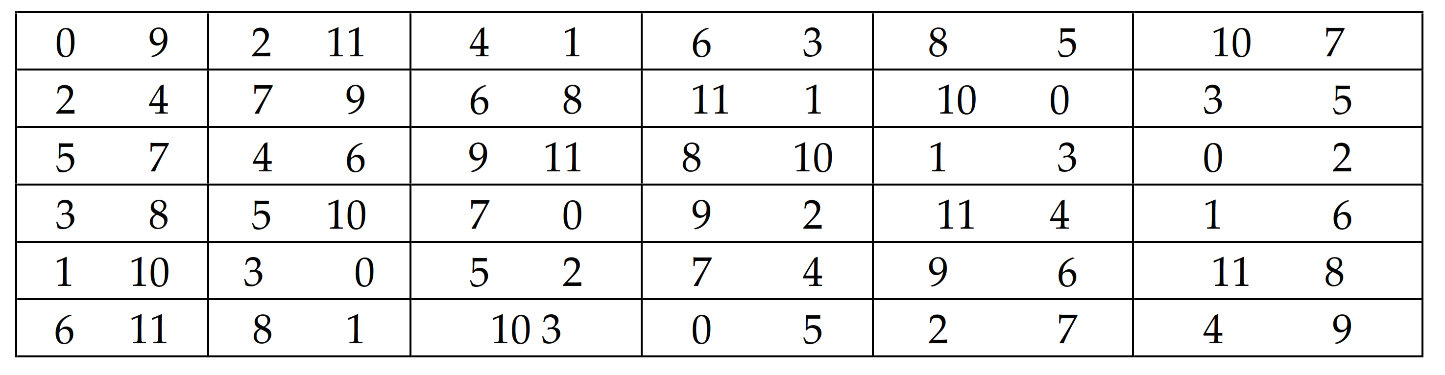
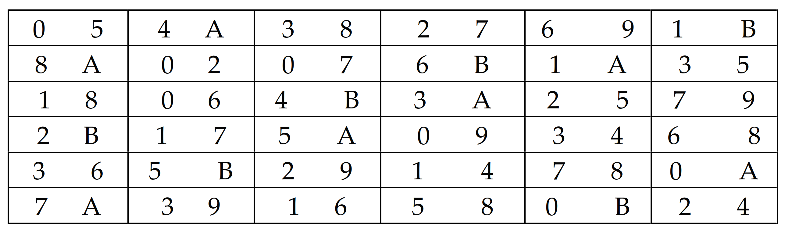
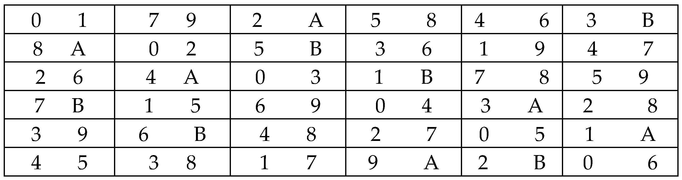
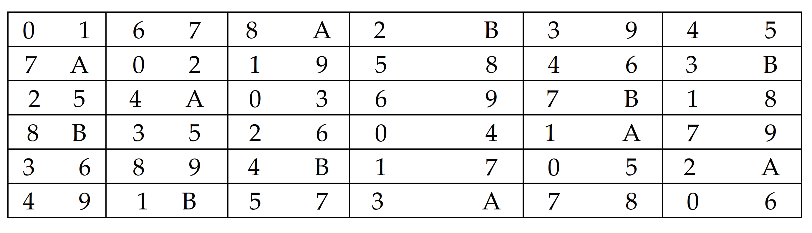
3.1. EvaluatioN of $\left(6\times 6\right)/2$ semi-LatiN squares (Bailey and Royle)

The first example is the computation of the A-, D-, E-, and MV-efficiency values of the seven $\left(6\times 6\right)/2$ semi-Latin squares, ${\mathrm{\Delta }}_0$, ${\mathrm{\Delta }}_1$, ${\mathrm{\Delta }}_2$, ${\mathrm{\Delta }}_3$, ${\mathrm{\Delta }}_4$, ${\mathrm{\Delta }}_5$, and ${\mathrm{\Delta }}_6$, constructed and evaluated by Bailey and Royle [2] using the graphical properties of the semi-Latin squares as quotient block designs. The semi-Latin squares are presented in Figure 1, Figure 2, Figure 3, Figure 4, Figure 5, Figure 6 and Figure 7 respectively, for ${\mathrm{\Delta }}_0$, ${\mathrm{\Delta }}_1$, ${\mathrm{\Delta }}_2$, ${\mathrm{\Delta }}_3$, ${\mathrm{\Delta }}_4$, ${\mathrm{\Delta }}_5$, and ${\mathrm{\Delta }}_6$. The corresponding efficiency values are presented in Table 1.

Figure 2. Semi-Latin square design, ${\mathrm{\Delta }}_1$.

Figure 3. Semi-Latin square design, ${\mathrm{\Delta }}_2$.

Figure 4. Semi-Latin square design, ${\mathrm{\Delta }}_3$.

Figure 5. Semi-Latin square design, ${\mathrm{\Delta }}_4$.

Figure 6. Semi-Latin square design, ${\mathrm{\Delta }}_5$.

Figure 7. Semi-Latin square design, ${\mathrm{\Delta }}_6$.

Table 1. Comparison of statistical efficiency values of the seven $\left(6\times 6\right)/2$ designs from our MATLAB program with the efficiency values in Bailey and Rolye [2].

S/N	The Design	Efficiency Values by Baileyand Royle [2]	Efficiency Values from Our MATLAB Program
1	${\mathrm{\Delta }}_0$	A-efficiency =        0.4909	A-efficiency =       0.4909
		D-efficiency =        0.5210	D-efficiency =       0.5210
		E-efficiency =        0.2723	E-efficiency =        0.2723
		MV-efficiency =    0.4314	MV-efficiency =     0.4314
2	${\mathrm{\Delta }}_1$	A-efficiency =        0.5133	A-efficiency =        0.5133
		D-efficiency =       0.5286	D-efficiency =        0.5286
		E-efficiency =        0.3333	E-efficiency =        0.3333
		MV-efficiency $\approx$   0.4444	MV-efficiency =   0.4633
3	${\mathrm{\Delta }}_2$	A-efficiency $\approx$     0.5129	A-efficiency =       0.5127
		D-efficiency $\approx$      0.5283	D-efficiency =       0.5281
		E-efficiency $\approx$       0.3759	E-efficiency =       0.3970
		MV-efficiency $\approx$   0.4619	MV-efficiency =    0.4783
4	${\mathrm{\Delta }}_3$	A-efficiency =        0.5127	A-efficiency =       0.5127
		D-efficiency =        0.5281	D-efficiency =       0.5281
		E-efficiency =        0.3970	E-efficiency =       0.3970
		MV-efficiency =     0.4783	MV-efficiency =    0.4783
5	${\mathrm{\Delta }}_4$	A-efficiency =        0.5100	A-efficiency =       0.5100
		D-efficiency =        0.5271	D-efficiency =        0.5271
		E-efficiency =        0.4167	E-efficiency =        0.4167
		MV-efficiency =     0.4688	MV-efficiency =     0.4688
6	${\mathrm{\Delta }}_5$	A-efficiency =        0.5115	A-efficiency =        0.5115
		D-efficiency =        0.5277	D-efficiency =        0.5277
		E-efficiency =         0.3865	E-efficiency =       0.3865
		MV-efficiency $\approx$    0.4675	MV-efficiency =    0.4692
7	${\mathrm{\Delta }}_6$	A-efficiency =        0.5127	A-efficiency =       0.5127
		D-efficiency =        0.5283	D-efficiency =       0.5283
		E-efficiency =         0.3494	E-efficiency =        0.3494
		MV-efficiency =     0.4559	MV-efficiency =    0.4743

From Table 1, the results of the MATLAB program show very high levels of accuracy in the computations of the A-, D-, E-, and MV-efficiencies of the $\left(6\times 6\right)/2$ semi-Latin squares. That is, the values of the four efficiency measures in Bailey and Royle [2] and from the MATLAB program presented here are exactly the same for most of the seven $\left(6\times 6\right)/2$ semi-Latin squares, except the approximate values. Additionally, the MATLAB program computed the exact values of the efficiency measures for some of the $\left(6\times 6\right)/2$ semi-Latin squares for which Bailey and Royle [2] could provide only the approximate values.

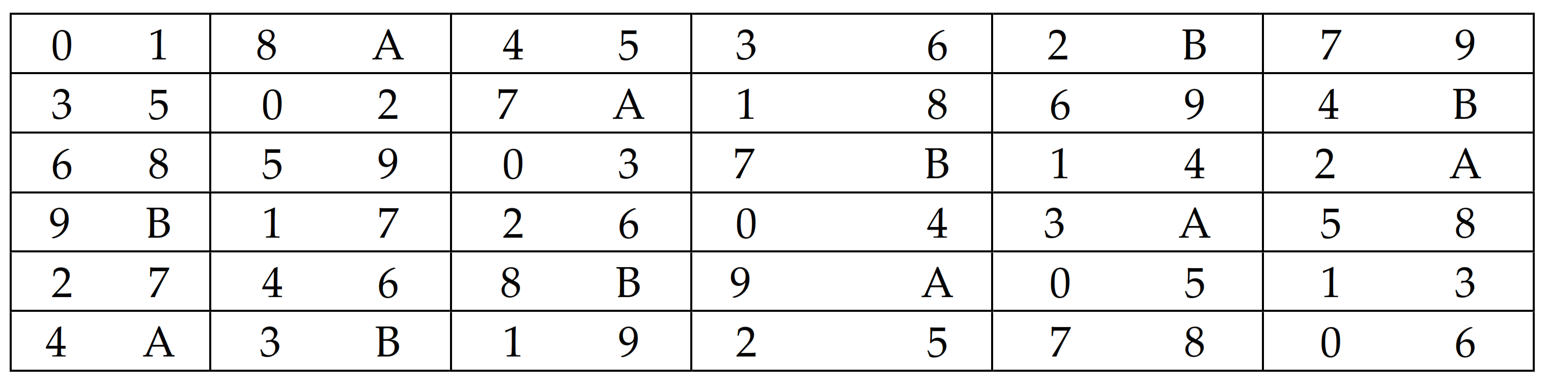
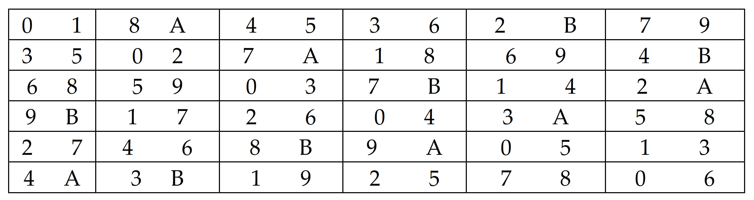
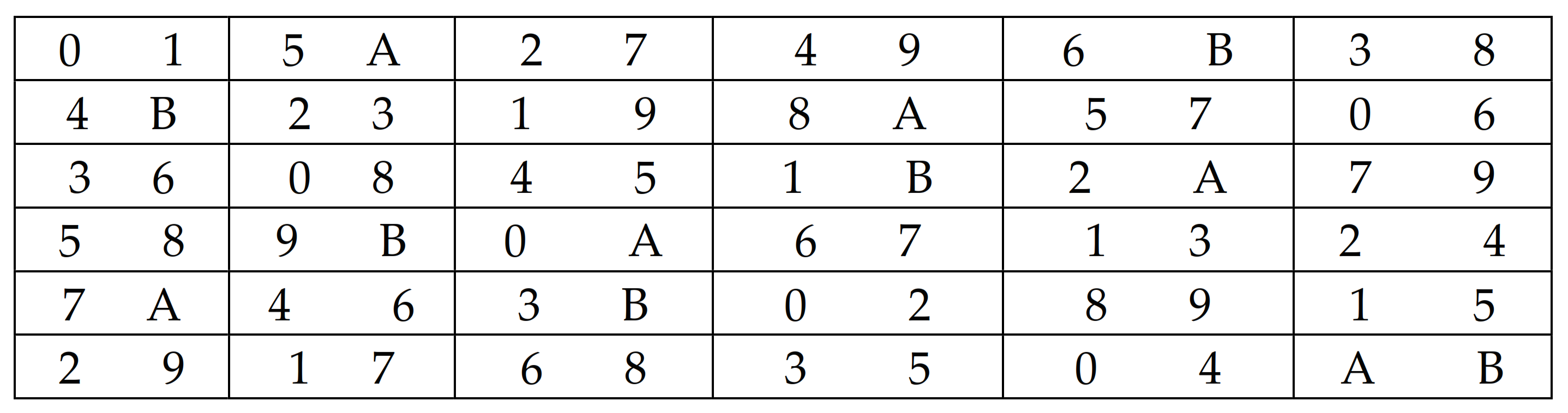
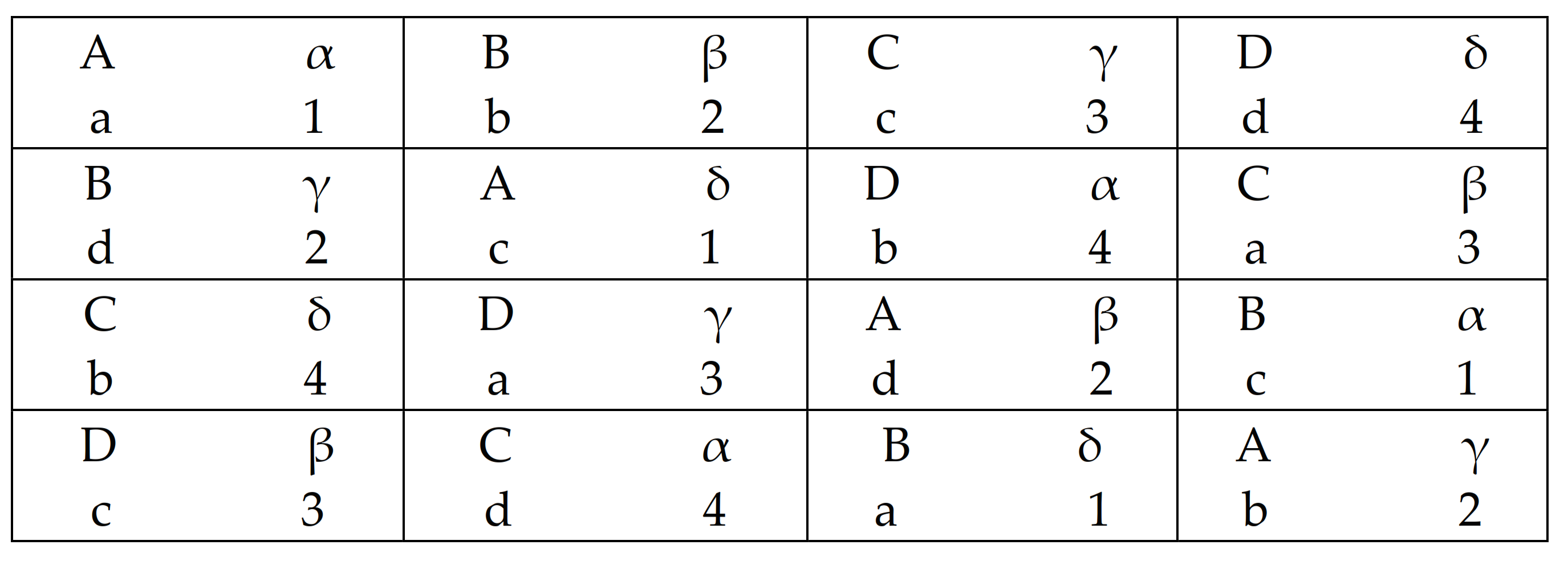
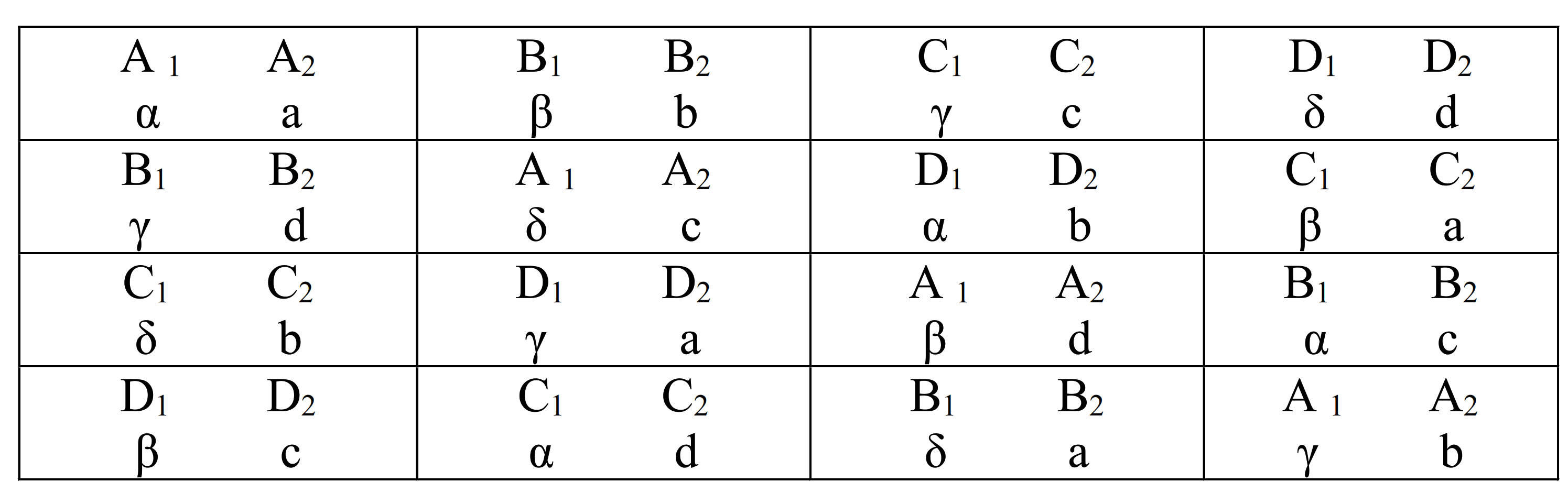
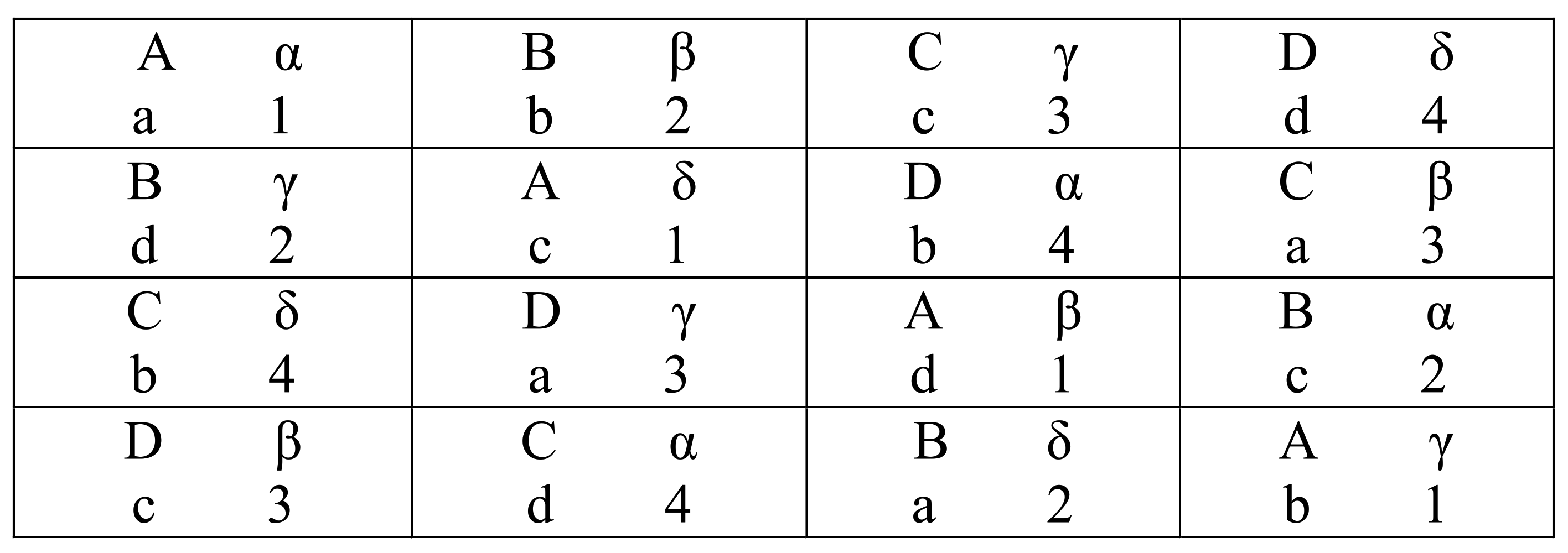
3.2. EvaluatioN of $\left(4\times 4\right)/4$ semi-LatiN square (Chigbu)

The second illustrative example for the use of the MATLAB program is in the evaluation of the three optimal $\left(4\times 4\right)/4$ semi-Latin squares whose statistical properties were studied by Chigbu [13]. The MATLAB program was used to obtain the values of the A-, D-, E-, and MV-efficiency measures of the three optimal $\left(4\times 4\right)/4$ semi-Latin squares. The three semi-Latin squares are ${\Omega }_1$, ${\Omega }_2$, and ${\Omega }_3$, and are presented in Figure 8, Figure 9 and Figure 10, while the results of their A-, D-, E-, and MV-efficiency measures are displayed in Table 2.

Figure 8. Semi-Latin square, ${\Omega }_1$.

Figure 9. Semi-Latin Square, Ω₂.

Figure 10. Semi-Latin square, ${\Omega }_3$.

Table 2. Comparison of the statistical efficiency values of the three $\left(4\times 4\right)/4$ semi-Latin squares from our MATLAB program with their efficiency values in Chigbu [13].

Design	Efficiency Criteria	Efficiency Values by Chigbu [13]	Efficiency Values from MATLAB Program
${\Omega }_1$	A	0.7500	0.7506
	D	0.7759	0.7761
	E	0.5000	0.5000
	MV	-	0.6667
${\Omega }_2$	A	0.7500	0.7500
	D	0.7759	0.7759
	E	0.5000	0.5000
	MV	-	0.7500
${\Omega }_3$	A	0.7500	0.7500
	D	0.7759	0.7759
	E	0.5000	0.5000
	MV	-	0.6667

Table 2 reveals that the A-, D- and E-efficiency values of ${\Omega }_2$ and ${\Omega }_3$ are exactly the same, while the three $\left(4\times 4\right)/4$ semi-Latin squares have exactly the same E-efficiency values. Slight differences exist between the values of A- and D-efficiencies of ${\Omega }_1$ and ${\Omega }_2$, which are attributable to what Soicher [3] referred to as mixture of manual and machine computations.

4. Discussion

In this work, the MATLAB program was presented for the evaluation of some statistical efficiency characteristics of any $\left(n\times n\right)/k$ semi-Latin squares, and in general, any incomplete block design using the design’s incidence matrix. To demonstrate the high level of accuracy of the program in computing the A-, D-, E-, and MV-efficiency measures of incomplete block designs, two illustrative examples were presented. The illustrative examples are the evaluations of the seven $\left(6\times 6\right)/2$ semi-Latin squares in [2] and the three optimal $\left(4\times 4\right)/4$ semi-Latin squares in [12]. Apart from giving exactly the same values for the four efficiency measures of the seven $\left(6\times 6\right)/2$ semi-Latin squares, the MATLAB program also provided exact efficiency values for some of the $\left(6\times 6\right)/2$ semi-Latin squares for which Bailey and Royle [2] could only provide approximate efficiency values. Specifically, the exact values of the MV-efficiency for ${\mathrm{\Delta }}_1$, A-, D-, E-, and MV-efficiencies for ${\mathrm{\Delta }}_2$ and MV-efficiency for ${\mathrm{\Delta }}_5$ were computed.

Furthermore, the MATLAB program dictated slight differences between the A- and D-efficiency values of the semi-Latin square, ${\Omega }_1$, and those of ${\Omega }_2$ and ${\Omega }_3$ in [12]. Additionally, the MV-efficiency measures of the three optimal $\left(4\times 4\right)/4$ semi-Latin squares which were not previously obtained by [12] were computed by the program. Using the minimum variance of the simple contrasts of the three optimal $\left(4\times 4\right)/4$ semi-Latin squares, Chigbu [13] concluded that ${\Omega }_2$ is preferable to ${\Omega }_1$ and ${\Omega }_3$. The results of the MV-efficiencies show that the value for ${\Omega }_2$ is higher than those for ${\Omega }_1$, and ${\Omega }_3$ reinforces that claim.

In general, the MATLAB program uses less than one second of computing time to compute and display the A-, D-, E-, and MV-efficiencies of any incomplete block design with a very high level of accuracy, as indicated in the illustrative examples.

References

- Bedford, D.; Whitaker, R. A New Construction for efficient semi-Latin squares. J. Stat. Plan. Inf. 2001, 9, 278–292. [Google Scholar] [CrossRef]
- Bailey, R.A.; Royle, G. Optimal semi-Latin squares with side six and block size two. Proc. Roy. Soc. 1997, 453, 1904–1914. [Google Scholar] [CrossRef]
- Soicher, L.H. Optimal and efficient semi-Latin squares. J. Stat. Plan. Inf. 2013, 143, 573–582. [Google Scholar] [CrossRef]
- Bailey, R.A. Semi-Latin squares. J. Stat. Plan. Inf. 1988, 18, 299–312. [Google Scholar] [CrossRef]
- McKay, B.D. Practical graph isomorphism. Cong. Numer. 1981, 30, 45–87. [Google Scholar] [CrossRef]
- Soicher, L.H. GRAPE: A system for computing with graphs and groups. In Groups and Computation; Larry, F., William, M.K., Eds.; American Mathematical Society: Providence, RI, USA, 1993; Volume 11, pp. 287–291. [Google Scholar]
- McKay, B.D.; Piperno, A. Practical Graph Isomorphism II. J. Sym. Comp. 2014, 60, 94–112. [Google Scholar] [CrossRef]
- John, J.A. Cyclic Designs; Springer-Science+Business Media, B.V.: Berlin/Heildeberg, Germany, 1987. [Google Scholar]
- John, J.A.; Williams, E.R. Cyclic and Computer Generated Designs; Springer-Science+Business Media, B.V.: Berlin/Heildeberg, Germany, 1995. [Google Scholar]
- Hinkelmann, K.; Kempthorne, O. Design and Analysis of Experiments; John Wiley and Sons Inc.: Hoboken, NJ, USA, 2005; Volume 2. [Google Scholar]
- Morgan, J.P. Blocking with independent responses. In Handbook of Design and Analysis of Experiments; Dean, A., Morris, M., Stufken, J., Bingham, D., Eds.; Chapman and Hall/CRC Press: Boca Raton, FL, USA, 2015. [Google Scholar]
- Soicher, L.H. The GRAPE Package for GAP. 2019. Available online: https://www.gap-system.org/Manuals/pkg/grape-4.8.3/doc/manual.pdf (accessed on 19 May 2021).
- Chigbu, P.E. The “Best” of the three optimal (4 × 4)/4 semi-Latin squares. Sankhya Indian J. Stat. 2003, 65, 641–648. [Google Scholar]
Publisher’s Note: MDPI stays neutral with regard to jurisdictional claims in published maps and institutional affiliations. |
© 2021 by the authors. Licensee MDPI, Basel, Switzerland. This article is an open access article distributed under the terms and conditions of the Creative Commons Attribution (CC BY) license (https://creativecommons.org/licenses/by/4.0/).