1. Introduction
New energy vehicles is defined as four-wheel vehicles using alternative fuel sources as the power source instead of conventional oil and gas, which includes hybrid vehicle (HV), battery electrical vehicle (BEV), fuel cell electric vehicle (FCEV), hydrogen engine vehicle (HEV), dimethyl ether vehicle (DEV), and other new energy (e.g., high-efficiency energy-storage devices) vehicles. Facing the increasing energy and environmental pressures, the development of new energy vehicles (NEVs) has become an accessible way to save energy and to reduce emissions. The NEV industry is in an infancy and incubation period in recent years. The report released by global market research organization “Energy Trend” shows that the global NEV sales accounted for only 1% of the total vehicle market and expected to grow up to 5% of total global vehicle sales by 2020 (
https://www.credenceresearch.com/report/new-energy-vehicles-market, (accessed on 21 March 2021)). Many countries announce policies to encourage the development of environmentally friendly vehicle technologies and to accelerate the marketization process of NEVs [
1,
2]. There are two main types of policies that are widely used to promote the development of NEVs, i.e., demand subsidy and production regulation.
The demand subsidy policies mainly provide preferential and convenience for consumers to purchase and use NEVs [
3]. For example, in the U.S., individuals and businesses who purchase NEVs in 2010 and after that year can obtain tax benefits from USD 2500 to USD 7500 based on the energy in the battery [
4]. In Norway, local NEV owners enjoy great benefits and conveniences, including free parking, lower annual license fees, exemption from import duties, etc. [
5,
6].
Regulation policies require manufacturers to increase the output of NEVs and to tighten emission standards of fuel vehicles (FVs). California is the first region to implement the “Zero Emission Vehicles (ZEV)” mandate to regulate vehicle manufacturers, which set an “energy credit” for each NEV and stipulates that the energy credits of NEVs must account for a percentage of the total output [
7,
8]. Upon failure to meet the requirements, the vehicle manufacturer must pay a fine of USD 5000 per energy credit to the government [
7,
8]. Similarly, China proposes a dual-credit policy for the automobile industrial on the production standard of NEVs and FVs. The dual-credit policy consists of the corporate average fuel consumption credit (CAFC-credit) rules, which set targets for the average energy consumption rate for FVs, and the new energy vehicle credit (NEV-credit) rules, which stipulate energy credits by NEV type and require certain NEV energy credit quotas. Manufacturers can achieve targets by producing NEVs or by purchasing energy credit from the energy credit trading market. By establishing an energy credit trading mechanism, manufacturers are encouraged to follow the production regulation standard. For example, nearly USD 190 million of Tesla’s profit was earned by selling energy credits in Q3, 2018 (
https://www.thedrive.com/news/24659/nearly-190m-of-teslas-q3-profit-was-earned-by-selling-regulatory-credits-not-sales-revenue, (accessed on 21 March 2021)). On the other hand, the SAIC General Motors Company would cost 28 million to 42 million yuan to purchase energy credit upon failure to meet the production regulation standard.
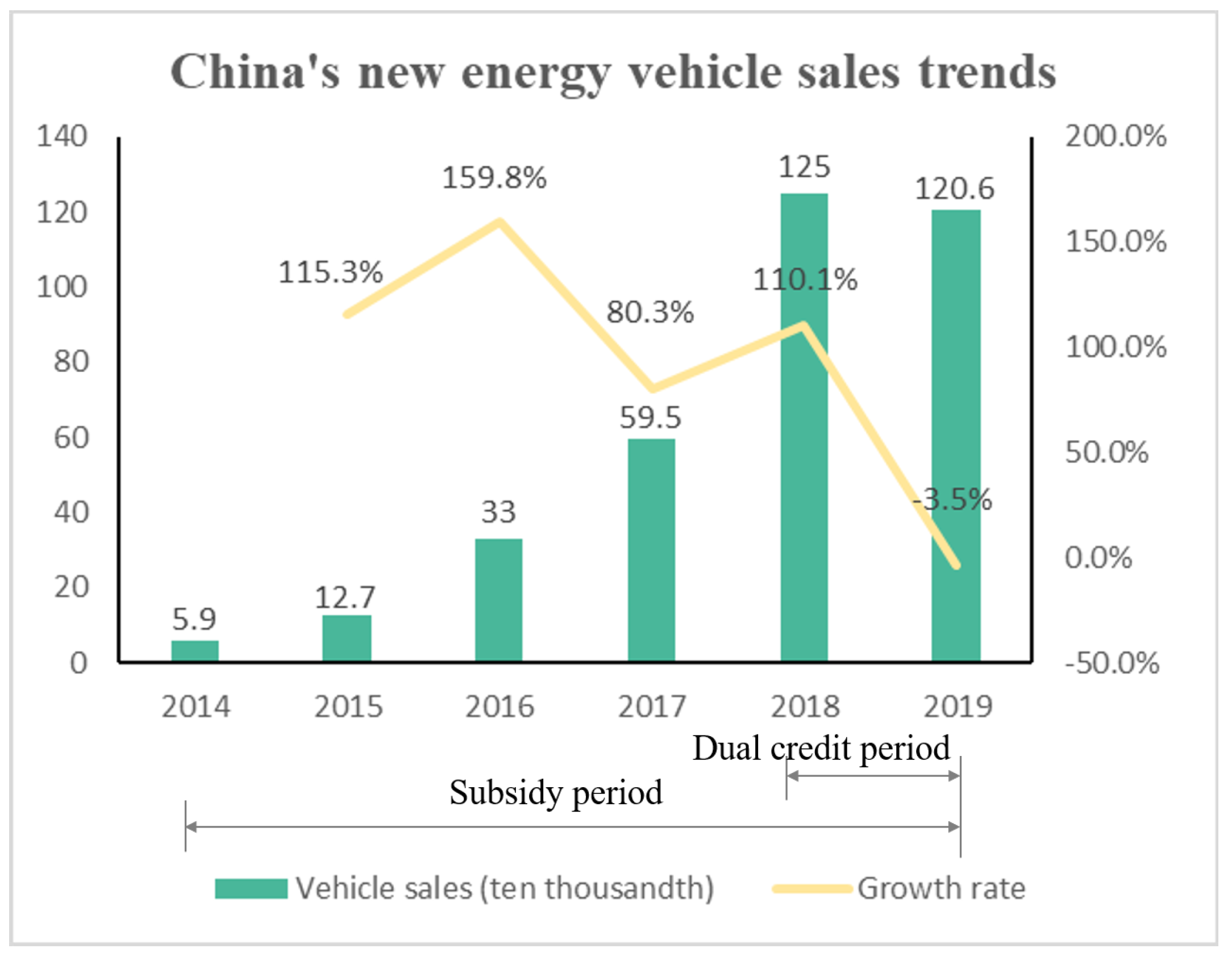
China, as the world largest vehicle market, implemented the demand subsidy and production regulation policies from 2010 and 2018, respectively. The demand subsidy policies were confirmed effectively in promoting the rapid development of NEVs [
9,
10]. For example, since the Chinesegovernment introduced subsidy policy for NEV buyers when they purchase or enjoy free parking and charging, the sales of NEVs increased rapidly from 2014 to 2018 (see
Figure 1), which also led to steady growth in overall vehicle sales from 2012 to 2017 (see
Figure 2). However, it is interesting to note that the implementation of a dual-credit policy made a difference to the vehicle market. The overall vehicle sales slumped after the rapid growth in China in 2018. Moreover, the sales growth rate of NEVs also declined in 2019 after four years of rapid increase. Therefore, based on the observation from reality, we develop a model to explore the reasons behind these phenomena. When promoting the development of NEVs, how does demand subsidies and production regulation affect the optimal production decisions of manufacturers? Moreover, the purpose of promoting NEVs needs not only to protect the environment but also to consider the overall impact on consumers, manufacturers, and society. Hence, the social planner’s optimal decision when formulating corresponding policies considering social welfare and environmental impact are also worth studying further.
In this paper, we investigate the following research questions: (i) What are the impacts of the two types of policies on the NEV adoption process, including price, quantity, and profit of manufacturers? (ii) What is the optimal decision of a social planner that helps achieve the adoption of NEVs and balanced objectives for maximizing social welfare and controls the environmental impact in the NEV market? To answer these questions, we construct a Stackelberg game with a welfare-maximizing policymaker and two profit-maximizing firms competing in the vehicle market. Considering the economic and environmental performances, consumers are assumed to have a preference for environmental attributes and are sensitive to price. By use of backward induction analysis, the optimal price, quantity of each type of vehicle, and the profit of firms are derived under three scenarios, that is, benchmarks without social planner intervention, with demand subsidy policy, and with production regulation policy, respectively. Then, the optimal decision of social planner is derived.
Our results provide several insights. Interestingly, although both types of policies can increase the quantity of NEVs, demand subsidy also promotes the growth of total vehicles at the same time; in contrast, production regulation reduces the number of total vehicles. Moreover, compared with the benchmark without policy intervention, demand subsidy generally improves social welfare, whereas production regulation benefits social welfare only when consumers show a high preference for NEVs. Nevertheless, production regulation always has a positive impact on the environment, whereas demand subsidy may have a positive impact only when the NEV is very environment friendly. The numerical results show that two parameters, consumer environmental preferences and the regulation of environmental impact, determine which type of policy dominates the other, i.e., meets the environmental impact regulation and achieves more social welfare simultaneously.
The remainder of this paper is organized as follows. A brief review of the related research paper is presented in
Section 2. In
Section 3, we present model assumptions and descriptions and show the optimal quantity, price, and profit of two manufacturers under three scenarios. In
Section 4, we focus on the optimal decision of a social planner with the goal of maximizing social welfare under environmental impacts constraints. Then, we present a numerical experiment to further explore the characteristics of the two types of policies. Finally, we discuss the managerial implications of our study and possible future work in
Section 6.
2. Literature Review
Our work builds on and contributes to previous literature on sustainable operations, economics, and operations management in the vehicle field. Therefore, the literature reviewed here primarily relates to two streams of research: (i) the effect of NEV-promoting policies on the manufacturer’s production decision, and (ii) the impact of adopting NEVs on environmental and socioeconomic performance.
Most research concentrates on demand subsidy policies that target the financial incentives such as purchase subsidies, fuel subsidies, and nonfinancial incentives such as free parking and high-occupancy vehicle lane access [
11]. From the perspective of the supply chain, several research confirmed that subsidies have a positive role in promoting the development of electric vehicles (EVs). Huang et al. constructed a duopoly model under a government’s subsidy incentive scheme, including an FV supply chain and an EV–FV supply chain. They concluded that a subsidy incentive scheme can help improve social welfare, can increase the sales of NEVs, and can reduce environmental hazards [
9]. After that, Luo et al. investigated an automobile supply chain consisting of one supplier and one retailer serving heterogeneous customers [
12]. Shao et al. compared the effectiveness of the subsidy scheme and the price discount incentive plan under two different structures: monopoly and duopoly. The consumers’ low-carbon awareness was also taken into account [
10]. However, some research showed that subsidies are not significant for the development of EVs. Han et al. presented that the implementation of the EV Subsidy Scheme in China did not successfully promote EV market presentation due to technical limitations of Li-ion batteries for EVs [
13]. Diamond found that the subsidy policy and the adoption of EV show a weaker relationship [
14]. Moreover, subsidies to promote the application of green technologies in the supply chain have also been confirmed by Wang et al. [
15].
To make up for the shortcomings of financial burden caused by subsidies, the production regulation policies are proposed to compulsorily regulate the production decision of manufacturers [
16]. Production regulation mainly refers to policies that require manufacturers to tighten emission standards of fuel vehicles (FVs), such as the Corporate Average Fuel Economy(CAFE) standard, and to increase the output of NEVs, such as California’s ZEV mandate and dual-credit policy. To comply with the CAFE regulation, Al-Alawi and Bradley showed that plug-in hybrid electric (PHEV) have advantages that save costs compared to conventional technologies [
17]. Sen et al. revealed that the CAFE regulation is indeed an effective policy solution that does increase the adoption of EVs, whether implemented alone or in conjunction with another policy, e.g., government incentives [
18]. Moreover, ZEV regulation and dual-credit policy also contribute to the output of NEVs. Greene et al. pointed out that ZEV regulation plays an important role in achieving the transition to EVs despite the market’s many uncertainties [
19]. Zhou et al. examined the impact of the dual-credit system on green technology investment and pricing decisions in a two-echelon supply chain [
20]. Compared with demand subsidy, Li et al. showed that the dual-credit policy can effectively promote the development of NEVs [
21]. Furthermore, Li et al. studied the subsidy policy and dual-credit policy on NEV and conventional vehicle (CV) production decisions from an across-chain perspective. CVs refer to four-wheel vehicles using conventional oil and gas as the source of power. They found that the dual-credit policy can improve the profit of NEV manufacturers and the total supply chain profit with the optimal credit price [
22]. Although the impact of the dual-credit policy on manufacturers’ decisions has been studied, our paper focuses on the impact of production regulation from the perspective of the social planner with the goal of maximizing social welfare and controlling the environmental impact in the vehicle market.
As for the study related to the environmental impact of NEVs, early researches found that the adoption of NEVs can significantly reduce greenhouse gas emissions such as carbon dioxide, which is beneficial to the environment [
23,
24]. Over time, much research extended the assessment of the environmental impact of NEVs to the entire life-cycle from exploitation to utilization. Faria et al. presented an environmental and economic Life-Cycle Assessment for conventional and NEV technology [
25]. However, some studies found that NEVs may not be as environmentally friendly as people think. Wu and Zhang pointed out that the impact of using NEVs on the environment should be considered from the perspective of the entire life cycle consisting of the process of exploitation, production, and utilization of energy and further proposed that the different utilization rates of energy in developed and developing countries lead to different effects [
26].
In general, existing studies have established a mature framework for NEV industry policies. However, there is a lack of studies on the comparative analysis of the demand subsidy and production regulation in the competitive environment, especially from the perspective of the decision of a social planner. Therefore, by constructing a duopoly model, we compare the production decision under production regulation and demand subsidy scenario. In addition, the social planner’s optimal decisions are also considered.
3. Model Description
We consider two competing manufacturers, and , which produce and sell the NEVs and FVs, respectively. The two manufacturers and simultaneously choose product prices and to maximize their profits. Due to the expensive cost of batteries, the unit production cost of the NEV is higher than that of the FV, i.e., . Without loss of generality, we assume that the unit cost of FV is normalized to zero (this assumption is not essential and is for convenience; our result remains valid under ).
We assume consumer heterogeneity with respect to the consumer willing-to-pay for FVs and NEVs. Denote
as the consumer’s valuation for purchasing the FV, which is subject to a uniform distribution from
. Considering that the NEV brings extra green utility
to consumers [
27], we obtain the valuation for purchasing the NEV as
, which is widely used, such as in Shao et al. [
10].
Table 1 summarizes the key notations in our following model development.
The sequence of the three-stage Stackelberg game is as follows: first, the social planner acts as the leader to set the per unit subsidy or production regulation standard to maximize social welfare. Then, depending on the subsidy or the regulation standard, the manufacturer decides the optimal retail price to maximize their profits. Finally, consumers choose to buy the NEV/FV or to remain inactive.
Next, we explore the impact of different types of policies on the promotion of NEVs. According to backward induction, we first consider the second stage for the manufacturer’s decision. To evaluate the performance of different types of policies, we first seek the scenario without social planner intervention as a benchmark in the next section.
3.1. The Basic Scenario
In the basic scenario, two competing manufacturers decide the retail price
of the NEV and FV simultaneously to maximize their profits without social planner involvement. We use superscript
B to represent the basic scenario. First, we analyze the consumers’ optimal strategies with the given retail prices to derive the demand functions of NEVs and FVs. Consumers face three choices, i.e., buy a NEV, buy a FV, or remain inactive. Denote
as the utility function of buying a NEV (or a FV, or to remain inactive); then, the three utilities for consumers is shown as follows:
Suppose that the consumer is rational, that is, the consumer chooses a product with higher nonnegative net utility. For example, a consumer with
and
buys the NEV and a consumer with
and
buys the FV. We set the boundary between the purchase of the FV and the NEV to
, which yields from Equation (
1). Similarly, the indifference point for buying a FV and not buying is
. With these conditions, given the specific retail price, each manufacture’s sales quantity in the basic scenario is specified in
Table 2.
Base on the demand function, the decision problem faced by manufacturer
is
and the decision problem faced by manufacturer
is
where
and
denote the quantity of NEVs and FVs determined by the selling price, respectively.
Proposition 1. For the basic scenario, the optimal decision of manufacturers and are as follows:
- (1)
if , manufacturer quits the market and manufacturer posts the optimal price ;
- (2)
if , manufacturer quits the market and manufacturer posts the optimal price ; and
- (3)
if , both firms compete in the market and set the optimal price .
All of the proofs are provided in
Appendix A. Proposition 1 shows that the equilibrium state is determined by the unit production cost of the NEV. When the unit production cost of NEV is high enough, i.e.,
, due to the cost advantages (
), manufacturer
always provides a lower price than that offered by manufacturer
to obtain profits as long as
. Thus, manufacturer
dominates the market with the price
. Manufacturer
cannot enter the market successfully. As technology advances, the production cost of NEVs declines (
), i.e., the NEV has the potential to enter the market [
28]. However, to resist the entry of the NEV, manufacturer 2 sets a lower price for the FV to force the NEV out of the market, i.e.,
. The price of a FV is already lower than the cost of a NEV, i.e.,
. To compete with manufacturer
, if manufacturer
adopts a price lower than the production cost, the marginal profit is negative, so the only choice is to quit the market. Although manufacturer
still monopolizes the market, its profit is lower than before due to the impact of the NEV (see
Table 3 for detail).
When the unit production cost of the NEV is further reduced, i.e.,
, the NEV successfully enters the market and sets price
. Wu et al. showed that the NEV can become more economic than FVs after 2025, which provides technical support and theoretical basis for the full popularity of the NEV [
29]. In this case, even if the price of the NEV is higher than that of the FV, some consumers still choose the NEV owning to consumers’ environmental preferences. Compared with the FV monopoly case, some customers move to buy the NEV, which results in the loss of customers for manufacturer
. As a response, manufacturer
raises prices to fully extract consumer surplus. The optimal quantity, price, and profit of manufacturer
and manufacturer
in the benchmark scenario are shown in
Table 3 and
Table 4, respectively.
3.2. The Demand Subsidy Scenario
Under the demand subsidy scenario, the social planner provides certain subsidies for consumers at the time of purchasing the NEV or brings convenience for using the NEV to improve the consumers’ satisfaction, such as free parking or special license plate to get on the road. Hence, consumers have extra utility
s when choosing a NEV. In this scenario, the consumer also has three options: buy a NEV, buy a FV, or remain inactive. The utility function of the customer is as follows:
where the utility function for buying a FV and remaining inactive are the same as Equation (
1). Similar to the previous section, consumers aim at maximizing their nonnegative utility. Based on the above information, the demand function for NEVs and FVs are shown in
Table 5.
Therefore, the problem of manufacturer
and manufacturer
can be described as follows:
Proposition 2. For the demand subsidy scenario, when the subsidy is given, the optimal decision of manufacturers and are as follows:
- (1)
if , then manufacturer quits the market and manufacturer posts the optimal price ;
- (2)
if , then manufacturer quits the market and manufacturer posts the optimal price ;
- (3)
if , both manufacturers exist in the market, then
;
- (4)
if , then manufacturer quits the market and manufacturer posts the optimal price ; and
- (5)
if , then manufacturer quits the market and manufacturer posts the optimal price ,
where , , , .
When the subsidy is very low, i.e., , such an inefficient subsidy cannot compensate for the disadvantages of high unit production costs of the NEV. Thus, manufacturer dominates the market with the FV and posts price . As the subsidy increases, i.e., , to resist the entry of the NEV, manufacturer sets price . Compared with the basic scenario, the implement of demand subsidy policies forces manufacturer to deal with a more serious market crisis, so they cut prices more than before, i.e., , resulting in an increase in the quantity of FVs, i.e., . In this case, it is worth noting that the incentive not only fails to promote the NEV but also indirectly increases the quantity of the FV.
As the subsidy further increases, manufacturer
enter the market to compete with manufacturer
. As the incentive continues to increase, the advantage of manufacturer
pushing manufacturer
out of the market grows. Even if manufacturer
sets the price of an FV to 0, the consumer still chooses a NEV instead of a FV due to their environment preferences. Finally, when the subsidy is very high, i.e.,
, manufacturer
dominates the market with price
. Thus, a relatively high price is drawn to fully extract the consumer surplus. The optimal quantity, price, and profit of manufacturer
and manufacturer
in the demand subsidy scenario are shown in
Table 6 and
Table 7, respectively.
Proposition 3. When NEVs and FVs both exist in the market, i.e., ,
the optimal price and quantity of the NEV both increases with the incentive. Thus, the profit of manufacturer increases with incentive, i.e., , , ;
the optimal price and quantity of the FV both decrease with the incentive. Thus, the profit of manufacturer decreases with incentive, i.e., , , ; and
the total quantity of vehicles in the market is larger than that of basic scenario, i.e., .
Proposition 3 states that, when NEVs and FVs both exist in the market, manufacturer produces more NEVs and manufacturer produces less FVs with higher subsidy, which is consistent with our intuition. Furthermore, consumers’ utility increases with higher incentive, which indicates consumers are more willing to pay for the NEV. Thus, manufacturer posts higher retail prices for NEVs. Conversely, manufacturer cuts the prices of FVs to attract consumers. With the increase incentived, the profit of manufacturer increases while the profit of manufacturer decreases. Furthermore, from , we can obtain that the growth rate of the NEVs is greater than the decline rate of the FV. Hence, demand subsidy always increases the total quantity of vehicles on the market.
3.3. The Production Regulation Scenario
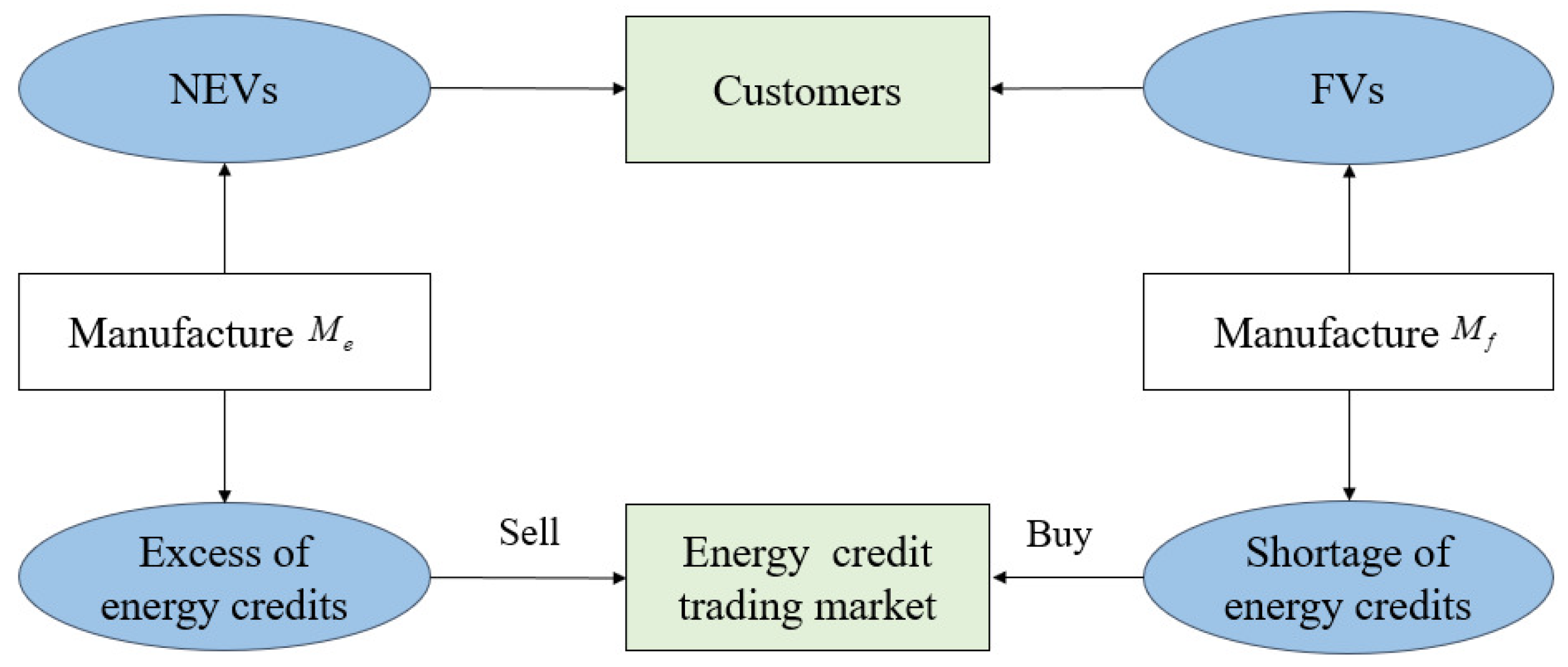
To promote the production of NEVs from the supply side, the social planner introduces a series of measures, such as a ZEV mandate and a dual-credit policy to require manufacturers to achieve the regulation. The dual-credit policy can be regarded as an enhanced version of ZEV mandate, which not only requires a certain quota energy credit to meet the standards but also penalizes unqualified FVs. We assume that the production of NEVs generates positive energy credit and that the production of FVs produces negative energy credits. If the manufacturer cannot clear the negative credits during the year-end accounting, it bears high fines. Without loss of generality, we assume that each NEV generates 1 energy credit and that each FV generates −1 energy credit. Moreover, the social planner specifies the green credit quota (GCQ) for manufacturers, which requires that the energy credit of the NEV to the energy credit of total vehicles is above a certain threshold, denoted as .
Manufacturers can obtain positive energy credit in the following two ways. One is to produce NEVs to generate the required GCQ. If they cannot produce as many as required, they can make up the gap by purchasing energy credits from the energy credit market, where other manufacturers sell extra energy credits. In our model, manufacturer
only produces an NEV, so it can sell all energy credits generated. Manufacturer
only produces FVs and needs to purchase additional energy credit depending on their production strategy. The market structure with energy credit trading system is shown in
Figure 3. For example, “The average fuel consumption of passenger car companies and the new energy vehicle credit management platform” in China provides a market for credit trading for vehicle manufacturers (
http://cafcnev.miit-eidc.org.cn/, (accessed on 21 March 2021)). Thus, in the energy credit trading market, manufacturer
can sell all energy credits generated and manufacturer
needs to purchase energy credits depending on the total production quantity, which is
, where
is the required energy credits and
is to offset the negative energy credit generated by producing FVs. Hence, the problems of the manufacturers are as follows:
Proposition 4. For the production regulation scenario, when GCQ is given, the optimal decision of manufacturers and are as follows:
- (1)
if , manufacturer quits the market and manufacturer posts the optimal price ;
- (2)
if , manufacturer quits the market and manufacturer posts the optimal price ;
- (3)
if , both manufacturers exist in the market, then
;
- (4)
if , manufacturer quits the market and manufacturer posts the optimal price ; and
- (5)
if , manufacturer quits the market and manufacturer posts the optimal price ,
where , , .
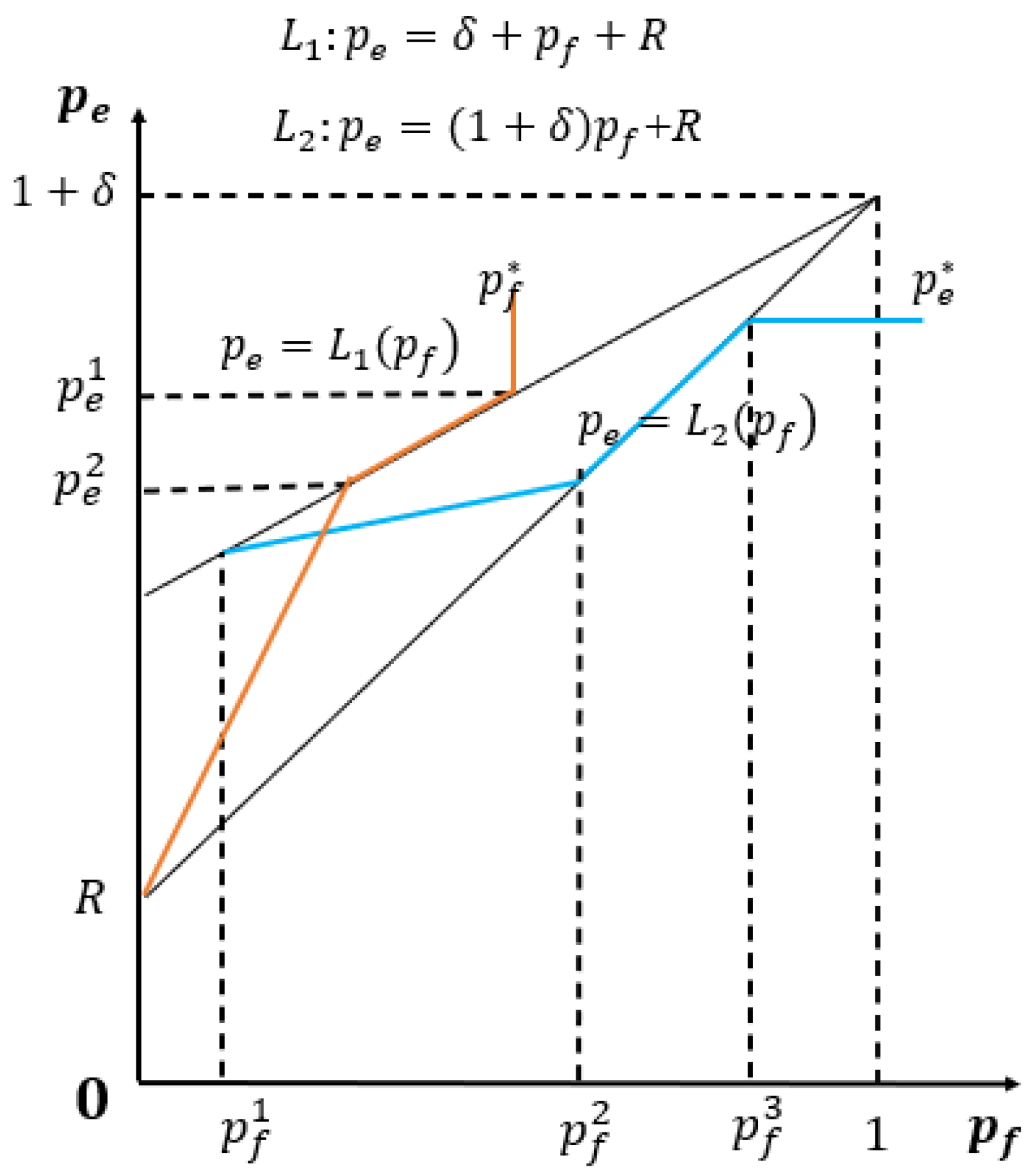
Under the production regulation scheme, the equilibrium prices depend on the GCQ
set by the social planner. We provide some explanation based on
. In the early stage of policy implementation, when the GCQ is relatively small, i.e.,
, manufacturer
does not have enough incentive to enter the market. Manufacturer
dominates the market and posts the price
. Compared with the basic scenario, manufacturer
purchases the energy credit and transfers this cost to consumers, which indicates a higher retail price, i.e.,
. Due to the monopoly of manufacturer
, consumers have no choice but to pay a higher price than before if they want to purchase a FV. When the GCQ becomes larger, i.e.,
, manufacturer
has the possibility to enter the market subject to policy incentives. Manufacturer
chooses to set lower prices
to resist the NEV entering the market, which increases the quantity of the FV. As the policy is further tightened, manufacturer
enters the market and competes with manufacturer
, who sets a higher price (
) to share the market with manufacturer
. When
, the marginal benefit of manufacturer
to produce an FV is less than 0, i.e.,
. Manufacturer
posts the price
and drives manufacturer
out of the market. Finally, if
, manufacturer
has monopolized the market and is not subject to production regulation scheme. Therefore, they set a higher price than before to fully extract consumer surplus. The equilibrium price, quantity, and profit of manufacturers are shown in
Table 8 and
Table 9.
Proposition 5. When NEVs and FVs both exist in the market, i.e., ,
the optimal price, quantity of the NEVs both increases with GCQ, Thus, the profit of manufacturer increases with incentive, i.e., , , ;
the optimal price of the FVs increase with the GCQ, while the quantity of FVs and the profit of manufacturer both decrease with incentive, i.e., , , ; and
the total quantity of vehicles in the market is lower than that of basic scenario, i.e., .
Proposition 5 shows that, when NEVs and FVs both exist in the market, manufacturer produces more NEVs and manufacturer produces less FVs with higher GCQ, which is consistent with our intuition. The increase of GCQ requires manufacturer to purchase more energy credits. Manufacturer increases the retail price to cover the cost due to energy credits. Then, we can obtain that the profit of manufacturer decreases with the GCQ while the profit of manufacturer increases. Furthermore, the impact of the production regulation on the total vehicles is negative. From , we know that the growth rate of NEVs is less than the decline rate of FVs.
Recall proposition 3 in which the demand subsidy stimulates the overall sales of vehicles whereas production regulation reduces the total number of vehicles in the market. This result provides an explanation for the decrease in overall sales in the vehicle market after China implemented the dual-credit policy in 2018. The overall sales of NEVs were 1.25 million in 2018, which was 110% higher than that in 2017. However, the total sales of the vehicle market were 28.08 million, which decreased by 2.8% compared to that in 2017. The implementation of dual-credit policy promotes the growth of NEVs but suppresses the development of FVs effectively, thereby reducing overall sales.
4. The Social Planner Decisions
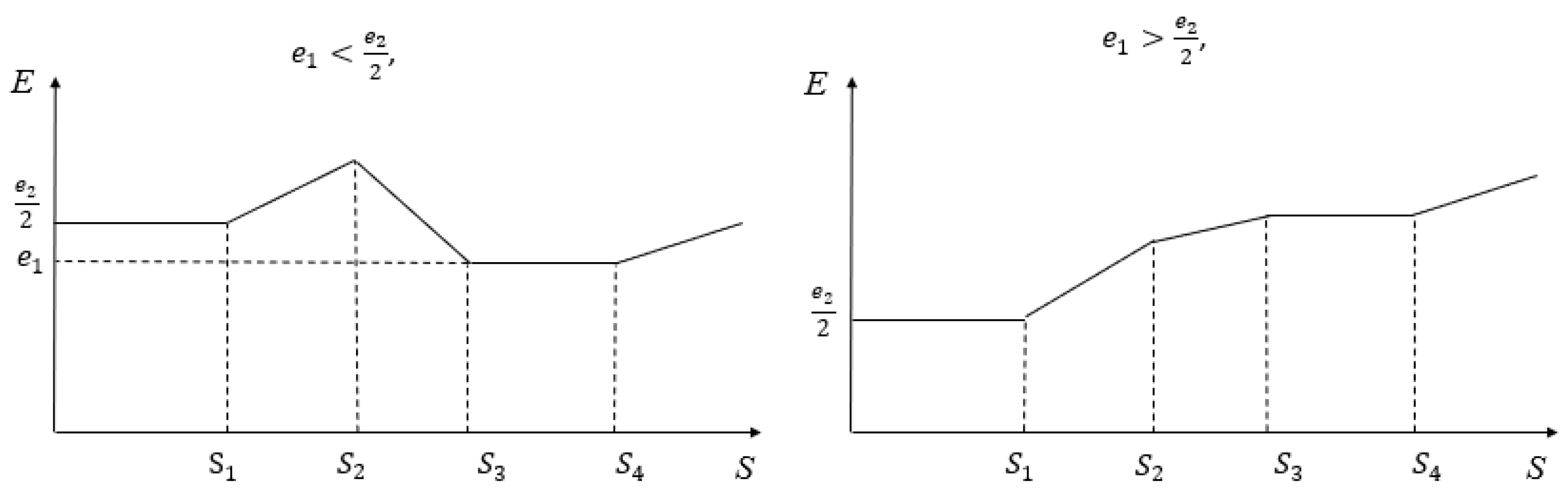
Recall that the main purpose of promoting NEVs is to improve the environment. We first explore the effects of two types of policies on the environment impact. Denote the unit environmental impact of the NEV and the FV as and , respectively. The total environmental impact of the vehicle market can be computed as , where and represent the total environmental impacts of the NEVs and the FVs. Since the impact of vehicles on the environment is generally harmful, we assume that the environmental impact of vehicles is better smaller.
Proposition 6. Compared with no policy intervention, production regulation always reduces environmental impact, i.e., . However, demand subsidy may increase environmental impact, depending on the environmental attributes of NEVs, i.e., if and , otherwise, .
Proposition 6 reveals the effect of two types of policies on environmental impact. Production regulation not only increases the quantity of NEVs but also cuts down the total amount of vehicles, thereby reducing the environmental impact. However, demand subsidy always increases the total amount of vehicles. Therefore, only when the NEVs are very environmentally friendly () does demand subsidy benefit the environment.
Then, to investigate how the social planner decides on the optimal subsidy or the GCQ with the goal of maximizing social welfare, we assume that there is an upper bound for environmental impact, which is an exogenous parameter in the following model. For nontrivial analysis, we assume . The social welfare consists of the manufacturers’ total profits, the consumer surplus, the social planner expenditure, or the profit of energy credit trading market.
Consumer surplus (CS) is defined as the aggregate utility of consumers in the vehicle market. Following, the CS in the production regulation scenario can be constructed as follows:
When demand subsidy is adopted, the consumer’s utility function changes; thus, the CS in the demand subsidy scenario is
Thus, the problem of social planner to implement the demand subsidy is shown as follows:
The optimal demand subsidy
of social planner is presented in
Table 10.
Table 10 shows the optimal subsidy selection follows three parameters, including the unit production cost of NEV
, the unit environment impact of the NEV
, and the environment impact upper bound
. We divided equilibrium into four cases based on the unit NEV production cost
and unit NEV environmental impact
: (1) high cost and low environmentally friendly, i.e.,
, which indicates that adopting high cost produces a low environmentally friendly NEV; (2) high cost and high environmentally friendly:
, which represents that adopting high cost produces a high environmentally friendly NEV; (3) low cost and low environmentally friendly:
; and (4) low cost and high environmentally friendly:
.
Proposition 7. From Table 10, we have following result: in cases 1 and 3, the optimal subsidy decreases in , i.e., ;
in cases 2 and 4, the optimal subsidy increases in with , i.e., ; and
when is large enough, i.e., , the optimal subsidy is , which is independent of .
We observe that, in cases 1 and 3, the optimal subsidy decreases with , i.e., small induces large . In this case, the NEV is very environmentally friendly (), so when the environmental impact upper bound is small (), increased subsidy promotes the production of NEVs, regardless of whether the production cost is high or low. Second, in cases 2 and 4, the optimal subsidy increases with , i.e., small induces small . This reason is as follows. Recall Proposition 1 that the rising subsidy leads to an increase in overall quantity of vehicles. As the unit environment impact of the NEV is low environmentally friendly (), increased subsidy cannot improve the environment. Last, when the environmental impact upper bound is large enough, the amount of subsidy is independent on , which is common in four cases.
Next, we study the social planner’s optimal decisions of GCQ under a production regulation scenario. The problem in model R is shown as follows:
The optimal GCQ decision
of social planner is presented in
Table 11.
Proposition 8. From Table 11, we have following result: when is relatively small, the optimal GCQ τ decreases with , i.e., if ;
production regulation cannot always improve social welfare.
When adopting production regulation policies, we find that the optimal decision on is independent of the unit environment impact of the NEV , which is different from the optimal decision of demand subsidy policy. First, we observe that, when is small, the optimal GCQ decreases with , i.e., small results in large . which indicates that the stricter the environmental impact constraints, the higher the value of GCQ. The reason is that the increase in GCQ always decreases the total number of vehicles, which leads to a positive environmental impact. Recall that the implementation of production regulation policies does have a positive impact on the environment. However, proposition 8 indicates that production regulation cannot always improve social welfare. When the environmental impact upper bound is large, we find that not implementing GCQ maximizes social welfare, i.e., . This is because the positive impact of the implementation of GCQ on the environment cannot offset the negative impact of the decline in manufacturers’ profit and consumer surplus.
In summary, demand subsidy can change the environmental impact positively or negatively, depending on the environmental properties of the NEVs, but it improves social welfare. Production regulation has a positive impact on the environment, but this result comes at the expense of social welfare.
5. Numerical Analysis
In this section, we compare the trend of social welfare with environmental impact upper bound
under two types of policies. Due to the complexity of equilibrium, we show the results with numerical examples. Recall that
and
are the social welfare under demand subsidy and production regulation scenario, respectively. Based on the survey report in China Association of Automobile Manufacturers (
http://www.caam.org.cn/chn/21.html, (accessed on 21 March 2021)), we obtain the parameters as follows:
,
g/mile, and
g/mile. Without loss of generality, we normalized the parameters to values in [0,1].
The dashed line (
) parallel to the x-axis in the
Figure 4 represents the value of social welfare without social planner . From
Figure 4, we observe that production regulation better controlling the environmental impact of vehicles than demand subsidy. For example, if the environmental impact upper bound is large (
), there is
with the same
. Demand subsidy now dominates over production regulation, controlling the environmental impact with
while obtaining more social welfare than production regulation. In summary, production regulation can achieve stricter environmental impact limits but at the expense of social welfare. Demand subsidy is preferred when restrictions are looser, while performing ineffective if
is small. Then, when could the production regulation dominate?
Figure 5 shows the optimal social welfare with the change in
. The only difference between the parameters used in
Figure 4 and
Figure 5 is
, which changes from
to
. We can see that there is an interval such that, given the same
, the social welfare under production regulation is larger than that of demand subsidy, i.e.,
. Therefore, when consumers have a higher preference for NEVs, production regulation is preferred.
6. Conclusions
NEVs, a new type of green vehicle, has received global attention due to the energy crisis and environmental pollution caused by global automobiles. Countries have implemented various policies related to demand subsidy and production regulation to promote the development of NEVs. In this paper, we constructed three competitive environments for FV and NEV manufacturers, namely, without social planner intervention, with demand subsidy, and with production regulation. Based on game models, we derived the manufacture’s optimal price and quantity under three scenarios. Considering social welfare and environmental impact, the social planner’s decision on subsidy and GCQ are also obtained. The main findings are as follows.
Economically, without social planner intervention, only when the production cost of NEVs is low enough can NEVs enter the market and compete with FVs. The social planner’s policy to promote the development of NEVs can offset the disadvantages of production costs. It turns out that the implementation of the two types of policies can effectively increase the quantity of NEVs. However, the impact of the two types of policies on the structure of the vehicle market is different. Demand subsidy increases the overall number of FVs and NEVs. While the production regulation reduces the total number of vehicles while developing NEVs. This result inspires that we can apply these policies in different scenarios. For regions economically developed and with high car parc, although demand subsidy promotes the development of NEVs, they also increase the total number of vehicles, thus making the traffic load heavier. Therefore, production regulation is an ideal choice. On the contrary, for regions less economically developed and with low car parc, demand subsidy can not only promote the adoptions of NEVs but also increase overall car quantity to boost the economic development, which kills two birds with one stone.
Socially, the optimal social welfare is determined by the environmental impact upper bound, the unit production cost of NEVs , and the environmental attributes of NEVs. Moreover, compared with the benchmark with no policy intervention, demand subsidy policies generally improve social welfare while production regulation improves social welfare only with a high consumer preference for NEVs. Nevertheless, production regulation always has a positive impact on the environment, whereas the impact of demand subsidy policies on the environment depends on the environmental properties of NEVs. Numerical analysis shows that consumer environmental preferences and the regulation of environmental impact determine which type of policy dominates the other. In summary, if social planners pay more attention to improving social welfare, then demand subsidy is the optimal choice. Otherwise, social planners prefer production regulation to more emphasis on improving the environment.


