Estimation of the Optimal Threshold Policy in a Queue with Heterogeneous Servers Using a Heuristic Solution and Artificial Neural Networks

Abstract

This paper deals with heterogeneous queues where servers differ not only in service rates but also in operating costs. The classical optimisation problem in queueing systems with heterogeneous servers consists in the optimal allocation of customers between the servers with the aim to minimise the long-run average costs of the system per unit of time. As it is known, under some assumptions the optimal allocation policy for this system is of threshold type, i.e., the policy depends on the queue length and the state of faster servers. The optimal thresholds can be calculated using a Markov decision process by implementing the policy-iteration algorithm. This algorithm may have certain limitations on obtaining a result for the entire range of system parameter values. However, the available data sets for evaluated optimal threshold levels and values of system parameters can be used to provide estimations for optimal thresholds through artificial neural networks. The obtained results are accompanied by a simple heuristic solution. Numerical examples illustrate the quality of estimations.

1. Introduction

Many queueing systems are analysed for their dynamic and optimal control related to system access, resource allocation, changing service area characteristics and so on. Sets of computerised tools and procedures provide large data sets which can be useful to expand potential of classical optimisation methods. The paper deals with a known model of a multi-server queueing system with controllable allocation of customers between heterogeneous servers which are differentiated by their service and cost attributes. For the queueing system with two heterogeneous servers it has been shown in [1] by using a dynamic programming approach that to minimise the mean sojourn time of customers in the system, the faster server must be always used and the customer has to be assigned to the slower server if and only if the number of customers in the queue exceeds the certain threshold level. Furthermore, this result was obtained independently in more simple form in [2,3]. In [4], the author has analysed a multi-server version of such a system and confirmed a threshold nature of the optimal policy as well.

The problem of an optimal allocation of customers between heterogeneous servers in queueing systems with additional costs with the aim to minimise the long-run average cost per unit of time is notoriously more difficult. Some progress has been made after the appearance of a review paper [5]. In [6,7], the authors studied a model with set-up costs using a hysteretic control rule, thereby stressing the algorithmic aspects of the optimal control structure. The same system has been discussed in [8], where a direct method that provides a closed-form expression for the stationary occupancy distribution was proposed. In [9,10], the authors have used theoretical study and exhaustive numerical analysis to show that for some specified servers, ordering the optimal allocation policy which minimises the long-run average cost belongs to a set of structural policies. In other words, for the servers’ enumeration (1), the allocation control policy denoted by f can be defined through a sequence of threshold levels $1=q_1\le q_2\le \cdots \le q_K<\infty$. With respect to the defined policy, the server operating at highest rate should remain busy by non-empty queueing system. The kth server ($k\ge 2$) is used only if the first $k-1$ servers are busy and the queue length reaches a threshold level $q_k>0$. In the general case, the optimal threshold levels can depend on states of slower server and formally the optimal policy f is not of a pure threshold type. However, since the kth threshold value may vary by at most one when the state of slower server changes and it has a weak effect on the average cost, such influence can be neglected. Hence the optimal allocation policy for multi-server heterogeneous queueing system can be treated as a threshold one.

Searching for the optimal values of $q_2,\cdots ,q_K$ by direct minimising the average cost function can be expensive, especially when K is large. To calculate the optimal threshold levels we can use a policy-iteration algorithm [11,12,13] which constructs a sequence of improved policies that converges to optimal one. This algorithm is a fairly versatile tool for solving various optimisation problems. Unfortunately, as is usually the case in practice, this algorithm is not without some limitations, such as the difficulties associated with convergence when the traffic is close to loaded, limitation on the process dimension and, consequently, on the number of states. Thus, we would like to compensate for some of the weaknesses of this algorithm with other methods for calculating the optimal control policy. The contribution of this paper can be briefly described in two conceptual parts. In the first part, we propose a heuristic solution (HS) to obtain functional relationships for optimal thresholds based on a simple discrete approximation of the system’s behaviour. The second part is devoted to the alternative machine learning technique such as artificial neural networks (NN) [14,15,16] which is used again for the estimation of the optimal threshold levels. The policy-iteration algorithm is used in the paper to generate the data sets needed both to verify the quality of the proposed optimal threshold estimation methods and to train the neural networks. We strongly believe that the trained neural network can be successfully used to calculate the optimal thresholds for those system parameters for which alternative numerical methods are difficult or impossible to use, for example, in heavy traffic case, or, in general, to reconstruct the areas of optimality without usage of time-expensive algorithms and procedures. There are some number of papers on prediction of the stochastic behaviour of queueing systems and networks using machine learning algorithms, see e.g., [17,18] and references therein. However, we unsuccessfully tried to find published works where heuristics and machine learning methods would be used to solve a similar optimisation problem for heterogeneous queueing systems and therefore we consider this paper relevant.

This paper is organised as follows. In Section 2, we briefly discuss a mathematical model. Section 3 introduces some heuristic choices for threshold levels that turn out to be nearly optimal. Section 4 presents results when the trained neural network was ran on verification data of the policy-iteration algorithm.

2. Mathematical Model

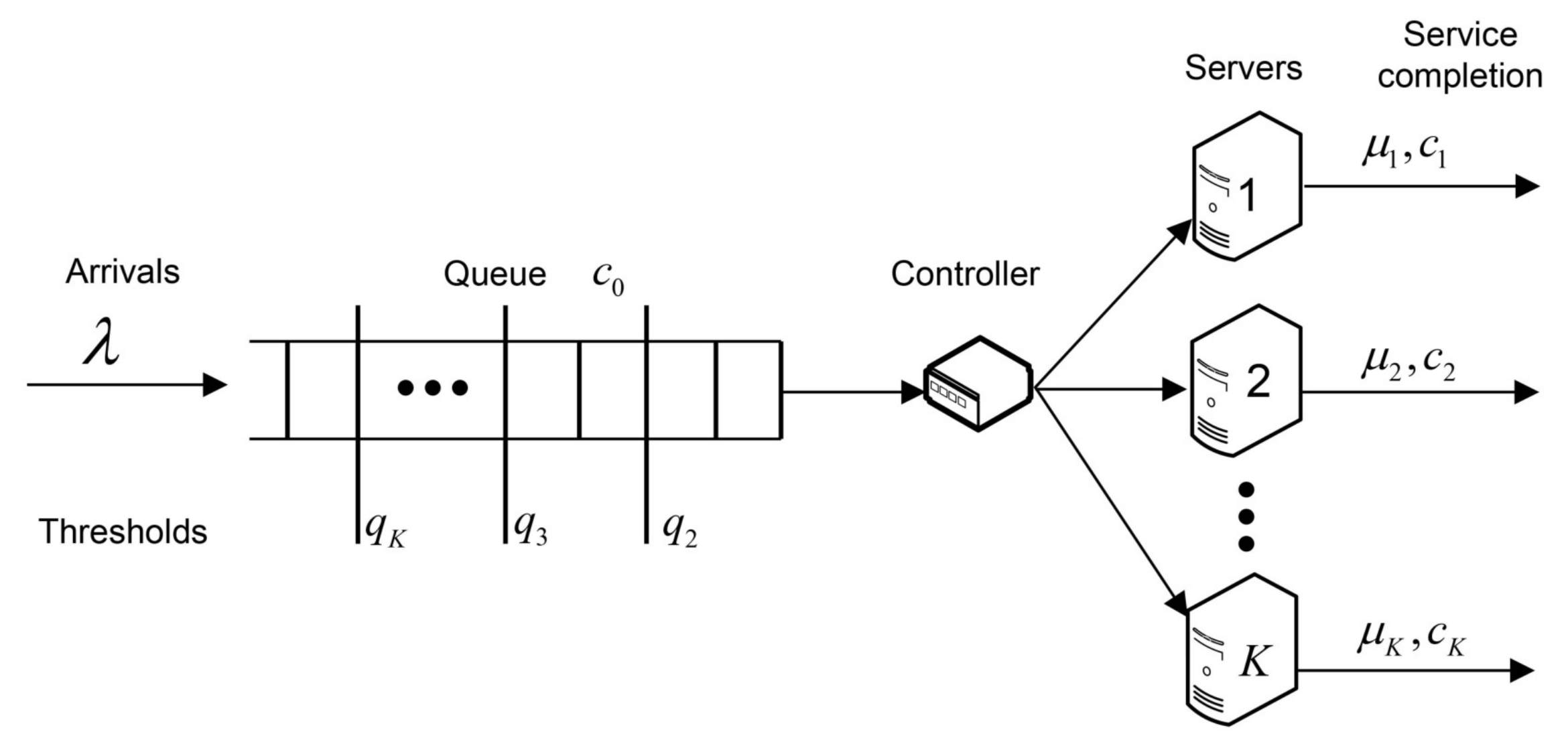
We summarise briefly the model under study. The queueing system is of the type $M/M/K$ with infinite-capacity buffer and K heterogeneous servers. This system is shown schematically in Figure 1. The Poisson arrival stream has a rate $\lambda$ and the exponential distribution of the service time at server j has a rate ${\mu }_j$. We assume that the service in the system is without preemption, when customer in service cannot change the server. The random variables of the inter-arrival times and the service times of the servers are assumed to be independent. An additional cost structure is introduced, consisting of the operating cost $c_j>0$ per unit of time of service on server j and the holding cost $c_0>0$ of waiting in the queue. Assume that the servers are enumerated in a way   

$$\begin{array}{c}\hfill {\mu }_1\ge \cdots \ge {\mu }_K,c_1{\mu }_1^{-1}\le \cdots \le c_K{\mu }_K^{-1},\end{array}$$

(1)

where $c_j{\mu }_j^{-1}$ stands for the mean operating cost per customer for the jth server.

Figure 1. Controllable multi-server queueing system with heterogeneous servers and operating costs.

The controller has full information about the system’s state and, based on this information, can make control actions on the system at the decision epochs when certain state transitions occur, following the prescription of the policy f. In our case, the controller selects the control action at the time when a new customer enters the system and at the service completion times, if the queue is not empty. When a new customer arrives, it joins the queue and at the same time, the controller sends another customer from the head of the queue to one of the idle servers or leaves it in the queue. At the service completion, the customer leaves the corresponding server, and at the same time the controller takes the next customer from the head of the queue, if it is not empty, and dispatches it to one of idle servers or can leave it in the queue as well. The service completion in the system without waiting customers does not require the controller to perform any control action.

The fact that the optimal policy for the problem of minimising the long-run average cost per unit of time belongs to a set of threshold-based policies for the multi-server heterogeneous queueing systems with costs were proved first in [10] and further conformed for systems with heterogeneous groups of servers in [19]. The corresponding optimal thresholds can in the general case depend on the states of slower servers. However, according to obtained numerical results in [9], we can neglect the weak influence of the slower servers’ states on the optimal allocation policy for the faster servers. This phenomena was discussed additionally in Example 2. Therefore, we may assume that the optimal policy belongs to the class of a pure threshold policy when the use of a certain server depends solely on the number of waiting customers in the queue. Specifically, for the system under study, such a policy is defined by the following sequence of threshold levels:

$$\begin{array}{c}\hfill 1=q_1\le q_2\le \cdots \le q_K<\infty .\end{array}$$

(2)

The policy prescribes the use of the k fastest servers whenever the number of customers waiting in the queue satisfies the condition $q_k\le q\le q_{k+1}-1$.

To calculate optimal thresholds we need to formulate the introduced optimisation problem in terms of a Markov decision process. This process is based on a $K+1$-dimensional continuous-time Markov chain

$${\left\{X\left(t\right)\right\}}_{t\ge 0}={\{Q\left(t\right),D_1\left(t\right),\cdots ,D_K\left(t\right)\}}_{t\ge 0}$$

(3)

with an infinitesimal matrix ${\Lambda }^f$ which depends on the policy f. Here the component $Q\left(t\right)\in {\mathbb{N}}_0$ stands for the number of waiting customers at time t and

$$D_j\left(t\right)=\left\{\begin{array}{cc}0\hfill & \mathrm{if}j\mathrm{th}\mathrm{server}\mathrm{is}\mathrm{idle}\hfill \\ 1\hfill & \mathrm{if}j\mathrm{th}\mathrm{server}\mathrm{is}\mathrm{busy}\hfill \end{array}\right..$$

The state space of the process ${\left\{X\left(t\right)\right\}}_{t\ge 0}$ operating under some policy f is $E^f=\{x=(q\left(x\right),d_1\left(x\right),\cdots ,d_K\left(x\right))\}\subseteq {\mathbb{N}}_0\times {\{0,1\}}^K$, where the notations $q\left(x\right)$ and $d_j\left(x\right)$ are used respectively for the queue length and for the state of jth server in state $x\in E^f$.

The possible server states are partitioned as follows:

$$J_0\left(x\right)=\{j:d_j\left(x\right)=0\},J_1\left(x\right)=\{j:d_j\left(x\right)=1\}.$$

The sets $J_0\left(x\right)$ and $J_1\left(x\right)$ denote the sets of idle and busy servers in state $x\in E^f$, respectively. The set of control actions a is $A=\{0,1,\cdots ,K\}$. If $a=0$, the controller allocates a customer to the queue. Otherwise, if $a\ne 0$, the controller instructs a customer to occupy the server with a number a. In addition, we can define the subsets $A\left(x\right)=J_0\left(x\right)\cup \left\{0\right\}\subseteq A$ of admissible actions in state x The policy f specifies the choice of a control action at any decision epoch and the infinitesimal matrix ${\Lambda }^f=\left[{\lambda }_{xy}\left(a\right)\right]$ of the Markov-chain (3) has then the following elements,

$$\begin{array}{c}\hfill {\lambda }_{xy}\left(a\right)=\left\{\begin{array}{cc}\lambda \hfill & y=x+{\mathbf{e}}_a,j\in A\left(x\right)\hfill \\ {\mu }_j\hfill & y=x-{\mathbf{e}}_j,j\in J_1\left(x\right),q\left(x\right)=0\hfill \\ {\mu }_j\hfill & y=x-{\mathbf{e}}_j-{\mathbf{e}}_0+{\mathbf{e}}_a,a\in A(x-{\mathbf{e}}_j-{\mathbf{e}}_0),q\left(x\right)>0,\hfill \end{array}\right.\end{array}$$

where ${\mathbf{e}}_j$ is defined as $K+1$-dimensional unit vector with each element equal to zero except the jth position ($j=0,1,\cdots ,K$).

We will search for the optimal control policy among the set of stationary Markov policies f that guarantee ergodicity of the Markov chain ${\left\{X\left(t\right)\right\}}_{t\ge 0}$. The corresponding stability condition is obviously defined as $\lambda <{\sum }_{j=1}^K{\mu }_j$. It follows from the fact, that if number of customers exceeds a threshold $q_K$, then the queueing systems behaves like a $M/M/1$ queue with an arrival rate $\lambda$ and total service rate ${\mu }_1+\cdots +{\mu }_K$. As it is known, see e.g., [13], the ergodic Markov chain with costs implies the equality of the long-run average cost per unit of time for the policy f and the corresponding assemble average, that can be written in the form

$$\begin{array}{c}\hfill g^f=\underset{t\to \infty }{lim\; sup}\frac{1}{t}{V}^f(x,t)=\sum _{y\in E^f}c\left(y\right){\pi }_y^f,\end{array}$$

(4)

where $c\left(y\right)=c_{0}q\left(y\right)+{\sum }_{j=1}^K{c}_j{d}_j\left(y\right)$ is an immediate cost in state $y\in E^f$. The cost function $V^f(x,t)$ is given by

$$\begin{array}{c}\hfill V^f(x,t)={\mathbb{E}}^f\left[{\int }_0^t\left(c_{0}Q\left(t\right)+\sum _{j=1}^K{c}_j{D}_j\left(t\right)\right)dt|X\left(0\right)=x\right].\end{array}$$

This function describes the total average cost up to time t given the initial state is x and ${\pi }_y^f={\mathbb{P}}^f[X\left(t\right)=y]$ is a stationary state distribution for the policy f. The policy $f^{*}$ is said to be optimal when for $g^f$ defined in (4) we evaluate

$$\begin{array}{c}\hfill g^{*}=\underset{f}{inf}{g}^f=\underset{q_2,\cdots ,q_K}{min}g(q_2,\cdots ,q_K).\end{array}$$

(5)

To evaluate optimal threshold levels and optimised value for the mean average cost per unit of time the policy-iteration Algorithm 1 is used. This algorithm constructs a sequence of improved policies until the average cost optimal is reached. It consists of three main steps: value evaluation, policy improvement and threshold evaluation. The Value evaluation is based on solving, for a given policy f, a system of linear equations

$$\begin{array}{c}\hfill v^f\left(x\right)=\frac{1}{{\lambda }_x\left(a\right)}\left(c\left(x\right)+\sum _{y\ne x}{\lambda }_{xy}\left(a\right)v^f\left(y\right)-g^f\right).\end{array}$$

(6)

Algorithm 1 Policy-iteration algorithm

1: procedurePIA($K,W,\lambda ,{\mu }_j,c_j,j=1,2,\cdots ,K,c_0$) 2:     $f^{\left(0\right)}\left(x\right)={argmin}_{j\in J_0\left(x\right)}\left\{\frac{c_j}{{\mu }_j}\right\}$                              ▹ Initial policy 3:     $n\leftarrow 0$ 4:     $g^{f^{\left(n\right)}}=\lambda v^{f^{\left(n\right)}}\left({\mathbf{e}}_1\right)$                                  ▹ Value evaluation 5:     for $x=(0,1,0,\cdots ,0) \mathbf{to} (N,1,1,\cdots ,1)$ do 6:          $$\begin{array}{cc}\hfill v^{f^{\left(n\right)}}\left(x\right)& =\frac{1}{\lambda +{\sum }_{j\in J_1\left(x\right)}{\mu }_j}[c\left(x\right)-g^{f^{\left(n\right)}}+\lambda v^{f^{\left(n\right)}}(x+{\mathbf{e}}_{f^{\left(n\right)}\left(x\right)})\hfill \\ & +{\displaystyle \sum _{j\in J_1\left(x\right)}}{\mu }_j{v}^{f^{\left(n\right)}}(x-{\mathbf{e}}_j)1_{\left\{q\right(x)=0\}}\hfill \\ & +{\displaystyle \sum _{j\in J_1\left(x\right)}}{\mu }_j{v}^{f^{\left(n\right)}}(x-{\mathbf{e}}_j-{\mathbf{e}}_0+{\mathbf{e}}_{f^{\left(n\right)}(x-{\mathbf{e}}_j-{\mathbf{e}}_0)})1_{\left\{q\right(x)>0\}}]\hfill \end{array}$$ 7:     end for 8:                                   ▹ Policy improvement $$f^{(n+1)}\left(x\right)={argmin}_{a\in A\left(x\right)}{v}^{f^{\left(n\right)}}(x+{\mathbf{e}}_a)$$ 9:     if $f^{(n+1)}\left(x\right)=f^{\left(n\right)}\left(x\right),x\in E^f$ then return $f^{(n+1)}\left(x\right),v^{f^{\left(n\right)}}\left(x\right),g^{f^{\left(n\right)}}$ 10:     else  $n\leftarrow n+1$, go to step 4 11:     end if 12:                                   ▹ Threshold evaluation $$q_k:f^{(n+1)}(q,1,\cdots ,1,0,d_{k+1},\cdots ,d_K)=\left\{\begin{array}{cc}0\hfill & q\le q_k-2\hfill \\ k\hfill & q>q_k-2\hfill \end{array}\right.,k=2,\cdots ,K$$ 13: end procedure

For the dynamic-programming value function $v^f:E^f\to \mathbb{R}$, which indicates a transition effect of an initial state x to the total average cost and satisfies the following asymptotic relation,

$$V^f(x,t)=g^{f}t+v^f\left(x\right)+o\left(1\right),t\to \infty ,x\in E^f.$$

In order to make the system (6) solvable, one of the values $v\left(x\right)$ must be set to zero, e.g., for $x_0=(0,\cdots ,0)$ we set $v\left(x_0\right)=0$. Since in our case $c\left(x_0\right)=0$, the first equation of the system (6) is of the form $g^f={\sum }_{y\ne x_0}{\lambda }_{x_{0}y}\left(a\right)v^f\left(y\right)$. In the policy improvement step a new policy $f^{\prime }$ is calculated by minimising the value function $v(x+{\mathbf{e}}_a)$ for any state $x\in E^f$ and any admissible control action $a\in A\left(x\right)$. The algorithm converges if the policies f and $f^{\prime }$ on neighbouring iterations are equal. In the threshold evaluation we calculate the optimal thresholds $q_k$, $k=2,\cdots ,K$, based on optimal policy f. As an initial policy we select the policy which prescribes in any state the usage of a server j with the minimal value of the mean operating cost $\frac{c_j}{{\mu }_j}$ per customer. More detailed information on deriving the dynamic programming equations for the heterogeneous queueing system and calculating the corresponding optimal allocation control policy can be found in [9]. For existence of an optimal stationary policy and convergence of the policy-iteration algorithm we refer to [12,20,21,22].

To realise the policy-iteration algorithm we convert the $K+1$-dimensional state space $E^f$ of the Markov decision process to a one-dimensional equivalent state space. Let $\Delta :E^f\to {\mathbb{N}}_0$ be a one-to-one mapping of the vector state $x=(q\left(x\right),d_1\left(x\right),\cdots ,d_K\left(x\right))\in E^f$ to a value from ${\mathbb{N}}_0$ which is of the form

$$\begin{array}{c}\hfill \Delta \left(x\right)=q\left(x\right)2^K+\sum _{i=1}^K{d}_i\left(x\right)2^{i-1}.\end{array}$$

(7)

A new state after transition involving the addition or removal of customer in some state $x\in E^f$, in a one-dimensional state space is calculated by

$$\begin{array}{cc}\hfill & \Delta (x\pm {\mathbf{e}}_0)=(q\left(x\right)\pm 1)2^K+\sum _{i=1}^K{d}_i\left(x\right)2^{i-1}=\Delta \left(x\right)\pm 2^K,\hfill \\ \hfill & \Delta (x\pm {\mathbf{e}}_j)=q\left(x\right)2^K+\sum _{i=1}^K{d}_i\left(x\right)2^{i-1}\pm 2^{j-1}=\Delta \left(x\right)\pm 2^{j-1}.\hfill \end{array}$$

Further in the algorithm, an infinite buffer system must be approximated by an equivalent system where the number of waiting places is finite but at the same time is sufficiently large. As a truncation criterion, we use the loss probability which should not exceed some small value $\epsilon >0$.

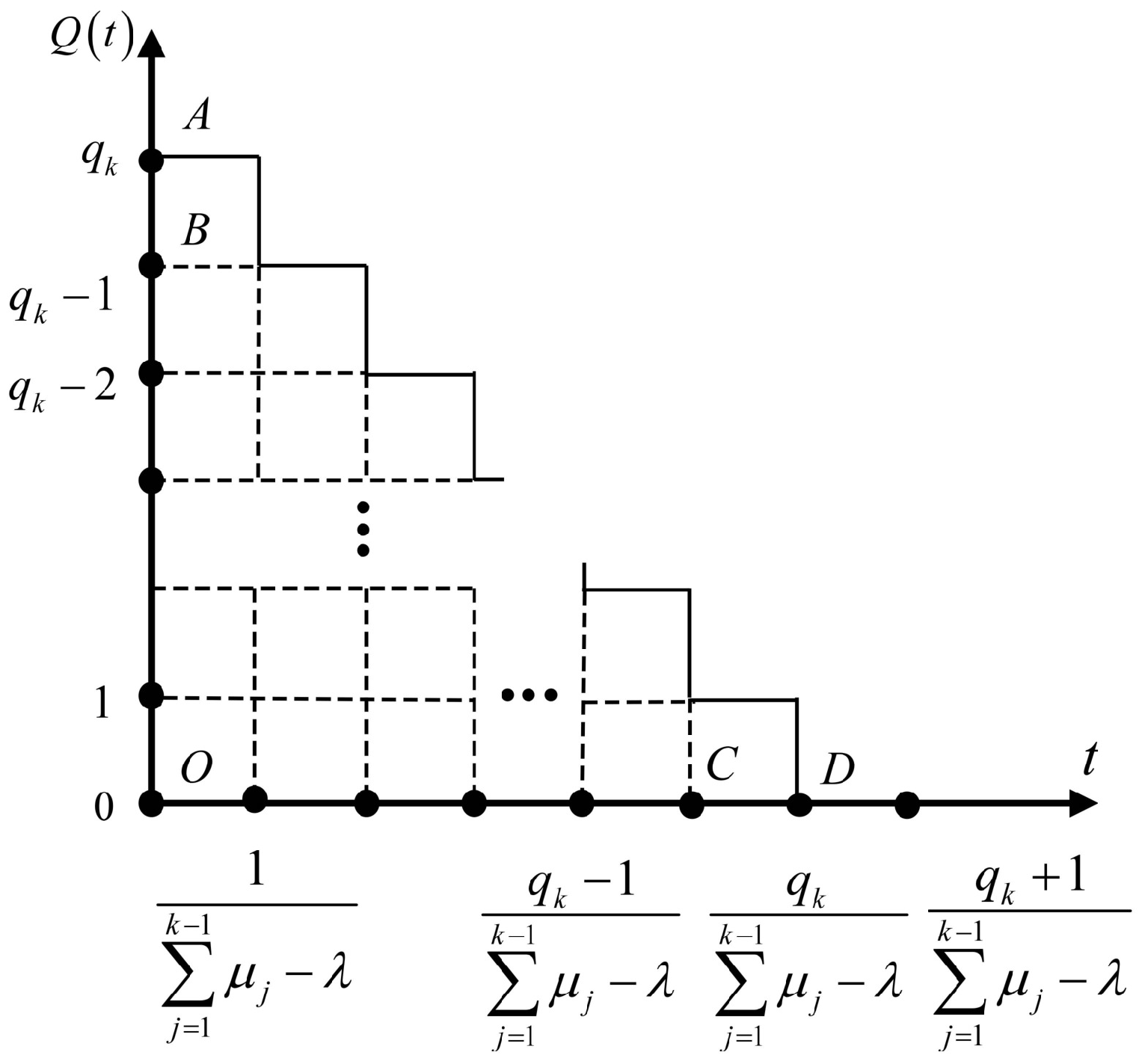
Remark 1.

If the buffer size is W, the number of states is

$$|E^f|=2^K(W+1).$$

In case the number of waiting customers is getting larger as the level $q_K$, all servers must be occupied and the system dynamics is the same as in a classical queue $M/M/1$ with arrival rate λ and service rate ${\sum }_{j=1}^K{\mu }_j$. The stationary state probabilities for the states x where the component $q\left(x\right)\ge q_K$ satisfy the following difference equation

$$\lambda {\pi }_{(q-1,1,\cdots ,1)}-\left(\lambda +\sum _{j=1}^K{\mu }_j\right){\pi }_{(q,1,\cdots ,1)}+\sum _{j=1}^K{\mu }_j{\pi }_{(q+1,1,\cdots ,1)}=0,$$

which has a solution in a geometric form, ${\pi }_{(q,1,\cdots ,1)}={\pi }_{(q_K,1,\cdots ,1)}{\rho }^{q-q_K}$, $q\ge q_K$. For details and theoretical substantiation see, e.g., [23]. Note that the value of $q_K$ included in this formula can be estimated by a heuristic solution (9). Then the truncation parameter W of the buffer size can be evaluated from the following constraint for the loss probability

$$\sum _{q=W}^{\infty }{\pi }_{(q,1,\cdots ,1)}={\pi }_{q_K}\sum _{q=W}^{\infty }{\rho }^{q-q_K}\le \sum _{q=W}^{\infty }{\rho }^{q-q_K}=\frac{{\rho }^{W-q_K}}{1-\rho }<\epsilon ,$$

where $\rho =\frac{\lambda }{{\sum }_{j=1}^K{\mu }_j}$. After simple algebra, it implies

$$W>\frac{log\epsilon (1-\rho )}{log\left(\rho \right)}+q_K.$$

Example 1.

Consider the system $M/M/5$ with $K=5$ and $\lambda =15$. All other parameters take the following values

j	0	1	2	3	4	5
$c_j$	1	5	4	3	2	1
${\mu }_j$	-	20	8	4	3	1
$c_j{\mu }_j^{-1}$	-	0.25	0.50	0.75	0.67	1.00

The truncation parameter W of the buffer size is chosen at value 80 which for $\epsilon =0.0001$ guarantees that $W>\frac{log0.0001(1-14/36)}{log(14/36)}+q_5=22.2734$. Here $q_5=12$ was calculated by (9). In a control table, we summarise the functions $f\left(x\right)$ which specify the control actions at time of arrivals to a certain state x:

System State $\mathit{x}$	Queue Length $\mathit{q}\left(\mathit{x}\right)$
$d=(d_1,d_2,d_3,d_4,d_5)$	0	1	2	3	4	5	6	7	8	9	10	11	12	...
(0,*,*,*,*)	1	1	1	1	1	1	1	1	1	1	1	1	1	1
(1,0,*,*,*)	0	0	2	2	2	2	2	2	2	2	2	2	2	2
(1,1,0,*,*)	0	0	0	3	3	3	3	3	3	3	3	3	3	3
(1,1,1,0,*)	0	0	0	0	4	4	4	4	4	4	4	4	4	4
(1,1,1,1,0)	0	0	0	0	0	0	0	0	0	0	0	5	5	5
(1,1,1,1,1)	0	0	0	0	0	0	0	0	0	0	0	0	0	0

Threshold levels $q_k$, $k=1,\cdots ,K=5$, can be evaluated by comparing the optimal actions $f(q,\underset{k-1}{\underbrace{1,\cdots ,1}},\underset{K-k+1}{\underbrace{0,\cdots ,0}})<f(q+1,\underset{k-1}{\underbrace{1,\cdots ,1}},\underset{K-k+1}{\underbrace{0,\cdots ,0}})$ for $q=0,\cdots ,W-1$. In this example the optimal policy $f^{*}$ is defined here through a sequence of threshold levels $(q_2,q_3,q_4,q_5)=(3,4,5,12)$ and $g^{*}=4.92897$. The bold and underline format in a control table is used to label the change of the control action in a certain system state.

In the next example we give some arguments that allow us to work further only with the threshold-based control policies.

Example 2.

Consider the system $M/M/3$ with $K=3$ servers. The aim of this example consists in the following: With respect to the system states $x=(q,1,0,0)$ and $y=(q,1,0,1)$ the assignment to the second server can in general depend not only on the number of customers in the queue but also on the state of the third server. In this example it is optimal to make an assignment in state x but not in state y. We solve optimisation problem for the following parameters:

• $\lambda =0.238$, ${\mu }_1=0.621$, ${\mu }_2=0.071$ and ${\mu }_3=0.070$,
• $\lambda =0.477$, ${\mu }_1=0.356$, ${\mu }_2=0.096$ and ${\mu }_3=0.070$.

The of optimal solution for the first and second group of system parameters are represented in Table 1 and Table 2, respectively.

Table 1. Control table.

System State x	Queue Length $\mathit{q}\left(\mathit{x}\right)$
$(d_1,d_2,d_3)$	0	1	2	3	4	5	6	7	8	9	10	11	12	13	14	15	16	...
(0,0,0)	1	1	1	1	1	1	1	1	1	1	1	1	1	1	1	1	1	1
(1,0,0)	0	0	0	0	0	2	2	2	2	2	2	2	2	2	2	2	2	2
(0,1,0)	1	1	1	1	1	1	1	1	1	1	1	1	1	1	1	1	1	1
(1,1,0)	0	0	0	0	0	3	3	3	3	3	3	3	3	3	3	3	3	3
(0,0,1)	1	1	1	1	1	1	1	1	1	1	1	1	1	1	1	1	1	1
(1,0,1)	0	0	0	0	2	2	2	2	2	2	2	2	2	2	2	2	2	2
(0,1,1)	1	1	1	1	1	1	1	1	1	1	1	1	1	1	1	1	1	1
(1,1,1)	0	0	0	0	0	0	0	0	0	0	0	0	0	0	0	0	0	0

Table 2. Control table.

System State x	Queue Length $\mathit{q}\left(\mathit{x}\right)$
$(d_1,d_2,d_3)$	0	1	2	3	4	5	6	7	8	9	10	11	12	13	14	15	16	...
(0,0,0)	1	1	1	1	1	1	1	1	1	1	1	1	1	1	1	1	1	1
(1,0,0)	0	2	2	2	2	2	2	2	2	2	2	2	2	2	2	2	2	2
(0,1,0)	1	1	1	1	1	1	1	1	1	1	1	1	1	1	1	1	1	1
(1,1,0)	0	3	3	3	3	3	3	3	3	3	3	3	3	3	3	3	3	3
(0,0,1)	1	1	1	1	1	1	1	1	1	1	1	1	1	1	1	1	1	1
(1,0,1)	2	2	2	2	2	2	2	2	2	2	2	2	2	2	2	2	2	2
(0,1,1)	1	1	1	1	1	1	1	1	1	1	1	1	1	1	1	1	1	1
(1,1,1)	0	0	0	0	0	0	0	0	0	0	0	0	0	0	0	0	0	0

We notice that for most parameter values the optimal decision can be made independently of the states of the slower servers. However, it is interesting to consider the reasons for such possible dependence. It is evident that in our optimisation problem, the optimal policy assigns a customer to the fastest free server in states for which this would not be optimal if there were no arrivals. This is because the system should be ready for possible arrivals, which, if they occur, will wish to see a less congested system.

Consider now the system with three servers in the states $x+{\mathbf{e}}_0+{\mathbf{e}}_1$ and $x+{\mathbf{e}}_1+{\mathbf{e}}_2$, where $x=(0,0,0,0)$. Let us consider the case of potential service completion at the second server, taking into account a large number q of accompanied arrivals. Because of large q, it is optimal to occupy all accessible idle servers. The states mentioned above become $x+(q-1){\mathbf{e}}_0+{\mathbf{e}}_1+{\mathbf{e}}_2+{\mathbf{e}}_3$ and $x+(q-2){\mathbf{e}}_0+{\mathbf{e}}_1+{\mathbf{e}}_2+{\mathbf{e}}_3$. Thus, the difference $v(x+(q-1){\mathbf{e}}_0+{\mathbf{e}}_1+{\mathbf{e}}_2+{\mathbf{e}}_3)-v(x+(q-2){\mathbf{e}}_0+{\mathbf{e}}_1+{\mathbf{e}}_2+{\mathbf{e}}_3)$ of value functions measures the advantage that will be obtained in the case of the assignment to the second processor $x+{\mathbf{e}}_0+{\mathbf{e}}_1\to x+{\mathbf{e}}_1+{\mathbf{e}}_2$. The events of service completion on the second server provide the incentive to make an assignment to the second server. However, if the two initial states are $x+{\mathbf{e}}_0+{\mathbf{e}}_1+{\mathbf{e}}_3$ and $x+{\mathbf{e}}_1+{\mathbf{e}}_2+{\mathbf{e}}_3$, the measure of advantage if service completion takes place is $v(x+q{\mathbf{e}}_0+{\mathbf{e}}_1+{\mathbf{e}}_2+{\mathbf{e}}_3)-v((q-1){\mathbf{e}}_0+{\mathbf{e}}_1+{\mathbf{e}}_2+{\mathbf{e}}_3)$. Since we expect that the value function $v(q{\mathbf{e}}_0+{\mathbf{e}}_1+{\mathbf{e}}_2+{\mathbf{e}}_3)$ is convex in q, it is plausible that the incentive to make an assignment to the second server is greater in state $x+{\mathbf{e}}_0+{\mathbf{e}}_1+{\mathbf{e}}_3$ than in $x+{\mathbf{e}}_0+{\mathbf{e}}_1$. Numerical examples proposed in Table 3 confirm our expectations.

Table 3. Value function for system states.

System State x	Value Function $\mathit{v}\left(\mathit{x}\right)$
$(q,d_1,d_2,d_3)$	example 1	example 2
(0,0,0,0)	0	0
(0,1,0,0)	2.6034	19.4480
(0,0,1,0)	14.0865	28.3810
(0,0,0,1)	14.2872	33.7009
(1,1,0,0)	7.7979	51.3142
(0,1,1,0)	16.6905	51.4444
(0,1,0,1)	16.8910	55.9981
(0,0,1,1)	28.3747	65.9866
(2,1,0,0)	15.5520	96.1454
(1,1,1,0)	21.8874	90.3521
(1,1,0,1)	22.0873	93.2714
(0,1,1,1)	30.9798	93.2581
(3,1,0,0)	25.7823	154.6580
(2,1,1,0)	29.6487	142.7630
(2,1,0,1)	29.8469	145.4230
(1,1,1,1)	36.1809	140.4050
...	...	-
(6,1,0,0)	68.3382	-
(5,1,1,0)	66.8622	-
(5,1,0,1)	66.9946	-
(4,1,1,1)	66.9830	-
(7,1,0,0)	85.9322	-
(6,1,1,0)	82.9672	-
(6,1,0,1)	83.0730	-
(5,1,1,1)	81.9234	-

The further numerical examples show that the threshold levels have a very weak dependence of slower servers’ states. According to our observations, the optimal threshold may vary by at most 1 when the state of a slower server changes.

The data needed either to verify the heuristic solution or for training and verification of the neural network was generated by a policy-iteration algorithm in form of the list

$$\begin{array}{cc}\hfill S=& \{(\lambda ,{\mu }_1,\cdots ,{\mu }_K,c_0,c_1,\cdots ,c_K)\to (q_2,\cdots ,q_K):\hfill \\ \hfill & \lambda \in [1,45],{\mu }_1,\cdots ,{\mu }_K\in [1,40],c_0\in [1,3],c_1,\cdots ,c_K\in [1,5],\hfill \\ \hfill & \lambda <\sum _{j=1}^K{\mu }_j,{\mu }_1\ge \cdots \ge {\mu }_K,c_1{\mu }_1^{-1}\le \cdots \le c_K{\mu }_K^{-1}\}.\hfill \end{array}$$

(8)

Example 3.

Some elements of the list S for the $M/M/5$ queueing system are

$$\begin{array}{cc}\hfill & (1,20,8,4,2,1,1,1,1,1,1,1)\to (2,5,13,30),(10,20,8,4,2,1,1,1,1,1,1,1)\to (1,4,9,21),\hfill \\ \hfill & (1,20,8,4,2,1,1,5,4,3,2,1)\to (5,12,20,20),(10,20,8,4,2,1,1,5,4,3,2,1)\to (3,8,13,13).\hfill \end{array}$$

3. Heuristic Solution

In this section, we want to obtain a heuristic solution (HS) to calculate the optimal thresholds $q_k$, $k=2,\cdots ,K$ for the arbitrary K in explicit form. For this purpose, we will use a simple deterministic approximation for the dynamic behaviour of the number of customers in the queue as illustrated in Figure 2.

Figure 2. Queue length approximation.

Let $q_k$ is an optimal threshold used to dispatch the customer to server k in state $(q_k-1,\underset{k-1}{\underbrace{1,\cdots ,1}},\underset{K-k+1}{\underbrace{0,\cdots ,0}})$, where the first $k-1$ servers are busy. Now we compare the queues of the system given initial state is $x_0=(q_k,\underset{k-1}{\underbrace{1,\cdots ,1}},0,\underset{K-k}{\underbrace{0,\cdots ,0}})$, where the kth server is not used for a new customer, and $y_0=(q_k-1,\underset{k-1}{\underbrace{1,\cdots ,1}},1,\underset{K-k}{\underbrace{0,\cdots ,0}})$, where the kth server is occupied by a waiting customer. It is assumed that the stability condition holds. The initial queue lengths are labelled in Figure 2 by $A=q_k$ and $B=q_k-1$. The proposed deterministic approximation is based on an assumption that the queue length of the system with the first $k-1$ busy servers decreases with the rate ${\sum }_{j=1}^{k-1}{\mu }_j-\lambda$. When this rate is keeping until the queue is empty, it occurs at time points $D=\frac{q_k}{{\sum }_{j=1}^{k-1}{\mu }_j-\lambda }$ and $C=\frac{q_k-1}{{\sum }_{j=1}^{k-1}{\mu }_j-\lambda }$ respectively for the given initial queue length A and B. The total (accumulated) holding times of all customers in the queue with lengths $q_k$ and $q_k-1$ are equal respectively to the number of square blocks of dimension $1\times \frac{1}{{\sum }_{j=1}^{k-1}{\mu }_j-\lambda }$ within the areas $AOD$ and $BOC$ multiplied by the mean service time of the approximated model:

$$\begin{array}{cc}\hfill & F_{AOD}=(q_k+(q_k-1)+(q_k-2)+\cdots +1)\frac{1}{{\sum }_{j=1}^{k-1}{\mu }_j-\lambda }=\frac{q_k(q_k+1)}{2}·\frac{1}{{\sum }_{j=1}^{k-1}{\mu }_j-\lambda }\mathrm{and}\hfill \\ \hfill & F_{BOC}=((q_k-1)+(q_k-2)+\cdots +1)\frac{1}{{\sum }_{j=1}^{k-1}{\mu }_j-\lambda }=\frac{q_k(q_k-1)}{2}·\frac{1}{{\sum }_{j=1}^{k-1}{\mu }_j-\lambda }.\hfill \end{array}$$

The mean operating cost of the first $k-1$ servers during the time period until the queue becomes empty given the initial state is $x_0$ can be calculated by

$$q_k\left(\frac{c_1}{{\mu }_1}\frac{{\mu }_1}{{\sum }_{j=1}^{k-1}{\mu }_j}+\cdots +\frac{c_{k-1}}{{\mu }_{k-1}}\frac{{\mu }_{k-1}}{{\sum }_{j=1}^{k-1}{\mu }_j}\right)=q_k\frac{{\sum }_{j=1}^{k-1}{c}_j}{{\sum }_{j=1}^{k-1}{\mu }_j}.$$

The expression $\frac{{\mu }_i}{{\sum }_{j=1}^{k-1}{\mu }_j}$ means the probability of the service completion at the ith server, and the mean operating cost given the initial state is $y_0$, which can be defined as $(q_k-1)\frac{{\sum }_{j=1}^{k-1}{c}_j}{{\sum }_{j=1}^{k-1}{\mu }_j}$.

Now using the deterministic approximation we can formulate the following proposition.

Proposition 1.

The optimal thresholds $q_k$, $k=2,\cdots ,K$, are defined by

$$\begin{array}{c}\hfill q_k\approx {\widehat{q}}_k=min\left\{1,⌊\frac{{\sum }_{j=1}^{k-1}{\mu }_j-\lambda }{c_0}\left[\frac{c_k}{{\mu }_k}-\frac{{\sum }_{j=1}^{k-1}{c}_j}{{\sum }_{j=1}^{k-1}{\mu }_j}\right]⌋\right\}.\end{array}$$

(9)

Proof. 

Let $V\left(x\right)$ be the overall average system cost until the system becomes empty given the initial state is $x\in E^f$. This value can be represented as a sum of the total holding cost of customers waiting in the queue and mean operating cost of all servers which remain busy in state x. Assume that the controller performs a decision to allocate the customer to the kth server in state $(q_k-1,\underset{k-1}{\underbrace{1,\cdots ,1}},\underset{K-k+1}{\underbrace{0,\cdots ,0}})$. As a result, it leads to a reduction of the overall system costs according to the proposed deterministic approximation, i.e.,

$$\begin{array}{c}\hfill V\left(x_0\right)-V\left(y_0\right)>0.\end{array}$$

(10)

where

$$\begin{array}{cc}\hfill V\left(x_0\right)& =c_0{F}_{AOD}+q_k\frac{{\sum }_{j=1}^{k-1}{c}_j}{{\sum }_{j=1}^{k-1}{\mu }_j}+V(0,\underset{k-1}{\underbrace{1,\cdots ,1}},\underset{K-k+1}{\underbrace{0,\cdots ,0}}),\hfill \end{array}$$

(11)

$$\begin{array}{cc}\hfill V\left(y_0\right)& =\frac{c_k}{{\mu }_k}+V(q_k-1,\underset{k-1}{\underbrace{1,\cdots ,1}},0,\underset{K-k}{\underbrace{0,\cdots ,0}})\hfill \\ \hfill & =\frac{c_k}{{\mu }_k}+c_0{F}_{BOC}+(q_k-1)\frac{{\sum }_{j=1}^{k-1}{c}_j}{{\sum }_{j=1}^{k-1}{\mu }_j}+V(0,\underset{k-1}{\underbrace{1,\cdots ,1}},\underset{K-k+1}{\underbrace{0,\cdots ,0}}).\hfill \end{array}$$

After substitution of (11) into (10) we get

$$\begin{array}{cc}\hfill & c_0(F_{AOD}-F_{BOC})+\frac{{\sum }_{j=1}^{k-1}{c}_j}{{\sum }_{j=1}^{k-1}{\mu }_j}-\frac{c_k}{{\mu }_k}\hfill \\ \hfill & =c_0\frac{q_k}{{\sum }_{j=1}^{k-1}{\mu }_j-\lambda }+\frac{{\sum }_{j=1}^{k-1}{c}_j}{{\sum }_{j=1}^{k-1}{\mu }_j}-\frac{c_k}{{\mu }_k}>0.\hfill \end{array}$$

Now, expressing $q_k$ after some simple manipulations we obtain the heuristic solution for the optimal value of $q_k$ in form (9). □

Example 4.

Consider a queueing system from the previous example for $K=5$. We select randomly from the data set S (8) a list of system parameters $\overrightarrow{\alpha }=(\lambda ,{\mu }_1,\cdots ,$${\mu }_K,c_0,c_1,\cdots ,c_K)$ and calculate by means of the HS (9) threshold levels $q_k$, $k=1,\cdots ,K$. Figure 3 illustrates the efficiency of the proposed heuristic solution respectively for threshold levels $(q_2,q_3,q_4,q_5)$ by confusion matrices. The matrix row represents the elements including a predicted value while each column represents the elements for an actual value. As a metric for the closeness of the measurements to a specific value and to the interval with possible deviation of threshold by $\pm 1$ from the real value, the overall accuracy and accuracy $\pm 1$ are used. The results are summarised in Table 4.

Figure 3. Confusion matrices (a–d) for prediction of $q_2,q_3,q_4$ and $q_5$ using HS.

Table 4. Accuracy for prediction with HS.

HS	${\mathit{q}}_2$	${\mathit{q}}_3$	${\mathit{q}}_4$	${\mathit{q}}_5$
Accuracy	0.8430	0.8778	0.7899	0.6282
Accuracy $\pm 1$	0.9861	0.9884	0.9871	0.9769

4. Artificial Neural Networks

Artificial Neural Networks (NN) belong to a set of supervised machine learning methods. It is most popular in different applied problems including data classification, pattern recognition, regression, clustering and time series forecasting. Here we show that the NN can give even more positive results compared to the HS that indicates the possibility to use it for predicting the structural control policies.

The data set S (8) is used to explore predictions for the optimal threshold levels through the NN. The multilayer neural network is used for the data classification. It can be formally defined as a function $f:\overrightarrow{\alpha }\to \overrightarrow{y}$, which maps an input vector $\overrightarrow{\alpha }$ of dimension $2m+1$ to an estimate output $\overrightarrow{y}\in {\mathbb{R}}^{N_c}$ of the class number $N=1,\cdots ,N_c$. 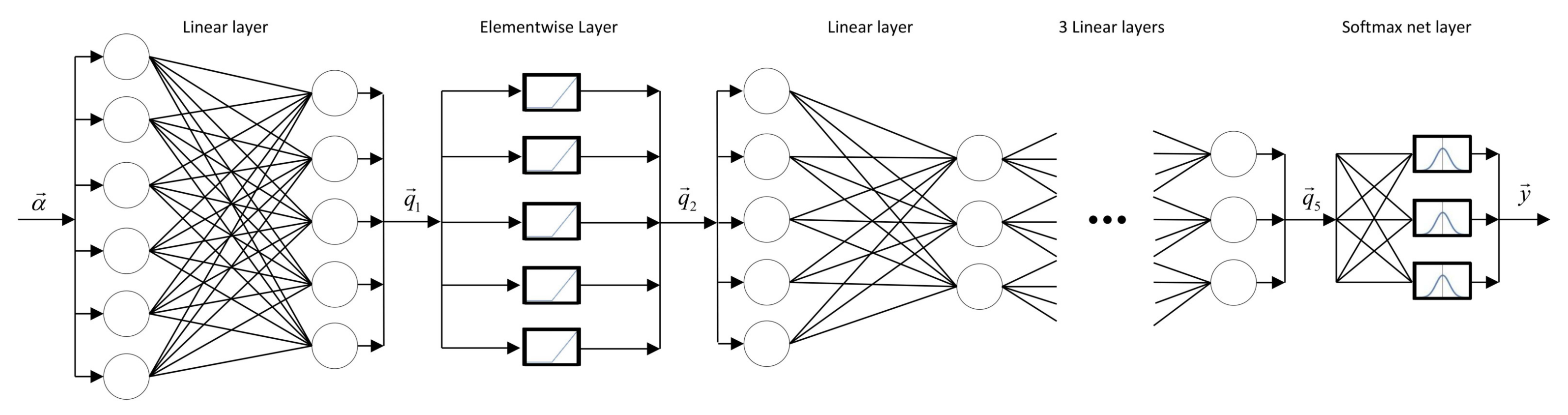The network is decomposed into 6 layers as illustrated in Figure 4, each of which represents a different function mapping vectors to vectors. The successive layers are: a linear layer with an output vector of size k, a nonlinear elementwise activation layer, other three linear layers with output vectors of size k and a nonlinear normalisation layer.

Figure 4. Architecture of the neural network.

The first layer is an affine transformation

$${\overrightarrow{q}}_1=W_1\overrightarrow{\alpha }+{\overrightarrow{b}}_1,$$

where ${\overrightarrow{q}}_1={\mathbb{R}}^{2m+1}$ is the output vector, $W\in {\mathbb{R}}^{2m+1\times k=30}$ is the weight matrix, ${\overrightarrow{b}}_1\in {\mathbb{R}}^{2m+1}$ is the bias vector. The rows in $W_1$ are interpreted as features that are relevant for differentiating between corresponding classes. Consequently, $W_1\overrightarrow{\alpha }$ is a projection of the input $\overrightarrow{\alpha }$ onto these features. The second layer is an elementwise activation layer which is defined by the nonlinear function ${\overrightarrow{q}}_2=max(0,{\overrightarrow{q}}_1)$ setting negative entries of $q_1$ to zero and uses only positive entries. The next three layers are other affine transformations,

$${\overrightarrow{q}}_i=W_i{\overrightarrow{q}}_{i-1}+\overrightarrow{b_i},$$

where ${\overrightarrow{q}}_i\in {\mathbb{R}}^k$, $W_i\in {\mathbb{R}}^{k\times k}$, and $b_i\in {\mathbb{R}}^k$, $i=3,4,5$. The last layer is the normalisation layer $\overrightarrow{y}=softmax\left({\overrightarrow{q}}_5\right)$, whose componentwise is of the form

$$y_N=\frac{e^{q_{5N}}}{{\sum }_N{e}^{q_{5N}}},N=1,\cdots ,N_c.$$

The last layer normalises the output vector $\overrightarrow{y}$ with the aim to get the values between 0 and 1. The output $\overrightarrow{y}$ can be treated as a probability distribution vector, where the Nth element $y_N$ represents the likelihood that $\overrightarrow{\alpha }$ belongs to class N.

We use 70% of the same data S which was not used to verify the quality of the HS in a training phase of the NN and the rest of S—as validation data. We train a multilayer (6-layer) NN using an adaptive moment estimation method [24] and the neural network toolbox in Mathematica© of the Wolfram Research. Then we verify the approximated function

$${\widehat{q}}_k:={\widehat{q}}_k(\lambda ,{\mu }_1,\cdots ,{\mu }_K,c_0,c_1,\cdots ,c_K),$$

which should be accurate enough to be used to predict new output from verification data. The algorithm was ran many times on samples and networks with different sizes. In all cases the results were quite positive and indicate the potential of machine learning methodology for optimisation problems in the queueing theory.

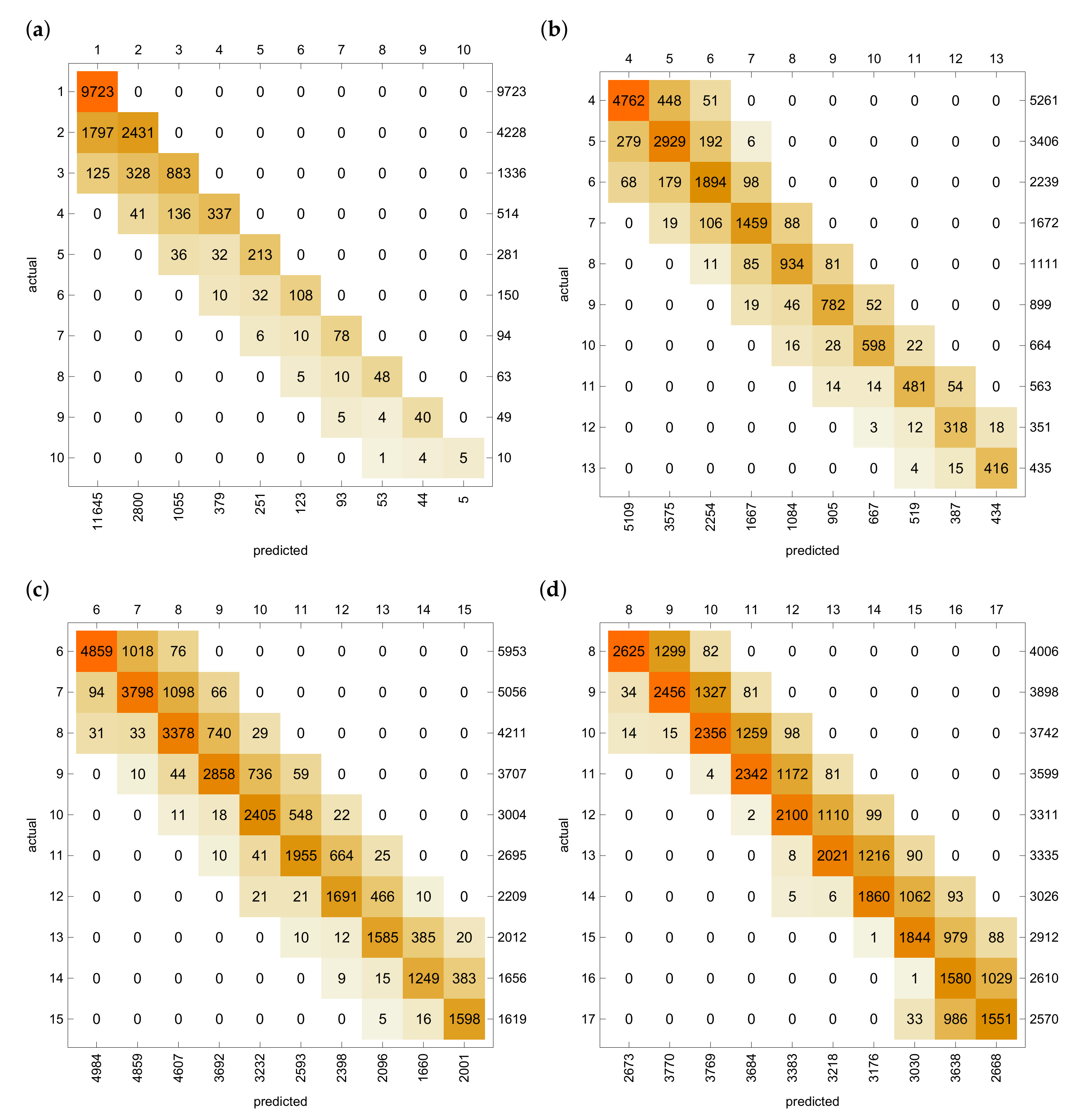
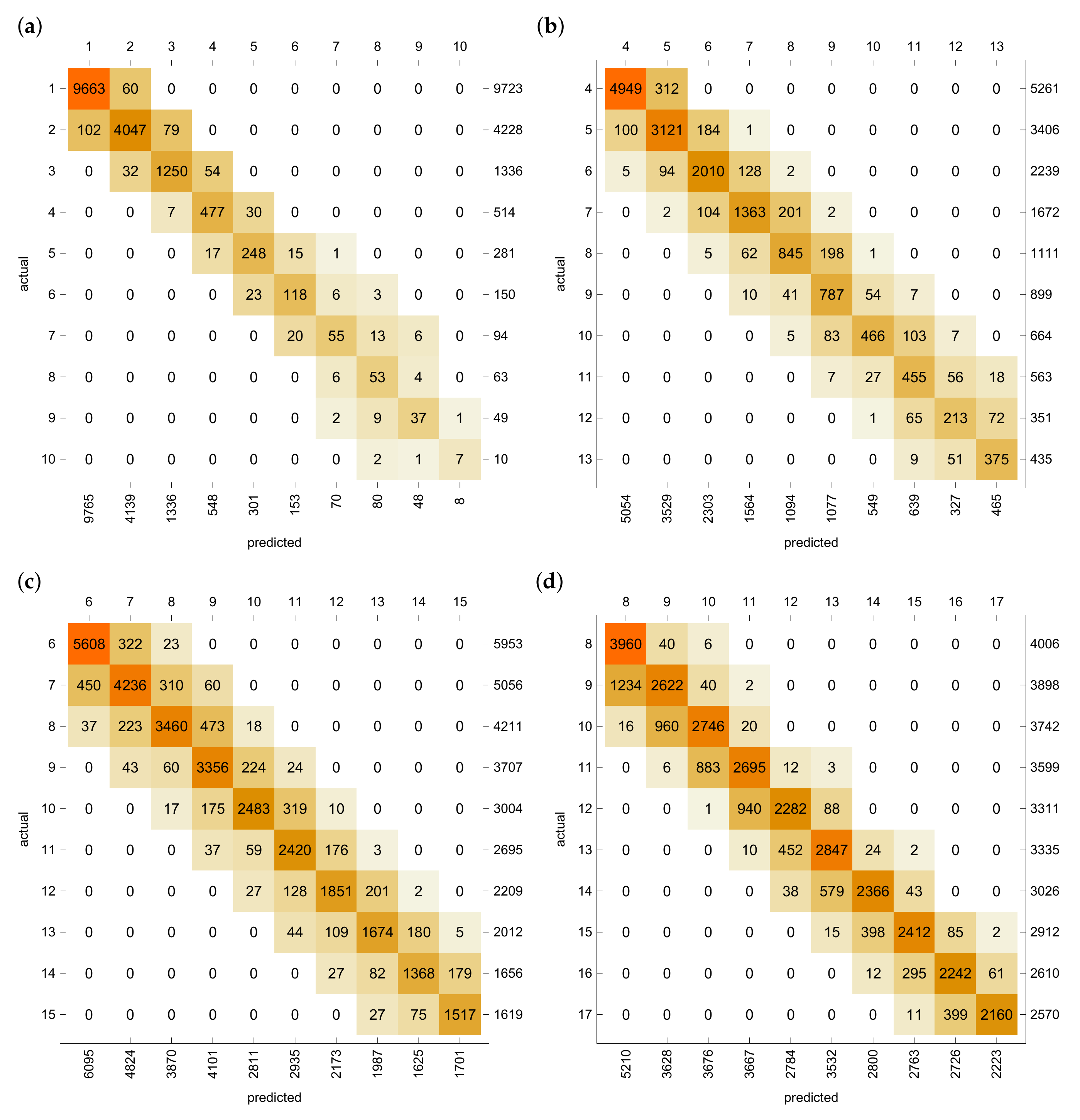
Example 5.

The results of estimations of the optimal threshold values using the trained NN are summarised again in form of confusion matrices, as is shown in Figure 5. The overall accuracy of classification and accuracies for the values with deviations are given in Table 5. We can see that the NN methodology exhibits even more accurate estimations for the optimal thresholds if the results are compared with the corresponding HS.

Figure 5. Confusion matrices (a–d) for prediction of $q_2,q_3,q_4$ and $q_5$ using NN.

Table 5. Accuracy for prediction with NN.

NN	${\mathit{q}}_2$	${\mathit{q}}_3$	${\mathit{q}}_4$	${\mathit{q}}_5$
Accuracy	0.9700	0.8785	0.8708	0.7977
Accuracy $\pm 1$	0.9991	0.9951	0.9874	0.9962

5. Conclusions

We combine classic methodology of analysing controllable queues with a heuristic solution and machine learning to study the possibility to estimate the values of optimal thresholds. Due to the fact that the results were quite positive, we can make the following general conclusion. With this study we confirm that the analysis of controlled queueing systems and the solution of optimisation problems using classical Markov decision theory can be successfully combined with machine learning techniques. These approaches do not contradict each other; on the contrary, combining them provides new results.