On a Generalization of One-Dimensional Kinetics

Abstract

One-dimensional random walks with a constant velocity between scattering are considered. The exact solution is expressed in terms of multiple convolutions of path-distributions assumed to be different for positive and negative directions of the walk axis. Several special cases are considered when the convolutions are expressed in explicit form. As a particular case, the solution of A. S. Monin for a symmetric random walk with exponential path distribution and its generalization to the asymmetric case are obtained. Solution of fractional telegraph equation with the fractional material derivative is presented. Asymptotic behavior of its solution for an asymmetric case is provided.

1. Introduction

The main difference between the Boltzmann kinetic equation and widely used diffusion approximation is the velocity loss. Whereas the Boltzmann trajectory is a broken line consisting of rectilinear segments, each of which is characterized by a certain velocity, and any part of the trajectory has a length and travel time, a Brownian particle in the Wiener representation has a continuous everywhere but nowhere differentiable trajectory. The length of its section between any two points is infinite. From a physical point of view, some of the consequences of this approximation are unacceptable. Particularly, a small diffusion packet placed in an infinite medium will instantly spread to all space that conflicts with special relativity. This is the price to pay for the ease of a mathematical solution.

To the best of our knowledge, the first who undertook an attempt to involve a finite velocity into this model was Soviet physicist-theorist V. A. Fock [1]. His aim was to describe the diffusion of light in a medium with small transparent reflecting particles suspended in it. Beginning his article with consideration of the random hopping process on a discrete system of nodes, he formulated the mathematical problem by means of algebraic equations and gave its solution in terms of finite differences, and only to the end of his article, Fock introduced a finite constant velocity c (he considered photons) and derived the system of differential interrelations under the Markovian assumption that the probability for the particle changing its motion direction into the opposite one during interval $(t,t+dt)$ is equal to $\mu dt$:

$$p_{+}(x,t)=p_{+}(x-cdt,t-dt)(1-\mu dt)+p_{-}(x+cdt,t-dt)\mu dt,$$

(1)

$$p_{-}(x,t)=p_{-}(x+cdt,t-dt)(1-\mu dt)+p_{+}(x-cdt,t-dt)\mu dt.$$

(2)

This pair of equalities is a one-dimensional case of the linear Boltzmann equation expressed through differentials. Each of these two functions obeys an equation of the wave-type

$$\frac{{\partial }^{2}u}{\partial x^2}=\frac{1}{c^2}\frac{{\partial }^{2}u}{\partial t^2}+\frac{1}{D}\frac{\partial u}{\partial t},$$

(3)

called the telegraph equation. The presence of term $\frac{1}{c^2}\frac{{\partial }^{2}u}{\partial t^2}$ shows that any perturbations and inhomogeneities in concentration spreads with the finite velocity c, but after they become smooth, the next development of the process is governed by the ordinary diffusion equation. Ten years later, another Soviet physicist published his article on the same problem [2]. Beginning with the remark that the ordinary diffusion equation is derived under the assumption of the infinite velocity of free motion between collisions, Fock took into account the duration of a free path. However, at the molecular level, the proposed interpretation looks convincing only on the condition that the medium in question is a fairly rarefied gas of short-interacting molecules. It is also not applicable to real particles observed by Brown and later by Perrin (1909) under a microscope, because the suspended particles are much larger in size than molecules and are under their continuous collective action, which does not disintegrate into separate collisions. Only nowadays there exist a technique that made it possible to measure the instantaneous velocities of molecules between collisions [3]. Understanding this situation made physicists shift their attention from molecular diffusion to the turbulent one, in which it is easy to observe the velocities of test particles (tracers) carried by the turbulent flow and to measure them.

In [4], A.S. Monin significantly advanced the understanding of the possibilities of the model under consideration by applying it to the description of turbulent diffusion, relying on the fundamental work of A. N. Kolmogorov [5]. Within the framework of the Kolmogorov picture, the turbulent diffusion of a tracer can be regarded as the result of thin action flows, i.e., jets, randomly distributed in fluid. In the presence of only two types of jets with opposite directions of their motion and on the assumption that random transitions of the tracer from one jet to another form the Poisson process, this random motion is described by the telegraph equation. Taking for initial direction of velocity probabilities $P(+)={\epsilon }_1,$$P(-)={\epsilon }_2$, Monin obtained the spatial distribution of the walking particle along the x-axis in the form

$$p(x,t)=p^{\left(0\right)}(x,t)+p^{\left(s\right)}(x,t),$$

where

$$p^{\left(0\right)}(x,t)=e^{-\mu t}\left[{\epsilon }_1\delta (x-vt)+{\epsilon }_2\delta (x+vt)\right]$$

is the unscattered part, and $p^{\left(s\right)}(x,t)$ is the scattered one, expressed through the modified Bessel functions with argument $\mu t\sqrt{1-{(x/vt)}^2}$, where $-vt<x<vt$.

A fundamentally important circumstance accompanying the derivation of the telegraph equation is the proportionality of the scattering probability on an elementary path to the length of this path, the result of which is the exponential type of the free path distribution. In a review [6], a detailed analysis of Einstein’s derivation of diffusion equation was done and revealed an important circumstance taking place in the case with the telegraph equation as well: random positions of scatterers acting on the tracer are considered to be statistically independent. In other words, these equations model passing a tracer through an ideal gas, molecules of which do not interact with each other, so there are no correlations between consecutive collisions. Certainly, the inertia of the tracer possessing some mass produces some small correlations, especially in a rarified matter, but much stronger correlations arise in a turbulent media, when the tracer is picked up by the random flow (having the form of a jet or vortex) and carried to large distances. A similar situation takes place in the case of charged particle diffusion in random magnetic fields, correlations of which are produced by a random system of magnetic force lines. Some of these cases allow the broken-line approximation of certain parts of the trajectory, but the lengths of the random segments have distributions that differ from the classical exponential form.

We consider in this paper other examples of one-dimensional random motion also admitting a rather easy solution but being beyond the Markovian paradigm. In a general case, we should be ready to describe a process by means of using integral operators with an arbitrary kernel and find a way to its solution. Such an approach is known as the nonlocal transport theory and find a more and more broadening field of applications.

2. The Generalized Process

One-dimensional walking of a particle under consideration starts from the point $x=0$ at the moment $t=0$ with probability ${\epsilon }_1$ on the left (towards negative x) and with probability ${\epsilon }_2=1-{\epsilon }_1$ in the opposite direction. Velocities of free motion in different directions are also different and are of $v_1$ and $v_2$ correspondingly. The probability density for a random free path (to the point of changing the direction of the motion) depends on direction as well and is denoted by $p_1^{\prime }\left(\xi \right)$ for the left direction and $p_2^{\prime }\left(\xi \right)$ for the right ($\xi >0$). The problem is to determine the probability density $\rho (x,t)$ of the particle coordinate at the moment $t>0$.

A further modification of this scheme is possible by introduction of a square matrix ${\epsilon }_{ij}$, determining the transition probability from the state of motion j to the state i ($i,j=1,2$). Let us denote the path-distribution in this modifications $q_i\left(\xi \right)$, so free path distributions become

$$p_i^{\prime }\left(\xi \right)={\epsilon }_{ij}\sum _{n=1}^{\infty }{\epsilon }_{ii}^{n-1}{q}_i^{\left(n\right)}\left(\xi \right),i\ne j$$

(4)

where $q_i^{\left(n\right)}\left(\xi \right)$ denotes multiple convolutions of the densities $q_i\left(\xi \right)$:

$$q_i^{\left(1\right)}\left(\xi \right)=q_i\left(\xi \right),q_i^{(n+1)}\left(\xi \right)=\underset{0}{\overset{\xi }{\int }}{q}_i^{\left(n\right)}(\xi -{\xi }^{\prime })q_i\left({\xi }^{\prime }\right)d{\xi }^{\prime }.$$

(5)

The sought density consists of two parts

$$\rho (x,t)={\rho }_1(x,t)+{\rho }_2(x,t)$$

(6)

corresponding to possible directions (states) of particle motion. Denote by $\xi$ the distance between points of observation and the appearance of the particle in some state via transition from another state or emitted by a source. The minimum value of $\xi$ is zero, and the maximum value depends on $x,t$ and a considered state. For state 1, it satisfies the system of equations

$$\begin{array}{c}\hfill x+\xi =v{t}^{*}\\ \hfill \xi =v(t-t^{*})\end{array}$$

(7)

where $t^{*}$ is the moment of time when the particle performs a jump from a corresponding point of the cone ($x=-vt,x=vt$) to the point x. Excluding $t^{*}$, we find

$${\left({\xi }_{max}\right)}_1=(vt-x)/2\equiv {\xi }_1(x,t).$$

(8)

Similarly, for state 2, we find

$${\left({\xi }_{max}\right)}_2=(vt+x)/2\equiv {\xi }_2(x,t).$$

(9)

Let $f_1(x^{\prime },t^{\prime })d{x}^{\prime }d{t}^{\prime }$ be the probability of particle appearance in state 1 in the element $d{x}^{\prime }$ during $d{t}^{\prime }$ and let $P_1(x^{\prime },t^{\prime }\to x,t)$ be the probability that it will pass a segment $[x,x^{\prime }]$ without collisions and at time t turns out to be at point x:

$$P_1(x^{\prime },t^{\prime }\to x,t)=P_1\left(\xi \right)\delta (t-t^{\prime }-\xi /v),\xi =x^{\prime }-x.$$

(10)

Here

$$P_1\left(\xi \right)=\underset{\xi }{\overset{\infty }{\int }}{p}_1\left(x\right)dx$$

(11)

stands for probability that the random path of the particle will exceed $\xi \ge 0$. The first density component is expressed through the integral

$${\rho }_1(x,t)=(1/v)\underset{x}{\overset{vt}{\int }}d{x}^{\prime }\underset{0}{\overset{t}{\int }}d{t}^{\prime }{f}_1(x^{\prime },t^{\prime })P_1(x^{\prime },t^{\prime }\to x,t)$$

(12)

having the sense of the absolute value of the current particle $j_1$ in the direction 1, so $j_1=v{\rho }_1$. Inserting (10) into (12) and using the $\delta$-function property, we arrive at expression

$${\rho }_1(x,t)=(1/v)\underset{0}{\overset{{\xi }_1(x,t)}{\int }}d\xi P_1\left(\xi \right)f_1(x+\xi ,t-\xi /v).$$

(13)

Considering in a similar way the motion in the opposite direction, we find the second relation:

$${\rho }_2(x,t)=(1/v)\underset{0}{\overset{{\xi }_2(x,t)}{\int }}d\xi P_2\left(\xi \right)f_2(x-\xi ,t-\xi /v).$$

(14)

The collision densities $f_i(x,t)$ satisfy the system of integral equations, derived from the same reasoning as (13) and (14), and have the form

$$f_1(x,t)=\underset{0}{\overset{{\xi }_2(x,t)}{\int }}d\xi p_2\left(\xi \right)f_2(x-\xi ,t-\xi /v)+f_1^{\left(0\right)}(x,t)$$

(15)

$$f_2(x,t)=\underset{0}{\overset{{\xi }_1(x,t)}{\int }}d\xi p_1\left(\xi \right)f_1(x+\xi ,t-\xi /v)+f_2^{\left(0\right)}(x,t)$$

(16)

The free terms

$$f_i^{\left(0\right)}(x,t)={\epsilon }_i\delta \left(x\right)\delta \left(t\right)$$

(17)

describe the emission of particles by the source.

3. Solving the Generalized Equation

Let us add to ${\rho }_{ij}$ and $f_{ij}$ the second index, indicating a fixed initial state of the particle, so

$${\rho }_i(x,t)={\rho }_{i1}(x,t){\epsilon }_1+{\rho }_{i2}(x,t){\epsilon }_2$$

(18)

After one iteration, the system of equations for $f_{ij}(x,t)$ (15)–(16) become a pair of independent equations

$$f_{1j}(x,t)=f_{1j}^{\left(0\right)}(x,t)+\underset{0}{\overset{{\xi }_2(x,t)}{\int }}d\xi p_2\left(\xi \right)\underset{0}{\overset{{\xi }_1(x,t)}{\int }}d{\xi }^{\prime }{p}_1\left({\xi }^{\prime }\right)f_{1j}(x-\xi +{\xi }^{\prime },t-(\xi +{\xi }^{\prime })/v)$$

(19)

$$f_{2j}(x,t)=f_{2j}^{\left(0\right)}(x,t)+\underset{0}{\overset{{\xi }_1(x,t)}{\int }}d\xi p_1\left(\xi \right)\underset{0}{\overset{{\xi }_2(x,t)}{\int }}d{\xi }^{\prime }{p}_2\left({\xi }^{\prime }\right)f_{2j}(x+\xi -{\xi }^{\prime },t-(\xi +{\xi }^{\prime })/v)$$

(20)

with free terms

$$\begin{array}{c}\hfill f_{11}(x,t)=f_{22}(x,t)=\delta \left(x\right)\delta \left(t\right),\\ \hfill f_{21}(x,t)=p_1\left(vt\right)\delta (t+x/v),\\ \hfill f_{12}(x,t)=p_2\left(vt\right)\delta (t-x/v).\end{array}$$

(21)

Let us consider the equation for $f_{11}(x,t)$ in detail, omitting lower indexes to be short. Representing its solution in the form of von Neumann series, we obtain

$$f(x,t)=\sum _{n=0}^{\infty }{f}^{\left(n\right)}(x,t),$$

(22)

where

$$f^{(n+1)}(x,t)=\underset{0}{\overset{{\xi }_2(x,t)}{\int }}d\xi p_2\left(\xi \right)\underset{0}{\overset{{\xi }_1(x,t)}{\int }}d{\xi }^{\prime }{p}_1\left({\xi }^{\prime }\right)f^{\left(n\right)}(x+{\xi }^{\prime }-\xi ,t-({\xi }^{\prime }+\xi )/v).$$

(23)

For the farther exposition, it is convenient to extend the notion of multiple convolution

$$p_i^{(n+1)}\left(\xi \right)=\underset{0}{\overset{\xi }{\int }}{p}_i^{\left(n\right)}(\xi -{\xi }^{\prime })p_i\left({\xi }^{\prime }\right)d{\xi }^{\prime }$$

(24)

to the case $n=0$:

$$p_i^{\left(0\right)}\left(\xi \right)=\delta \left(\xi \right).$$

(25)

A simple check confirms that

$$f^{\left(0\right)}(x,t)=(v/2)p_1^{\left(0\right)}\left({\xi }_1\right)p_2^{\left(0\right)}\left({\xi }_2\right).$$

(26)

Substituting (26) into (23) and finding a few first iterations, we see that each term has the form of a product

$$f^{\left(n\right)}(x,t)={\psi }_n^{(-)}\left({\xi }_1\right){\psi }_n^{(+)}\left({\xi }_2\right).$$

(27)

Substituting (27) into (23) and taking into account that

$${\xi }_2(x+{\xi }^{\prime }-\xi ,t-({\xi }^{\prime }+\xi )/v)={\xi }_2(x,t)-\xi$$

(28)

and

$${\xi }_1(x+{\xi }^{\prime }-\xi ,t-({\xi }^{\prime }+\xi )/v)={\xi }_1(x,t)-\xi$$

(29)

yields

$${\psi }_{n+1}^{(+)}\left({\xi }_2\right)=\underset{0}{\overset{{\xi }_2}{\int }}d\xi p_2\left(\xi \right){\psi }_n^{(+)}({\xi }_2-\xi )$$

(30)

and

$${\psi }_{n+1}^{(-)}\left({\xi }_1\right)=\underset{0}{\overset{{\xi }_1}{\int }}d\xi p_1\left(\xi \right){\psi }_n^{(-)}({\xi }_1-\xi ).$$

(31)

4. Solution of the Generalized Equation for the Process with an Arbitrary Transition Density

The latter functions are expressed in terms of multiple convolutions of distributions $p_1\left(\xi \right)$ and $p_2\left(\xi \right)$, so we have:

$$f(x,t)=f_{11}(x,t)=(v/2)\sum _{n=0}^{\infty }{p}_1^{\left(n\right)}\left({\xi }_1\right)p_2^{\left(n\right)}\left({\xi }_2\right).$$

(32)

The meaning of the summation index n is clear: it is the number of particle steps after which it appears in state 1 at point x at moment t. Since the initial state is also 1, the probability that after some (any) number of steps n the particle will be at state 1 without reference to x and t, is equal to 1. It is easy to verify that this normalization condition is satisfied. Expressing ${\xi }_1$ through ${\xi }_2$ using relation ${\xi }_1=vt-{\xi }_2$ yields

$$\begin{array}{c}\hfill (v/2)\underset{0}{\overset{\infty }{\int }}dt\underset{-vt}{\overset{vt}{\int }}dx{p}_1^{\left(n\right)}(vt-{\xi }_2)p_2^{\left(n\right)}\left({\xi }_2\right)=v\underset{0}{\overset{\infty }{\int }}dt\underset{0}{\overset{vt}{\int }}d{\xi }_2{p}_1^{\left(n\right)}(vt-{\xi }_2)p_2^{\left(n\right)}\left({\xi }_2\right)\\ \hfill =\underset{0}{\overset{\infty }{\int }}d{\xi }_2{p}_2^{\left(n\right)}\left({\xi }_2\right)\underset{0}{\overset{\infty }{\int }}d{\xi }_1{p}_1^{\left(n\right)}\left({\xi }_1\right)=1.\end{array}$$

(33)

Similarly, we get function $f_{21}(x,t)$, but since the right side of the corresponding equation has the form

$$f_{21}^{\left(0\right)}(x,t)=(v/2)p_1^{\left(1\right)}\left({\xi }_1\right)p_2^{\left(0\right)}\left({\xi }_2\right)$$

(34)

the result will be

$$f_{21}(x,t)=(v/2)\sum _{n=0}^{\infty }{p}_1^{(n+1)}\left({\xi }_1\right)p_2^{\left(n\right)}\left({\xi }_2\right).$$

(35)

We also give the expressions for the other two functions:

$$f_{12}(x,t)=(v/2)\sum _{n=0}^{\infty }{p}_1^{\left(n\right)}\left({\xi }_1\right)p_2^{(n+1)}\left({\xi }_2\right)$$

(36)

and

$$f_{22}(x,t)=(v/2)\sum _{n=0}^{\infty }{p}_1^{\left(n\right)}\left({\xi }_1\right)p_2^{\left(n\right)}\left({\xi }_2\right).$$

(37)

However, it is clear from obvious reasons that $f_{12}$ can be obtained from $f_{21}$, and $f_{22}$ from $f_{11}$, by replacing all lower indexes $(1\to 2,2\to 1)$ in the right side of expressions (35) and (32), respectively. Substituting the expressions found in the right sides of (13), (14) and considering that

$$\begin{array}{c}\hfill \underset{0}{\overset{{\xi }_1}{\int }}d\xi P_1\left(\xi \right)p_1^{\left(n\right)}({\xi }_1-\xi )=\underset{0}{\overset{{\xi }_1}{\int }}d\xi p_1^{\left(n\right)}({\xi }_1-\xi )-\underset{0}{\overset{{\xi }_1}{\int }}d\xi F_1\left(\xi \right)p_1^{\left(n\right)}({\xi }_1-\xi )\\ \hfill =F_1^{\left(n\right)}\left({\xi }_1\right)-F_1^{(n+1)}\left({\xi }_1\right)\equiv \Delta F_1^{\left(n\right)}\left({\xi }_1\right)\end{array}$$

(38)

and

$$\underset{0}{\overset{{\xi }_2}{\int }}d\xi P_2\left(\xi \right)p_2^{\left(n\right)}({\xi }_2-\xi )=\Delta F_2^{\left(n\right)}\left({\xi }_2\right)$$

(39)

where

$$F_i^{\left(n\right)}\left(\xi \right)=\underset{0}{\overset{\xi }{\int }}{p}_i^{\left(n\right)}\left(x\right)dx$$

(40)

is a distribution function, we shall get

$${\rho }_{11}(x,t)=(1/2)\sum _{n=0}^{\infty }\Delta F_1^{\left(n\right)}\left({\xi }_1\right)p_2^{\left(n\right)}\left({\xi }_2\right)$$

(41)

$${\rho }_{21}(x,t)=(1/2)\sum _{n=0}^{\infty }{p}_1^{(n+1)}\left({\xi }_1\right)\Delta F_2^{\left(n\right)}\left({\xi }_2\right).$$

(42)

As in the case of $f_{ij}(x,t)$, expressions for densities ${\rho }_{22}(x,t)$ and ${\rho }_{12}(x,t)$ are obtained from (41)–(42) by permutation of the lower indexes. Note that the distribution presented here includes $\delta$-features, given by the term with $n=0$, so the normalization condition is valid:

$$\underset{-vt}{\overset{vt}{\int }}\left[{\rho }_{1i}(x,t)+{\rho }_{2i}(x,t)\right]dx=1.$$

(43)

The representation (41)–(42) of the walking problem reduces it to a calculation of multiple convolutions $p_1^{\left(n\right)}\left(x\right)$ and $p_2^{\left(n\right)}\left(x\right)$ of path-densities. We divide the set of such distributions into four classes: A, whose convolutions are expressed in terms of elementary or special functions; B, whose convolutions are expressed in terms of the original one with changed parameters; and C, whose convolutions are expressed through the initial one up to the linear scale transform (Lévy-stable densities). Below, we consider some of them. Taking any of these distributions allows us to get the solution in a closed form. Finally, the last (D) class includes densities, producing solutions with self-similar (with respect to space-time variables) long-time asymptotics.

5. Solution for the Process with Exponential and Gamma-Distributions

We begin the search for explicit solutions with the simplest term of this family

$$p_i\left(\xi \right)={\mu }_i{e}^{-{\mu }_i\xi },{\mu }_1\ne {\mu }_2$$

(44)

In this case

$$p_i^{\left(n\right)}\left(\xi \right)={\mu }_i\frac{{\left({\mu }_i\xi \right)}^{n-1}}{(n-1)!}{e}^{-{\mu }_i\xi }$$

(45)

and

$$\Delta F_i^{\left(n\right)}\left(\xi \right)\equiv F_i^{\left(n\right)}\left(\xi \right)-F_i^{(n+1)}\left(\xi \right)=\frac{{\left({\mu }_i\xi \right)}^n}{n!}{e}^{-{\mu }_i\xi }$$

(46)

Substituting these expressions into (41), we obtain for the regular component ($n\ne 0$)

$$\begin{gathered} {\tilde{\rho }}_{11}(x,t)=(1/2)\sum _{n=1}^{\infty }\frac{{\left({\mu }_1{\xi }_1\right)}^n}{n!}{\mu }_2\frac{{\left({\mu }_2{\xi }_2\right)}^{n-1}}{(n-1)!}{e}^{-{\mu }_1{\xi }_1-{\mu }_2{\xi }_2} \\ =(1/2){\mu }_1{\mu }_2{\xi }_1{e}^{-{\mu }_1{\xi }_1-{\mu }_2{\xi }_2}\sum _{n=1}^{\infty }\frac{{\left({\mu }_1{\xi }_1{\mu }_2{\xi }_2\right)}^n}{(n+1)!n!} \end{gathered}$$

(47)

The last sum is an expansion to the power series of $(2/z)I_1\left(z\right)$ function, where

$$z=2\sqrt{{\mu }_1{\xi }_1{\mu }_2{\xi }_2}=\sqrt{{\mu }_1{\mu }_2\left[{\left(vt\right)}^2-x^2\right]}$$

(48)

As a result, we have

$${\tilde{\rho }}_{11}(x,t)=\frac{\sqrt{{\mu }_1{\mu }_2}(vt-x)}{2\sqrt{{\left(vt\right)}^2-x^2}}exp\{-({\mu }_1+{\mu }_2)vt/2-({\mu }_2-{\mu }_1)x/2\}{I}_1\left(\sqrt{{\mu }_1{\mu }_2\left[{\left(vt\right)}^2-x^2\right]}\right)$$

(49)

Similary, from (42) we find

$${\tilde{\rho }}_{21}(x,t)=({\mu }_1/2)exp\{-({\mu }_1+{\mu }_2)vt/2-({\mu }_2-{\mu }_1)x/2\}{I}_0\left(\sqrt{{\mu }_1{\mu }_2\left[{\left(vt\right)}^2-x^2\right]}\right)$$

(50)

The components ${\tilde{\rho }}_{22}(x,t)$ and ${\tilde{\rho }}_{12}(x,t)$ are obtained by changing indices of the coefficients $\mu$ and changing the sign before x. The total distribution

$$\tilde{\rho }(x,t)=\left[{\tilde{\rho }}_{11}(x,t)+{\tilde{\rho }}_{21}(x,t)\right]{\epsilon }_1+\left[{\tilde{\rho }}_{12}(x,t)+{\tilde{\rho }}_{22}(x,t)\right]{\epsilon }_2$$

(51)

reads for $x\in (-vt,vt)$:

$$\tilde{\rho }(x,t)=\{\left[({\mu }_1{\epsilon }_1+{\mu }_2{\epsilon }_2)/2\right]I_0\left(\sqrt{{\mu }_1{\mu }_2\left[{\left(vt\right)}^2-x^2\right]}\right).+\left.\frac{\sqrt{{\mu }_1{\mu }_2}\left[vt+({\epsilon }_2-{\epsilon }_1)x\right]}{2\sqrt{{\left(vt\right)}^2-x^2}}{I}_1\left(\sqrt{{\mu }_1{\mu }_2\left[{\left(vt\right)}^2-x^2\right]}\right)\right\}\times$$

$$\times exp\{-({\mu }_1+{\mu }_2)vt/2-({\mu }_2-{\mu }_1)x/2\}.$$

(52)

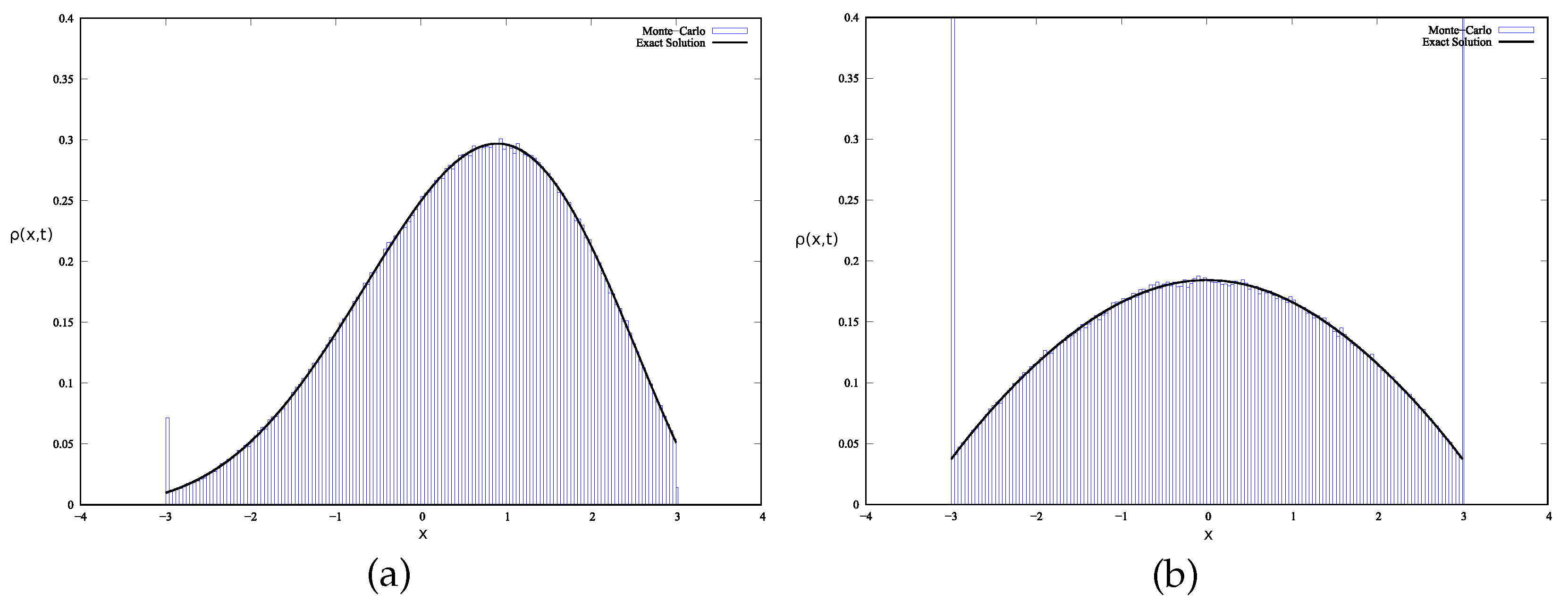
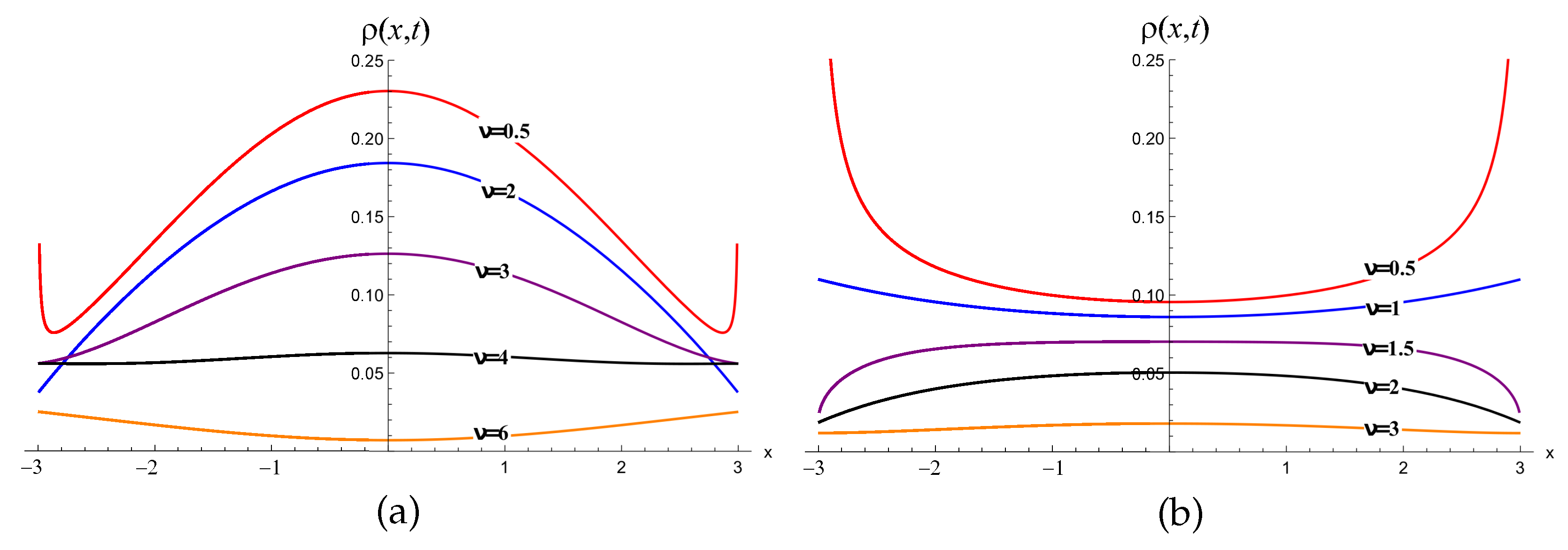
Solutions for exponential and gamma distribution of path lengths are demonstrated in Figure 1. All results were confirmed using Monte Carlo simulations; for example, the result of the modeling for exponential and gamma walks are shown in Figure 2.

Equation (37) is a particular case of the gamma distribution.

$$p_{i,{\nu }_i}\left(\xi \right)={\mu }_i\frac{{\left({\mu }_i\xi \right)}^{{\nu }_i-1}}{\Gamma \left({\nu }_i\right)}{e}^{-{\mu }_i\xi }$$

(53)

The family of gamma distributions is closed under convolution [7]. Therefore, choosing

$$p_i\left(\xi \right)=p_{i,{\nu }_i}\left(\xi \right)$$

(54)

we immediately get

$$p_i^{\left(n\right)}\left(\xi \right)={\mu }_i\frac{{\left({\mu }_i\xi \right)}^{n{\nu }_i-1}}{\Gamma \left(n{\nu }_i\right)}{e}^{-{\mu }_i\xi }$$

(55)

Using (46), we get

$$\Delta F_i^{\left(n\right)}\left(\xi \right)=\frac{\Gamma ([n+1]{\nu }_i,{\mu }_i\xi )}{\Gamma \left([n+1]{\nu }_i\right)}-\frac{\Gamma (n{\nu }_i,{\mu }_i\xi )}{\Gamma \left(n{\nu }_i\right)}$$

(56)

where $\Gamma (\beta ,x)$ is the upper incomplete gamma function. Thus, for regular components of densities ${\rho }_{11}$ and ${\rho }_{21}$, we get

$${\tilde{\rho }}_{11}=\frac{{\mu }_2{e}^{-{\mu }_2{\xi }_2}}{2}\sum _{n=1}^{+\infty }\frac{{\left({\mu }_2{\xi }_2\right)}^{n{\nu }_2-1}}{\Gamma \left(n{\nu }_2\right)}\left(\frac{\Gamma ([n+1]{\nu }_1,{\mu }_1{\xi }_1)}{\Gamma \left([n+1]{\nu }_1\right)}-\frac{\Gamma (n{\nu }_1,{\mu }_1{\xi }_1)}{\Gamma \left(n{\nu }_1\right)}\right)$$

(57)

and

$${\tilde{\rho }}_{21}=\frac{{\mu }_1{e}^{-{\mu }_1{\xi }_1}}{2}\sum _{n=0}^{+\infty }\frac{{\left({\mu }_1{\xi }_1\right)}^{(n+1){\nu }_1-1}}{\Gamma \left([n+1]{\nu }_1\right)}\left(\frac{\Gamma ([n+1]{\nu }_2,{\mu }_2{\xi }_2)}{\Gamma \left([n+1]{\nu }_2\right)}-\frac{\Gamma (n{\nu }_2,{\mu }_2{\xi }_2)}{\Gamma \left(n{\nu }_2\right)}\right)$$

(58)

for integer ${\nu }_i$, this sum can be expressed through integrals of generalized hypergeometric functions. For ${\nu }_1={\nu }_2=2$, these expressions become especially simple

$${\tilde{\rho }}_{11}(x,t)=({\mu }_2/4)\sqrt{{\mu }_1{\xi }_1{\mu }_2{\xi }_2}\left[I_1\left(2\sqrt{{\mu }_1{\xi }_1{\mu }_2{\xi }_2}\right)-J_1\left(2\sqrt{{\mu }_1{\xi }_1{\mu }_2{\xi }_2}\right)\right]exp(-{\mu }_1{\xi }_1-{\mu }_2{\xi }_2)$$

(59)

$${\tilde{\rho }}_{21}(x,t)=({\mu }_1/4)\sqrt{{\mu }_1{\xi }_1/\left({\mu }_2{\xi }_2\right)}\left[I_1\left(2\sqrt{{\mu }_1{\xi }_1{\mu }_2{\xi }_2}\right)+J_1\left(2\sqrt{{\mu }_1{\xi }_1{\mu }_2{\xi }_2}\right)\right]exp(-{\mu }_1{\xi }_1-{\mu }_2{\xi }_2).$$

(60)

6. Solutions for the Process with Some Other Transition Densities

There are some more distributions in which multiple convolutions can be expressed in elementary form, but sums (41) and (42) can not be expressed in closed form (as (57) and (58) with arbitrary ${\nu }_i$). One example is the Bessel density

$$\begin{array}{c}\hfill p_i^{\left(n\right)}\left(\xi \right)={\nu }_i{x}^{-1}{e}^{-\xi }{I}_{{\nu }_i}\left(\xi \right)\\ \hfill p_i^{\left(n\right)}\left(\xi \right)=n{\nu }_i{x}^{-1}{e}^{-\xi }{I}_{n{\nu }_i}\left(\xi \right)\end{array}$$

(61)

Using (46), we get

$$\begin{array}{c}\hfill \begin{array}{c}\hfill \Delta F_i^{\left(n\right)}\left(\xi \right)=2^{-(n+1){\nu }_i}{\xi }^{n{\nu }_i}[2^{{\nu }_i}\Gamma (2n{\nu }_i+1)F_{2;2}(n{\nu }_i,n{\nu }_i+\frac{1}{2};n{\nu }_i+1,2n{\nu }_i+1;-2\xi )-\\ \hfill -\frac{{\xi }^{{\nu }_i}}{\Gamma ({\nu }_i[n+1]+1)}{F}_{2;2}({\nu }_i[n+1],{\nu }_i[n+1]+\frac{1}{2};[n+1]{\nu }_i+1,2[n+1]{\nu }_i+1;-2\xi )]\end{array}\end{array}$$

(62)

where $F_{p;q}(a_1,..,a_p;b_1,..,b_q,x)$ is a generalized hypergeometric function [8]. The sums (41) and (42) can be calculated numerically, and the result are shown in Figure 3.

Another distribution is uniform distribution [7]

$$\begin{array}{c}\hfill p_i\left(\xi \right)=\frac{1}{a_i},0\le \xi \le a_i\\ \hfill p_i^{\left(n\right)}\left(\xi \right)=\frac{1}{(n-1)!a_i^n}\sum _{k=0}^n{(-1)}^k{C}_n^k{(\xi -k{a}_i)}^{n-1}\theta (k{a}_i-\xi ),0\le \xi \le n{a}_i\end{array}$$

(63)

where $\theta \left(x\right)$ is a Heaviside function. For this distribution, we have

$$F_i^{\left(n\right)}\left(\xi \right)=\frac{1}{n!a_i^n}\sum _{k=0}^n{(-1)}^k{C}_n^k[{(\xi -k{a}_i)}^n\theta (k{a}_i-x)-{(-1)}^n{\left(k{a}_i\right)}^n]$$

(64)

and $\Delta F_i^{\left(n\right)}\left(\xi \right)=F_i^{\left(n\right)}\left(\xi \right)-F_i^{(n+1)}\left(\xi \right)$.

A wide class of distributions whose convolutions lie in the same class are one-sided stable densities with $0<\alpha <1$, concentrated on the positive semiaxis [9]

$$\begin{array}{c}\hfill p_i\left(\xi \right)=g^{\left({\alpha }_i\right)}\left(\xi \right)\\ \hfill p_i^{\left(n\right)}\left(\xi \right)=n^{-1/{\alpha }_i}{g}^{\left({\alpha }_i\right)}\left(n^{-1/{\alpha }_i}\xi \right)\end{array}$$

(65)

Using a cumulative distribution function of stable densities $G^{\left(\alpha \right)}\left(x\right)$, we can get

$$\Delta F_i^{\left(n\right)}\left(\xi \right)=G^{\left({\alpha }_i\right)}\left(n^{-1/{\alpha }_i}\xi \right)-G^{\left({\alpha }_i\right)}\left({[n+1]}^{-1/{\alpha }_i}\xi \right)$$

(66)

For a special case $\alpha =1/2$ we have

$$\begin{array}{c}\hfill p^{\left(n\right)}\left(\xi \right)=\frac{n}{2\sqrt{\pi }}{\xi }^{-3/2}{e}^{-\frac{n^2}{4\xi }}\\ \hfill \Delta F^{\left(n\right)}\left(\xi \right)=erf\left(\frac{n+1}{2\sqrt{\xi }}\right)-erf\left(\frac{n}{2\sqrt{\xi }}\right)\end{array}$$

(67)

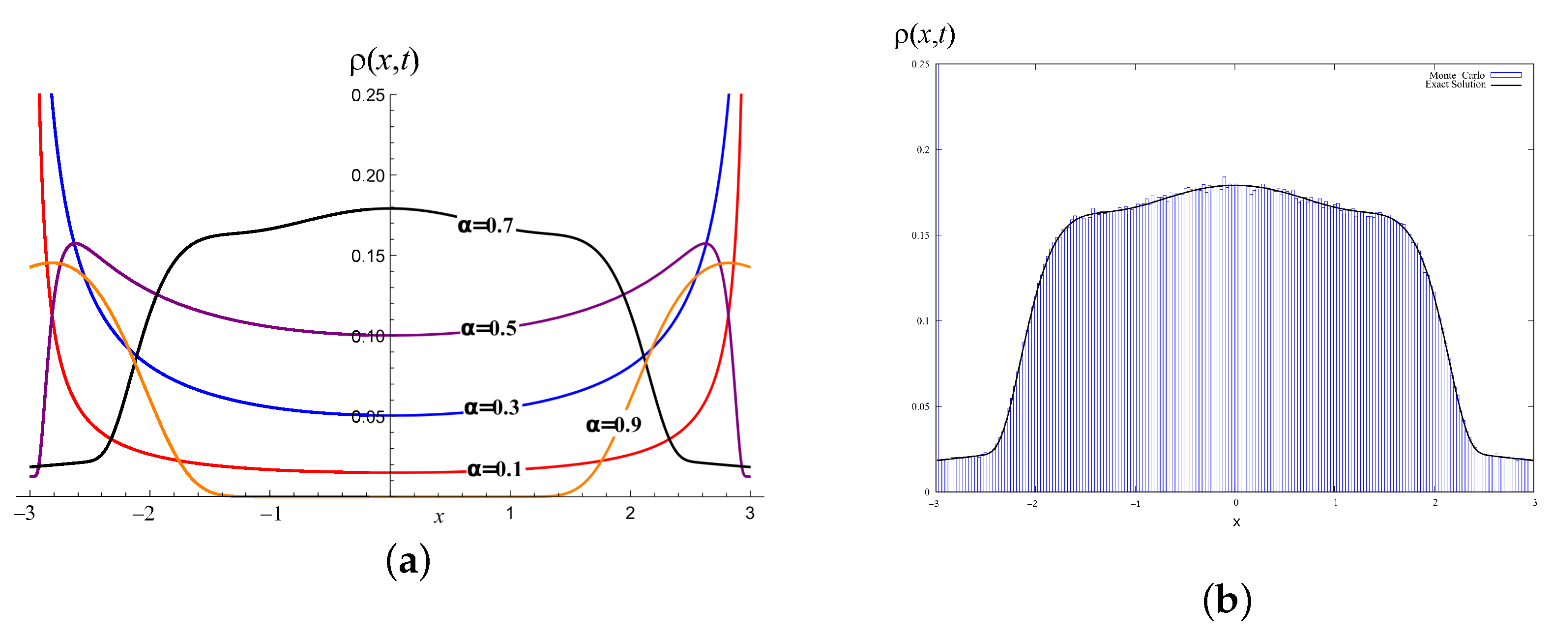
Some distributions with different $\alpha$ are shown in Figure 4a. As in the previous section, all results were proved by means of the Monte Carlo simulations. One example is shown in Figure 4b.

7. Integral Transforms and Asymptotic Results

In the case of an arbitrary density $p\left(z\right)$ with a finite second moment, the asymptotic part of the solution satisfies the telegraph equation. In References [10,11,12], the authors investigated one-dimensional random walks with the asymptotically power-law distribution $p\left(\xi \right)\propto {\xi }^{-\alpha -1}$, $0<\alpha <2$. Such a random process is sometimes called a fractal walk. Recently, Lévy flights with a bi-modal distribution of jumps were studied in Reference [13] and the interesting effect of loss of self-similarity was predicted for certain parameters.

We rewrite Equations (13)–(17) as the following system,

$$\begin{array}{c}\hfill p(x,t)={\int }_0^t[{\gamma }_{1}f(x-v\tau ,t-\tau )+{\gamma }_{2}f(x+v\tau ,t-\tau )]P\left(v\tau \right)d\tau .\end{array}$$

(68)

$$\begin{array}{c}\hfill f(x,t)={\int }_0^t[{\gamma }_{1}f(x-v\tau ,t-\tau )+{\gamma }_{2}f(x+v\tau ,t-\tau )]p\left(v\tau \right)d\tau +\delta \left(x\right)\delta \left(t\right).\end{array}$$

(69)

After the Fourier–Laplace transformation, the solution can be represented as the following transform,

$$\begin{array}{c}\hfill \tilde{p}(k,\lambda )=\frac{\lambda /v-ik\beta -{\gamma }_1(\lambda /v-ik)\tilde{p}(\lambda /v+ik)-{\gamma }_2(\lambda /v+ik)\tilde{p}(\lambda /v-ik)}{v[k^2+{(\lambda /v)}^2][1-{\gamma }_2\tilde{p}(\lambda /v-ik)-{\gamma }_1\tilde{p}(\lambda /v+ik)]}.\end{array}$$

(70)

Consider two cases of fractal walk. Let an asymptotic expansion ($\lambda \to 0$, i.e., $t\to \infty$) of the Laplace transform $\tilde{p}$ be of the form,

$$\begin{array}{c}\hfill \tilde{p}\left(\lambda \right)=1-c{\lambda }^{\alpha },c=(A/\alpha )\Gamma (1-\alpha ),0<\alpha <1.\end{array}$$

(71)

This case corresponds to the heavy-tailed distribution, $p\left(z\right)\sim \alpha {z_0}^{\alpha }{z}^{-\alpha -1},0<\alpha <1$, and all moments of natural order diverge.

Substituting Equation (71) into expression (70), we obtain for the first case

$$\begin{array}{c}\hfill \tilde{p}(k,\lambda )=\frac{{\gamma }_2{(\lambda /v-ik)}^{\alpha -1}+{\gamma }_1{(\lambda /v+ik)}^{\alpha -1}}{v[{\gamma }_2{(\lambda /v-ik)}^{\alpha }+{\gamma }_1{(\lambda /v+ik)}^{\alpha }]},0<\alpha <1.\end{array}$$

(72)

In Reference [12], we inverted this transform in the symmetric case and expressed the result through elementary functions for all values of $\alpha$ of the indicated interval. In the asymmetric case, we have

$$\begin{array}{c}\hfill p(x,t)=\frac{2sin\pi \alpha }{\pi vt}\frac{{\gamma }_1{\gamma }_2{\left(1-x^2/v^2{t}^2\right)}^{\alpha -1}}{{\gamma }_1^2{(1-x/vt)}^{2\alpha }+{\gamma }_2^2{(1+x/vt)}^{2\alpha }+2{\gamma }_1{\gamma }_2{\left(1-x^2/v^2{t}^2\right)}^{\alpha }cos\pi \alpha },0<\alpha <1.\end{array}$$

(73)

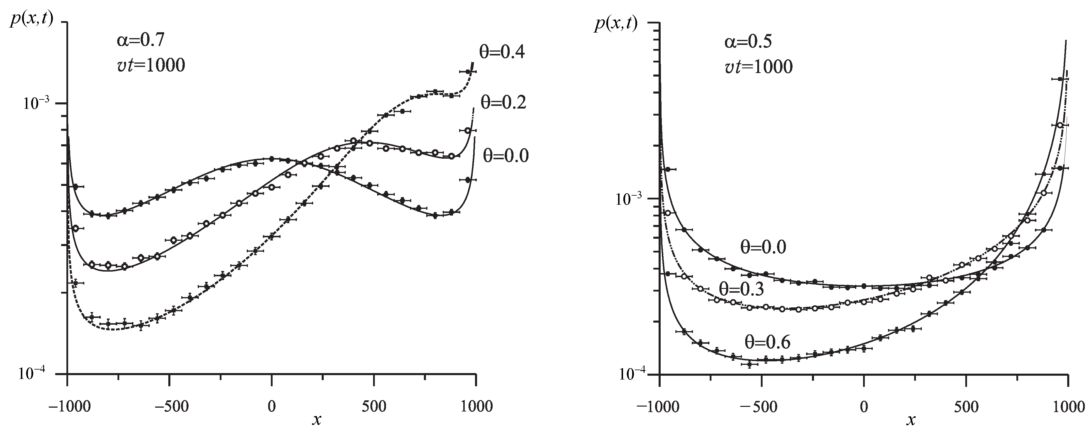
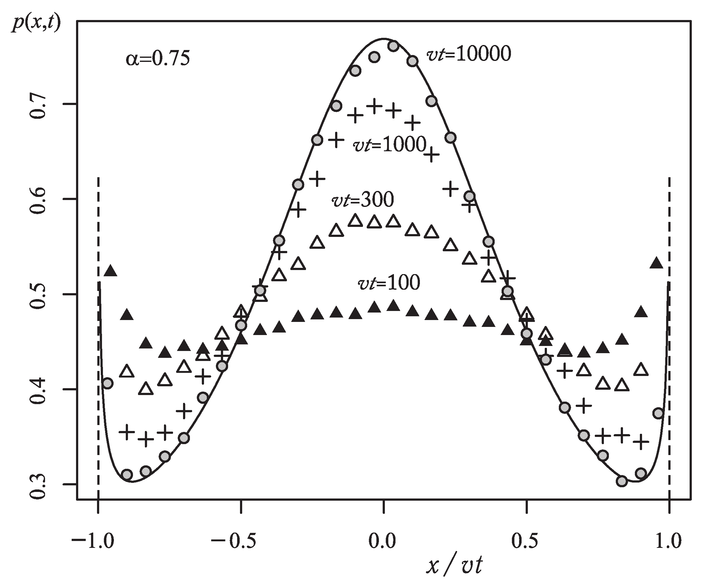
Here, $C={\gamma }_1/{\gamma }_2$. Plots of these distributions for several values of $\alpha$ are presented in Figure 5. The pdf of such type was obtained by Lamperti in frames of the mathematical theory of occupation times [14] and used in statistical physics of weakly non-ergodic systems [15]. Evolution of pdf for instantaneous point source and its tendency to the asymptotic Lamperti distribution ($\alpha =0.75$) is demonstrated in Figure 6. Path lengths are distributed according to the Pareto distribution with the same $\alpha$.

Rewriting relation (72) in the form

$$\begin{array}{c}\hfill v[{\gamma }_2{(\lambda /v-ik)}^{\alpha }+{\gamma }_1{(\lambda /v+ik)}^{\alpha }]\tilde{p}(k,\lambda )={\gamma }_2{(\lambda /v-ik)}^{\alpha -1}+{\gamma }_1{(\lambda /v+ik)}^{\alpha -1}\end{array}$$

(74)

and performing the inverse Fourier–Laplace transformation, we arrive at the equation with material derivatives of fractional order

$$\begin{array}{c}\hfill \left[{\gamma }_2{\left(\frac{\partial }{\partial t}+v\frac{\partial }{\partial x}\right)}^{\alpha }+{\gamma }_1{\left(\frac{\partial }{\partial t}-v\frac{\partial }{\partial x}\right)}^{\alpha }\right]G(x,t)=\frac{t^{-\alpha }}{\Gamma (1-\alpha )}[{\gamma }_2\delta (x+vt)+{\gamma }_1\delta (x-vt)].\end{array}$$

(75)

The multiplier ${(\lambda \pm ivk)}^{\alpha }$ in the formulas derived above presents the Fourier–Laplace transform of the fractional material derivative [11]:

$${(\lambda \mp ivk)}^{\alpha }\tilde{f}(k,\lambda )=\underset{0}{\overset{\infty }{\int }}dt\underset{-\infty }{\overset{\infty }{\int }}dx{e}^{-\lambda t+ikx}{\left(\frac{\partial }{\partial t}\pm v\frac{\partial }{\partial x}\right)}^{\alpha }f(x,t),$$

that can be verified by rewriting the operator in the Riemann–Liouville form:

$${\left(\frac{\partial }{\partial t}\pm v\frac{\partial }{\partial x}\right)}^{\alpha }f(x,t)=\frac{1}{\Gamma (1-\alpha )}\left(\frac{\partial }{\partial t}\pm v\frac{\partial }{\partial x}\right)\underset{0}{\overset{t}{\int }}f(x-v(t-\tau ),\tau ){(t-\tau )}^{-\alpha }d\tau ,0<\alpha <1,$$

and applying the Fourier–Laplace transformation.

The second case is characterized by a finite first moment ($1<\alpha <2$),

$$\begin{array}{c}\hfill \tilde{p}\left(\lambda \right)=1-m_1\lambda +c_1{\lambda }^{\alpha },c_1=\frac{(A/\alpha )\Gamma (2-\alpha )}{\alpha -1},1<\alpha <2.\end{array}$$

(76)

For asymptotic solution, we can put $\lambda \to 0,k\to 0,|\lambda /vk|\to 0$. Thus, the transform takes the following form:

$$\begin{array}{c}\hfill \tilde{p}(k,\lambda )=\frac{1}{\lambda +i\beta kv-(cv/m)\left[{\gamma }_1{\left(ik\right)}^{\alpha }+{\gamma }_2{(-ik)}^{\alpha }\right]}.\end{array}$$

(77)

The inverse Laplace transformation leads to the characteristic function

$$\tilde{p}(k,t)=exp\left(i\beta kvt-\frac{cvt}{m}\left[{\gamma }_1{\left(ik\right)}^{\alpha }+{\gamma }_2{(-ik)}^{\alpha }\right]\right),$$

related to the characteristic function of the Lévy stable density $g(x;\alpha ,\beta )$,

$$\tilde{g}(k;\alpha )=exp\left(-{\left|k\right|}^{\alpha }[1-i\beta tan(\pi \alpha /2)sign\left(k\right)]\right),$$

by the following expression

$$\tilde{p}(k,t)=exp\left(i\beta kvt\right)\tilde{g}({\left(Kt\right)}^{1/\alpha }k;\alpha ;\beta ).$$

The passage to the original leads to the solution:

$$\begin{array}{c}\hfill p(x,t)={\left(Kt\right)}^{-1/\alpha }g\left((x-\beta vt){\left(Kt\right)}^{-1/\alpha };\alpha ,\beta \right),\end{array}$$

(78)

where

$$K=\frac{cv}{m}sin\frac{\pi (\alpha -1)}{2}$$

We rewrite expression (77) in the form

$$\lambda \tilde{p}(k,\lambda )=-i\beta kv\tilde{p}(k,\lambda )+\frac{cv}{m}\left[{\gamma }_1{\left(ik\right)}^{\alpha }+{\gamma }_2{(-ik)}^{\alpha }\right]\tilde{p}(k,\lambda )+1.$$

The inverse Fourier–Laplace transformation of the latter expression corresponds to the superdiffusion equation with a fractional operator.

8. One-Sided Fractal Walks with Traps

In some applications, the models of a random walk with localization events can be useful. Particularly, traps characterized by random waiting times play a major role in the kinetics of dispersive transport of charge carriers in disordered semiconductors [16]. Let us call the localized state off-state, and the state of motion is on-state.

Let $p(x,t)$ be the distribution density of total residence time in on-state. For the double Laplace transform of the density $p(x,t)$,

$$\widehat{\tilde{p}}(k,s)={\int }_0^{\infty }d\tau {\int }_0^{\infty }dtp(\tau ,t)e^{-\tau k-st}.$$

(79)

the following expression is derived [17]:

$$\widehat{\tilde{p}}(k,s)=\frac{v^{-1}\widehat{\psi }\left(s\right)\widehat{P}\left(k+\frac{s}{v}\right)+\widehat{\Psi }\left(s\right)}{1-\widehat{p}\left(k+\frac{s}{v}\right)\widehat{\psi }\left(s\right)}.$$

(80)

Here, v denotes some proportional coefficient responsible for time compression in on-state, $v=1$ if time measures in on- and off- states coincide. Under the assumption of power-law distributions of waiting times in off- and on-states,

$$\widehat{\psi }\left(s\right)\sim 1-{\tau }^{\beta }{s}^{\beta },\widehat{\Psi }\left(s\right)=\frac{1-\widehat{\psi }\left(s\right)}{s}\sim {\tau }^{\beta }{s}^{\beta -1},$$

(81)

$$\widehat{p}\left(k\right)\sim 1-l^{\alpha }{k}^{\alpha },\widehat{P}\left(k\right)=\frac{1-\widehat{p}\left(k\right)}{k}\sim l^{\alpha }{k}^{\alpha -1}.$$

(82)

After substituting the latter expressions into the transform of the asymptotic solution (80), we obtain:

$$\widehat{\tilde{p}}(k,s)\sim \frac{v^{-1}\left(1-{\tau }^{\beta }{s}^{\beta }\right)l^{\alpha }{\left(k+\frac{s}{v}\right)}^{\alpha -1}+{\tau }^{\beta }{s}^{\beta -1}}{{\tau }^{\beta }{s}^{\beta }+l^{\alpha }{\left(k+\frac{s}{v}\right)}^{\alpha }}.$$

Introducing $K=l^{\alpha }/\left(v^{\alpha }{\tau }^{\beta }\right)$ and rewriting the latter expression in the form:

$$\left[s^{\beta }+K{\left(vk+s\right)}^{\alpha }\right]\widehat{\tilde{p}}(k,s)=s^{\beta -1}+K{\left(vk+s\right)}^{\alpha -1}.$$

Inverting it, we arrive at the following equation:

$${}_0{D}_t^{\beta }p(x,t)+K{\left(\frac{\partial }{\partial t}+v\frac{\partial }{\partial x}\right)}^{\alpha }p(x,t)=\frac{t^{-\beta }}{\Gamma (1-\beta )}\delta \left(x\right)+K\frac{{(t-x/v)}^{-\alpha }}{\Gamma (1-\alpha )}\delta (vt-x)$$

containing the fractional Riemann–Liouville derivative of order $\beta$ with respect to time and the material derivative of fractional order $\alpha$. We find the solution by inverting the transform:

$$\widehat{\tilde{p}}(k,s)\sim \frac{s^{\beta -1}+K{\left(vk+s\right)}^{\alpha -1}}{s^{\beta }+K{\left(vk+s\right)}^{\alpha }}$$

using the known expressions for fractional stable densities [18].

As a result, we have the following asymptotic solution for one-sided Levy walks:

$$w^{(\alpha ,\beta )}(\tau ,t)=\left(1+\frac{\beta }{\alpha }\frac{\tau }{t-\tau }\right){\left[K{\left(t-\tau \right)}^{\beta }\right]}^{-1/\alpha }{q}^{(\alpha ,\beta )}\left(\tau {\left[K{\left(t-\tau \right)}^{\beta }\right]}^{-1/\alpha }\right),$$

(83)

where $\tau =x/v$.

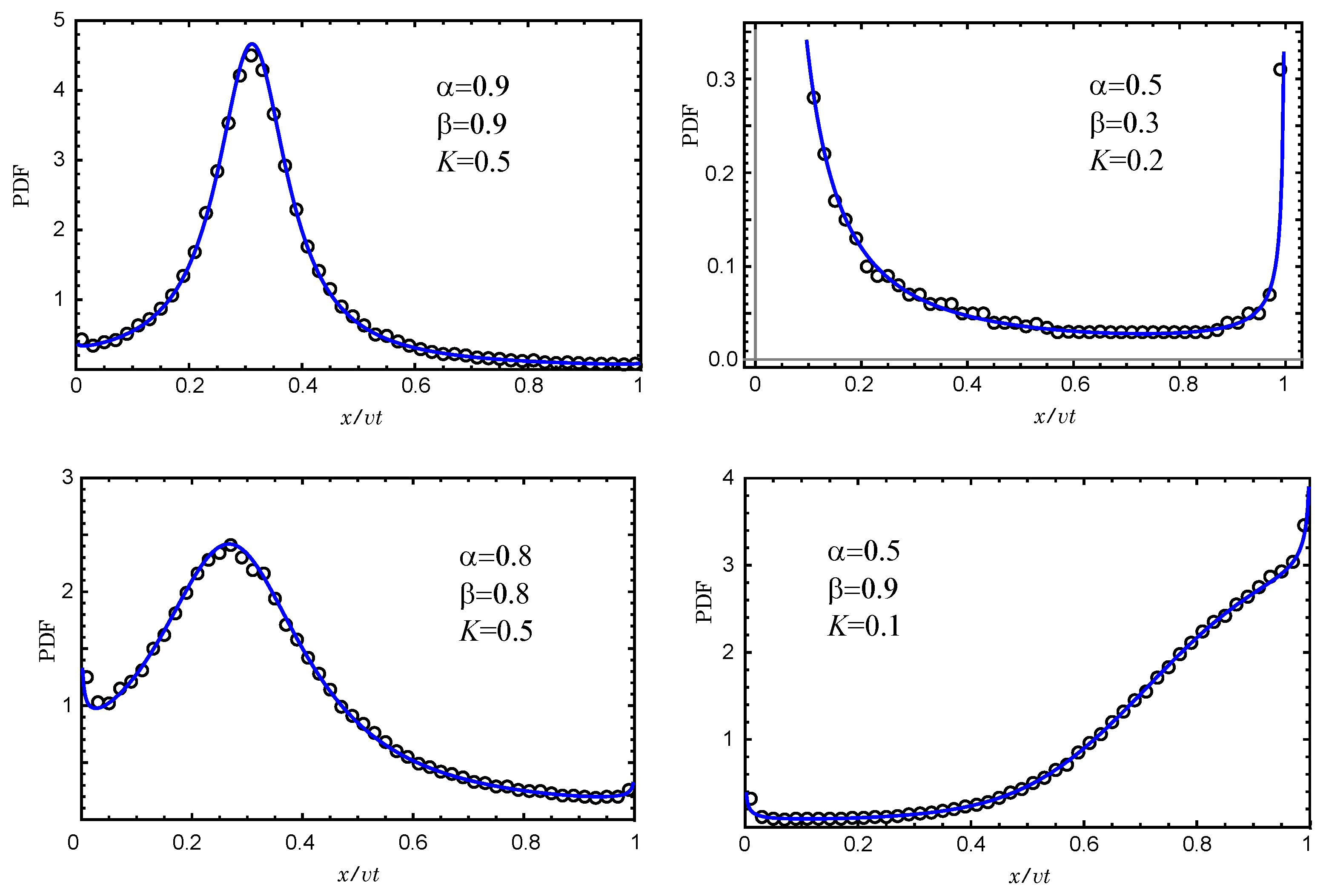
The comparison of these pdfs for different values of $0<\alpha =\beta <1$ and K with the results of the Monte Carlo simulation is shown in Figure 7. Formula (83) perfectly describes the asymptotic distribution densities of a one-sided Lévy walk with trapping. For the simulation of waiting times and path lengths, we use densities in the form of “fractional exponentials” (see, e.g., [16]),

$$\widehat{\psi }\left(s\right)=\frac{1}{1+{\tau }^{\beta }{s}^{\beta }},\widehat{p}\left(k\right)\sim \frac{1}{1+l^{\alpha }{k}^{\alpha }},{\mu }_{\beta }={\tau }^{-\beta },{\mu }_{\alpha }=l^{-\alpha }$$

for which expressions for the Monte Carlo simulation are known [16]:

$$T=\tau |\ln U{|}^{1/\beta }{S}_{\beta },X=l|\ln U{|}^{1/\alpha }{S}_{\alpha }.$$

Here, $S_{\alpha }$ and $S_{\beta }$ are one-sided stable random variables of order $\alpha \in (0,1]$ and $\beta \in (0,1]$.

If $\alpha =\beta$, the fractional stable density is expressed through the elementary function:

$$q^{(\alpha ,\alpha )}\left(x\right)=\frac{sin\pi \alpha }{\pi x(x^{\alpha }+x^{-\alpha }+2cos\pi \alpha )},$$

and the solution takes the form of the Lamperti function:

$$w^{(\alpha ,\alpha )}(\tau ,t)=\frac{sin\pi \alpha }{\pi }\frac{vt{\tau }^{\alpha -1}{\left(t-\tau \right)}^{\alpha -1}}{K{\left(t-\tau \right)}^{2\alpha }+K^{-1}{\tau }^{2\alpha }+2{\left(t-\tau \right)}^{\alpha }{\tau }^{\alpha }cos\pi \alpha }.$$

9. Generalized Cases

In this section, we shortly discuss some generalized cases of one-dimensional random walks, where the obtained solutions can be applied.

9.1. Two-Sided Lévy Walks with Traps

The asymptotic ($t\to \infty$) solution for the pdf of a walking particle coordinate can be written in terms of an integral with the subordinating function

$$p(x,t)={\int }_0^t{p}_1(x,\tau )w(\tau ,t)d\tau .$$

(84)

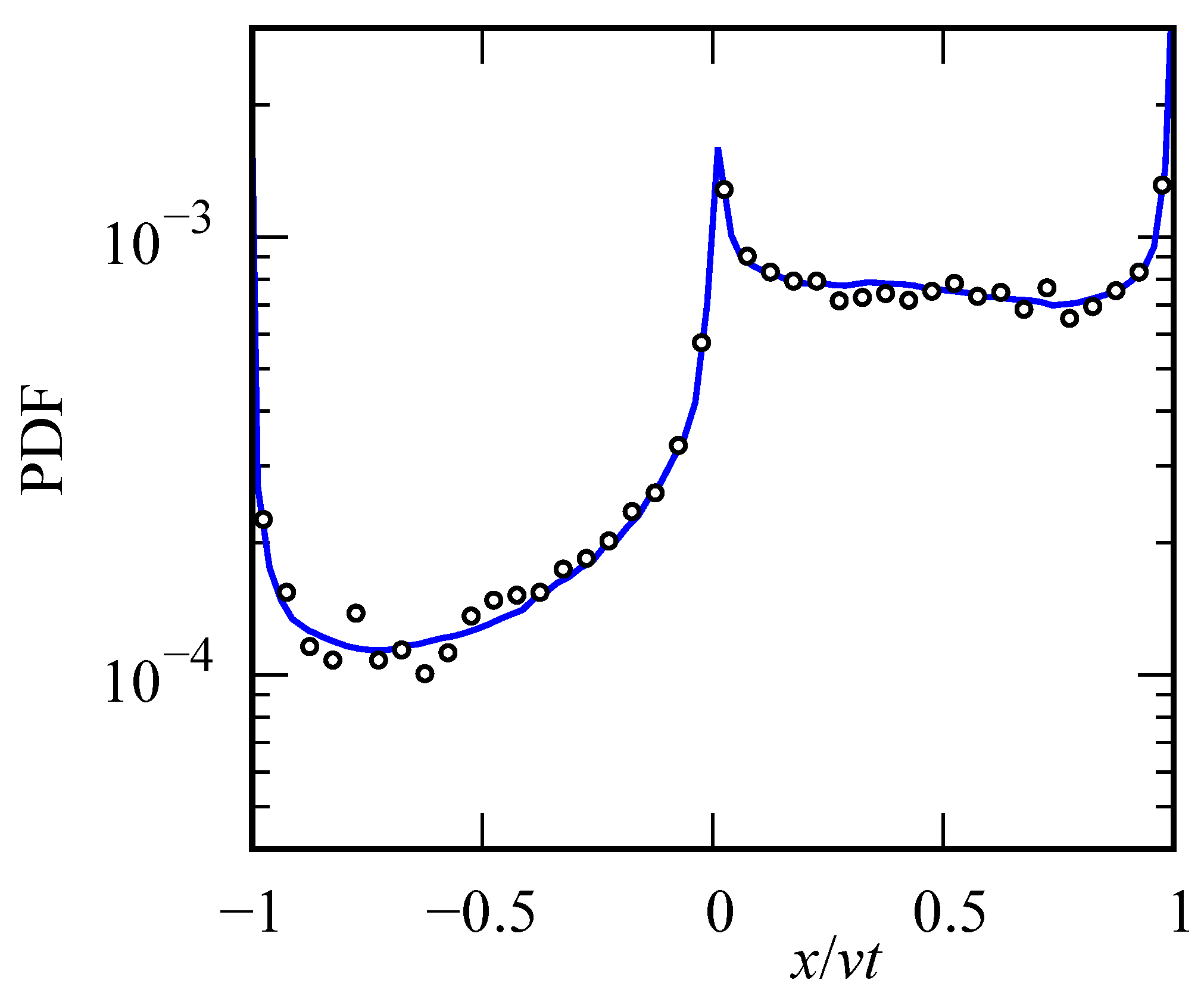
Here, $p_1(x,\tau )$ is the solution for a random walk without traps, and $w(\tau ,t)$ is the distribution density for operational time. For the case of Lévy walks, expressions for $p_1(x,\tau )$ are given in and Section 8 and Section 9. For $w(\tau ,t)$, we can use the asymptotic expression (83) with $\tau$ instead of $x/v$, when the distribution of waiting times and motion times are distributed according to (81) and (82). The comparison of a numerically computed integral (84) with results of the Monte Carlo simulation for the case $\alpha =0.6$, $\beta =0.7$ and asymmetry parameter $\theta =0.5$ is shown in Figure 8. The agreement is satisfactory.

9.2. Asymmetric Fractal Random Walks

We consider the problem of a random walk of a particle along the x axis with a constant speed v and pdf’s of free path lengths $p_{-}\left(x\right)$ and $p_{+}\left(x\right)$ of motion in negative and positive directions, respectively. After each scattering event, the walker continues its motion with probabilities ${\epsilon }_{-}$ and ${\epsilon }_{+}$ in negative and positive directions, respectively. The probability density function $\psi (x,t)$ of the walker coordinate at time t is given by

$$\psi (x,t)=\underset{0}{\overset{t}{\int }}[{\epsilon }_{-}\psi (x+v\tau ,t-\tau )p_{-}\left(v\tau \right)+{\epsilon }_{+}\psi (x-v\tau ,t-\tau )p_{+}\left(v\tau \right)]d\tau$$

$$+{\epsilon }_{-}{P}_{-}\left(vt\right)\delta (x+vt)+{\epsilon }_{+}{P}_{+}\left(vt\right)\delta (x-vt),$$

(85)

where

$$P_{\pm }\left(x\right)=\underset{x}{\overset{+\infty }{\int }}{p}_{\pm }\left(\xi \right)d\xi ,$$

(86)

and

$$p_{\pm }\left(x\right)\propto x^{-1-{\alpha }_{\pm }},x\to +\infty ,0<{\alpha }_{\pm }<1.$$

(87)

Introducing a new variable $\eta =\frac{x+vt}{2v}$, we can rewrite Equation (85) in the form

$$\begin{array}{c}\hfill \psi (\eta ,t)={\epsilon }_{-}\underset{0}{\overset{t}{\int }}\psi (\eta ,t-z)p_{-}\left(z\right)dz+{\epsilon }_{+}\underset{0}{\overset{\eta }{\int }}\psi (\eta -z,t-z)p_{+}\left(z\right)dz\\ \hfill +\frac{{\epsilon }_{-}}{2v}{P}_{-}\left(t\right)\delta \left(\eta \right)+\frac{{\epsilon }_{+}}{2v}{P}_{+}\left(t\right)\delta (t-\eta )\end{array}$$

(88)

Applying a Laplace transformation on t, we arrive at

$$\begin{array}{c}\hfill \psi (\eta ,s)={\epsilon }_{+}\underset{0}{\overset{\eta }{\int }}\psi (\eta -z,s)e^{-zs}{p}_{+}\left(z\right)dz+{\epsilon }_{-}\psi (\eta ,s)p_{-}\left(s\right)+\frac{{\epsilon }_{-}}{2v}{P}_{-}\left(s\right)\delta \left(\eta \right)+\frac{{\epsilon }_{+}}{2v}{P}_{+}\left(\eta \right)e^{-\eta s}\end{array}$$

(89)

After the Laplace transformation on $\eta$, we have

$$\begin{array}{c}\hfill \psi (\lambda ,s)={\epsilon }_{+}\psi (\lambda ,s)p_{+}(\lambda +s)+{\epsilon }_{-}\psi (\lambda ,s)p_{-}\left(s\right)+\frac{{\epsilon }_{-}}{2v}{P}_{-}\left(s\right)+\frac{{\epsilon }_{+}}{2v}{P}_{+}(\lambda +s).\end{array}$$

(90)

The latter equation gives

$$\begin{array}{c}\hfill \widehat{\psi }(\lambda ,s)=\frac{1}{2v}\frac{{\epsilon }_{-}{P}_{-}\left(s\right)+{\epsilon }_{+}{P}_{+}(s+\lambda )}{1-{\epsilon }_{-}{p}_{-}\left(s\right)-{\epsilon }_{+}{p}_{+}(s+\lambda )}\end{array}$$

(91)

10. Conclusions

One-dimensional non-Markovian random walk models with a finite velocity between scattering events have been considered. The exact solution is expressed in terms of multiple convolutions of path-distributions assumed to be different for positive and negative directions of the walk axis. Several particular cases have been considered when the convolutions can be expressed in explicit form. A solution of the fractional telegraph equation has been investigated, and asymptotic behavior of its solution has been provided.

The results obtained belong to the new direction of the kinetics called the non-local transport theory [19,20,21,22]. This theory reveals the high efficiency in problems related to transport in porous materials [23,24], turbulent systems [22], blinking fluorescence of single colloidal nanocrystals [17,25,26], cold atoms in optical lattices [27], protein random walk along DNA [28], solar cosmic ray transport [29,30,31].

References

1. Fock, V.A. Solution of a problem of the theory of diffusion by the method of finite dif-ferences and its application to the diffusion of light. Proc. State Opt. Inst. 1926, 4, 1. (In Russian) [Google Scholar]
2. Davydov, B.I. Fokker-Planck equation and Maxwellian distribution relaxation time. Dokl. Akad. Nauk SSSR 1934, 2, 212. (In Russian) [Google Scholar]
3. Li, T.; Kheifets, S.; Medellin, D.; Raizen, M.G. Measurement of the instantaneous velocity of a Brownian particle. Science 2010, 328, 1673–1675. [Google Scholar] [CrossRef] [Green Version]
4. Monin, A.S. Smoke propagation in the surface layer of the atmosphere. Adv. Geophys. 1959, 6, 331–343. [Google Scholar]
5. Kolmogorov, A.N. On the analytic methods of probability theory. Uspekhi-Temat. Nauk. 1938, 5, 5–41. (In Russian) [Google Scholar]
6. Uchaikin, V.V. Fractional phenomenology of cosmic ray anomalous diffusion. Phys.-Uspekhi 2013, 56, 1074. [Google Scholar] [CrossRef]
7. Feller, W. An Introduction to Probability Theory and Its Applications; John Wiley & Sons: Hoboken, NJ, USA, 2008; Volume 2. [Google Scholar]
8. Bell, W.W. Special Functions for Scientists and Engineers; Dover Publications: New York, NY, USA, 2004. [Google Scholar]
9. Zolotarev, V.M. One-dimensional stable distributions; American Mathematical Society: Providence, RI, USA, 1986. [Google Scholar]
10. Shlesinger, M.F.; Klafter, J.; West, B.J. Lévy walks with applications to turbulence and chaos. Phys. Stat. Mech. Its Appl. 1986, 140, 212–218. [Google Scholar] [CrossRef]
11. Sokolov, I.M.; Metzler, R. Towards deterministic equations for Lévy walks: The fractional material derivative. Phys. Rev. 2003, 67, 010101. [Google Scholar] [CrossRef] [Green Version]
12. Uchaikin, V.V.; Sibatov, R.T. One-dimensional fractal walk at a finite free motion velocity. Tech. Phys. Lett. 2004, 30, 316–318. [Google Scholar] [CrossRef]
13. Pagnini, G.; Vitali, S. Should I stay or should I go? Zero-size jumps in random walks for Lévy flights. Fract. Calc. Appl. Anal. 2021, 24, 137–167. [Google Scholar] [CrossRef]
14. Lamperti, J. An occupation time theorem for a class of stochastic processes. Trans. Am. Math. Soc. 1958, 88, 380–387. [Google Scholar] [CrossRef]
15. Bel, G.; Barkai, E. Random walk to a nonergodic equilibrium concept. Phys. Rev. 2006, 73, 016125. [Google Scholar] [CrossRef] [Green Version]
16. Uchaikin, V.V.; Sibatov, R. Fractional Kinetics in Solids: Anomalous Charge Transport in Semiconductors, Dielectrics, and Nanosystems; World Scientific: Singapore, 2013. [Google Scholar]
17. Sibatov, R.T.; Uchaikin, V.V. Statistics of photocounts of blinking fluorescence of quantum dots. Opt. Spectrosc. 2010, 108, 761–767. [Google Scholar] [CrossRef]
18. Uchaikin, V.V. Fractional Derivatives for Physicists and Engineers; Springer: Berlin/Heidelberg, Germany, 2013; Volume 2. [Google Scholar]
19. Callen, J.D.; Kissick, M.W. Evidence and concepts for non-local transport. Plasma Phys. Controll. Fusion 1997, 39, B173. [Google Scholar] [CrossRef]
20. Ida, K.; Shi, Z.; Sun, H.J.; Inagaki, S. Towards an emerging understanding of non-locality phenomena and non-local transport. Nuclear Fusion 2015, 55, 013022. [Google Scholar] [CrossRef]
21. Uchaikin, V.V.; Sibatov, R.T. On propagators of nonlocal relativistic diffusion of galactic cosmic rays. Phys. Part. Nuclei 2018, 49, 120–124. [Google Scholar] [CrossRef]
22. Uchaikin, V.V. Nonlocal Turbulent Diffusion Models. J. Math. Sci. 2021, 253, 573–582. [Google Scholar] [CrossRef]
23. Koch, D.L.; Brady, J.F. A non-local description of advection-diffusion with application to dispersion in porous media. J. Fluid Mech. 1987, 180, 387–403. [Google Scholar] [CrossRef] [Green Version]
24. Sibatov, R.T. Fractal generalization of the Scher–Montroll model for anomalous transit-time dispersion in disordered solids. Mathematics 2020, 8, 1991. [Google Scholar] [CrossRef]
25. Stefani, F.D.; Hoogenboom, J.P.; Barkai, E. Beyond quantum jumps: Blinking nanoscale light emitters. Phys. Today 2009, 62, 34–39. [Google Scholar] [CrossRef] [Green Version]
26. Khan, S.; Li, W.; Karedla, N.; Thiart, J. Charge-driven fluorescence blinking in carbon nanodots. The J. Phys. Chem. Lett. 2017, 8, 5751–5757. [Google Scholar] [CrossRef]
27. Marksteiner, S.; Ellinger, K.; Zoller, P. Anomalous diffusion and Lévy walks in optical lattices. Phys. Rev. A 1996, 53, 3409. [Google Scholar] [CrossRef] [Green Version]
28. Gorman, J.; Greene, E.C. Visualizing one-dimensional diffusion of proteins along DNA. Nat. Struct. Mol. Biol. 2008, 15, 768–774. [Google Scholar] [CrossRef]
29. Perri, S.; Zimbardo, G. Superdiffusive transport of electrons accelerated at corotating interaction regions. J. Geophys. Res. Space Phys. 2008, 113, A3. [Google Scholar] [CrossRef]
30. Uchaikin, V.V.; Sibatov, R.T. Fractional Kinetics in Space: Anomalous Transport Models; World Scientific: Singapore, 2017. [Google Scholar]
31. Litvinenko, Y.E.; Effenberger, F. Analytical solutions of a fractional diffusion-advection equation for solar cosmic-ray transport. Astrophys. J. 2014, 796, 125. [Google Scholar] [CrossRef] [Green Version]
Figure 1. (a) The result (52) for exponential distribution of path lengths (only regular parts). On this figure t = 3 , v = 1 . For 1, we chose ε 1 = ε 2 = 1 2 and μ 1 = μ 2 = 1 , for 2, ε 1 = 0.99 , ε 2 = 0.01 , μ 1 = μ 2 = 1 , for 3, ε 1 = ε 2 = 1 2 , μ 1 = 1 , μ 2 = 2 and for 4, ε 1 = 0.99 , ε 2 = 0.01 , μ 1 = 1 , μ 2 = 2 . (b) The result for gamma distribution (only regular parts) for ν 1 = ν 2 = 2 . The other parameters are the same as in (a).
Mathematics 09 01264 g001
Figure 2. Monte Carlo results versus exact solution (only regular part). On this figure t = 3 , v = 1 . (a) Result for exponential distribution with, ε 1 = 0.99 , ε 2 = 0.01 , μ 1 = 1 , μ 2 = 2 . (b) Result for gamma distribution with ν 1 = ν 2 = 2 , μ 1 = μ 2 = 1 and ε 1 = ε 2 = 1 / 2 .
Mathematics 09 01264 g002
Figure 3. (a) The result of numerical computations using (41) and (42) for gamma distribution (a) and Bessel distribution (b) for different parameters. On this picture, v = 1 and t = 3 . The outer columns indicate the fraction of unscattered particles.
Mathematics 09 01264 g003
Figure 4. (a) The result of numerical computations using (41) and (42) for a one-sided stable distribution for different parameters α and a comparison with Monte Carlo simulations for α = 0.7 (b) for different parameters. In this figure, v = 1 and t = 3 .
Mathematics 09 01264 g004
Figure 5. Distribution densities for α = 0.7 and 0.5. Points are the result of a Monte Carlo simulation.
Mathematics 09 01264 g005
Figure 6. Evolution of the reduced solution ( v t < x < v t ) for instantaneous point source and its tendency to the asymptotic Lamperti distribution ( α = 0.75 ).
Mathematics 09 01264 g006
Figure 7. Comparison of solution (83) with the Monte Carlo simulation results. There are no fit parameters.
Mathematics 09 01264 g007
Figure 8. Distribution of particle coordinate x / v t for Lévy walks ( α = 0.6 ) with traps ( β = 0.7 ).
Mathematics 09 01264 g008
Publisher’s Note: MDPI stays neutral with regard to jurisdictional claims in published maps and institutional affiliations.