Bell Polynomial Approach for Time-Inhomogeneous Linear Birth–Death Process with Immigration

Abstract

We considered the time-inhomogeneous linear birth–death processes with immigration. For these processes closed form expressions for the transition probabilities were obtained in terms of the complete Bell polynomials. The conditional mean and the conditional variance were explicitly evaluated. Several time-inhomogeneous processes were studied in detail in view of their potential applications in population growth models and in queuing systems. A time-inhomogeneous linear birth–death processes with finite state-space was also taken into account. Special attention was devoted to the cases of periodic immigration intensity functions that play an important role in the description of the evolution of dynamic systems influenced by seasonal immigration or other regular environmental cycles. Various numerical computations were performed for periodic immigration intensity functions.

1. Introduction

Birth–death processes are continuous-time Markov chains on the state space of non-negative integers, in which only transitions to adjacent states are allowed. These processes have been used as models in populations growth and in queuing systems and in many other fields of both theoretical and applied interest (cf., for instance, Bailey [1], Conolly [2], Feldman [3], Iosifescu and Tautu [4], Medhi [5], Ricciardi [6] and Thieme [7]).

Very often, in growth models, immigration’s effects may occur, due to the circumstance that the population is not isolated. In these cases, it is necessary take into account birth–death processes with a reflecting condition in the zero state (see, for instance, Di Crescenzo et al. [8], Crawford and Suchard [9], Giorno and Nobile [10], Lenin et al. [11] and Tavaré [12]). These processes provide interesting applications in queuing models in which a reflecting boundary must be imposed to describe the number of customers in the system (cf., for instance, Crawford et al. [13], Di Crescenzo et al. [14] and Giorno et al. [15]).

In some instances, birth–death processes have also been studied under the effect of catastrophes of various types, interpretable as failures of the system, that produce transitions from the current state to the zero state from which the process can start again (see, Di Crescenzo et al. [16], Dharmaraja et al. [17], Giorno and Nobile [18], Economou and Fakinos [19] and Kapodistria et al. [20]).

Time-inhomogeneous birth–death processes are frequently used to model a large number of real systems in various applied fields, such as in queuing systems and in population growth (see, for instance, Branson [21], Di Crescenzo et al. [22], Giorno et al. [23], Giveen [24], Zeifman et al. [25] and Satin et al. [26]). In particular, birth–death processes with periodic intensity functions play an important role in the description of the evolution of dynamic systems. For instance, the population growth can be influenced by some kind of periodicity: daily, weekly, seasonal and annual (see, Giorno and Nobile [27]). Moreover, queuing systems may be affected by the existence of peak hours in the day (see, Dong and Whitt [28], Giorno et al. [29] and Whitt [30]). Therefore, to model these real systems we used the time-inhomogeneous stochastic processes to obtain probabilistic and statistical characteristics useful for their description. Some recent studies of time-dependent diffusion have delivered new results regarding anomalous diffusion in living biological cells and complex fluids (cf. Bodrova [31,32]).

In the present paper, we focus on a general linear time-inhomogeneous birth and death process with immigration $\{N\left(t\right),t\ge t_0\}$, with time-varying intensity functions. In the literature, specific cases of time-inhomogeneous processes are considered and, almost always, concern processes with proportional time-varying intensity functions.

In Section 2, for $N\left(t\right)$ we obtain closed form expressions for the generating probability function and for the transition probabilities $p_{j,n}\left(t\right|t_0)$, from an initial state j at time $t_0$ to the state n at time t, in terms of the complete Bell polynomials. The conditional mean and the conditional variance of $N\left(t\right)$ are also explicitly determined. The well-known results for the time-homogeneous birth and death process with immigration are also derived.

In Section 3, we revisit a variety of inhomogeneous immigration-birth–death processes, such as the generalized Polya process and the generalized Polya-death process, by obtaining closed form results for the transition probabilities via our approach based on the complete Bell polynomials. Expressions for conditional mean and conditional variance are also explicitly given.

In Section 4, we take into account a time-inhomogeneous birth–death process with finite state-space, known in the literature as the time-inhomogeneous Prendiville process.

The proofs of propositions are shown in the Appendix A, Appendix B, Appendix C, Appendix D and Appendix E.

Various numerical computations were also performed with MATHEMATICA to analyze the role played from the parameters, by devoting special attention to the case of periodic immigration intensity functions.

2. The Model

Let $\{N\left(t\right),t\ge t_0\}$ be a time-inhomogeneous linear birth–death process with immigration ($NHBDI$) having state-space ${\mathbb{N}}_0$, conditioned to start from $j\in {\mathbb{N}}_0$ at time $t_0$. We assume that $N\left(t\right)$ is regulated from transitions that occur in according to the following scheme:

• $n\to n+1$ with rate ${\lambda }_n\left(t\right)=n\lambda \left(t\right)+\nu \left(t\right)$ for $n=0,1,\dots$,
• $n\to n-1$ with rate ${\mu }_n\left(t\right)=n\mu \left(t\right)$ for $n=1,2,\dots$,

where $\lambda \left(t\right)$, $\mu \left(t\right)$ and $\nu \left(t\right)$ are positive, bounded and continuous functions for $t\ge t_0$ representing birth, death and immigration intensity functions, respectively. We denote by

$$p_{j,n}\left(t\right|t_0)=P\{N\left(t\right)=n|N\left(t_0\right)=j\},j,n\in {\mathbb{N}}_0,t\ge t_0$$

the transition probabilities of $N\left(t\right)$. They satisfy the Kolmogorov forward equations and the related initial condition:

$$\begin{array}{c}\frac{d{p}_{j,0}\left(t\right|t_0)}{dt}=-\nu \left(t\right)p_{j,0}\left(t\right|t_0)+\mu \left(t\right)p_{j,1}\left(t\right|t_0),\hfill \\ \frac{d{p}_{j,n}\left(t\right|t_0)}{dt}=[\lambda \left(t\right)(n-1)+\nu \left(t\right)]p_{j,n-1}\left(t\right|t_0)-\{[\lambda \left(t\right)+\mu \left(t\right)]n+\nu \left(t\right)\}{p}_{j,n}\left(t\right|t_0)\hfill \\ +\mu \left(t\right)(n+1)p_{j,n+1}\left(t\right|t_0),n\in \mathbb{N},\hfill \\ \underset{t\downarrow t_0}{lim}{p}_{j,n}\left(t\right|t_0)={\delta }_{j,n},\hfill \end{array}$$

(1)

where ${\delta }_{j,n}$ is the Kronecker delta function. For $t\ge t_0$ and $0\le z\le 1$, let

$$G_j(z,t)=\sum _{n=0}^{+\infty }{z}^n{p}_{j,n}\left(t\right|t_0)$$

(2)

be the probability generating function of $N\left(t\right)$. Due to (1), $G_j(z,t)$ is solution of

$$\begin{array}{cc}\hfill & \frac{\partial G_j(z,t)}{\partial t}-(z-1)\left[\lambda \left(t\right)z-\mu \left(t\right)\right]\frac{\partial G_j(z,t)}{\partial z}=\nu \left(t\right)(z-1)G_j(z,t),\hfill \\ \hfill & G_j(z,t_0)=z^j.\hfill \end{array}$$

(3)

In the following, for $t\ge t_0$ we denote by

$$\Lambda \left(t\right|t_0)={\int }_{t_0}^t\lambda \left(\tau \right)d\tau ,M\left(t\right|t_0)={\int }_{t_0}^t\mu \left(\tau \right)d\tau$$

(4)

the cumulative birth and death intensity functions, respectively.

Proposition 1.

For $t\ge t_0$ and $j\in {\mathbb{N}}_0$, the probability generating function of the $NHBDI$ process $N\left(t\right)$ is:

$$\begin{array}{ccc}\hfill & \hfill & G_j(z,t)=exp\left\{(z-1){\int }_{t_0}^t\frac{\nu \left(u\right)e^{\Lambda \left(t\right|u)-M(t\left|u\right)}}{1-(z-1)e^{\Lambda \left(t\right|t_0)-M\left(t\right|t_0)}[A\left(t\right|t_0)-A\left(u\right|t_0)]}du\right\}\hfill \\ \hfill & \hfill & \times {\left[\frac{1+(z-1)e^{\Lambda \left(t\right|t_0)-M\left(t\right|t_0)}[1-A\left(t\right|t_0)]}{1-(z-1)e^{\Lambda \left(t\right|t_0)-M\left(t\right|t_0)}A\left(t\right|t_0)}\right]}^j,\hfill \end{array}$$

(5)

where

$$A\left(t\right|t_0)={\int }_{t_0}^t\lambda \left(\tau \right)e^{M\left(\tau \right|t_0)-\Lambda \left(\tau \right|t_0)}d\tau .$$

(6)

Proof. 

The proof is given in Appendix A. □

The expression of the probability generating function (5) allows us to determine the conditional mean and the conditional variance of the $NHBDI$ process $N\left(t\right)$. Indeed, for $t\ge t_0$ and $j\in {\mathbb{N}}_0$ one has:

$$\begin{array}{cc}\hfill & \mathrm{E}\left[N\left(t\right)\right|N\left(t_0\right)=j]=j{e}^{\Lambda \left(t\right|t_0)-M\left(t\right|t_0)}+{\int }_{t_0}^t\nu \left(u\right)e^{\Lambda \left(t\right|u)-M(t\left|u\right)}du,\hfill \\ \hfill & \mathrm{Var}\left[N\left(t\right)\right|N\left(t_0\right)=j]=j{e}^{\Lambda \left(t\right|t_0)-M\left(t\right|t_0)}\left\{1-e^{\Lambda \left(t\right|t_0)-M\left(t\right|t_0)}+2e^{\Lambda \left(t\right|t_0)-M\left(t\right|t_0)}A\left(t\right|t_0)\right\}\hfill \\ \hfill & +{\int }_{t_0}^t\nu \left(u\right)e^{\Lambda \left(t\right|u)-M(t\left|u\right)}du+2e^{\Lambda \left(t\right|t_0)-M\left(t\right|t_0)}{\int }_{t_0}^t\nu \left(u\right)e^{\Lambda \left(t\right|u)-M(t\left|u\right)}\left[A\left(t\right|t_0)-A\left(u\right|t_0)\right]du.\hfill \end{array}$$

(7)

From (5), for $t\ge t_0$ we note that

$$G_j(z,t)=\left\{\begin{array}{cc}{G}_0(z,t),\hfill & j=0,\hfill \\ G_0(z,t)H_j(z,t),\hfill & j\in \mathbb{N},\hfill \end{array}\right.$$

(8)

where $G_0(z,t)$ is the probability generating function of the process $N\left(t\right)$ for $j=0$ and where

$$H_j(z,t)={\left[\frac{1+(z-1)e^{\Lambda \left(t\right|t_0)-M\left(t\right|t_0)}[1-A\left(t\right|t_0)]}{1-(z-1)e^{\Lambda \left(t\right|t_0)-M\left(t\right|t_0)}A\left(t\right|t_0)}\right]}^j,j\in \mathbb{N}$$

(9)

is the probability generating function of a linear time-inhomogeneous birth–death ($NHBD$) process $\{M\left(t\right),t\ge t_0\}$, whose intensity functions are ${\lambda }_n\left(t\right)=n\lambda \left(t\right)$ and ${\mu }_n\left(t\right)=n\mu \left(t\right)$ for $n\in \mathbb{N}$.

Therefore, to determine the probabilities $p_{j,n}\left(t\right|t_0)$ for $j,n\in {\mathbb{N}}_0$ of the $NHBDI$ process $N\left(t\right)$, we proceed as follows:

(1)

we determine the transition probabilities $p_{0,n}\left(t\right|t_0)$ for $n\in {\mathbb{N}}_0$ and $t\ge t_0$;

(2)

we calculate the probabilities $p_{j,n}\left(t\right|t_0)$ as a convolution between $p_{0n}\left(t\right|t_0)$ and the transition probabilities of the process $M\left(t\right)$ for $j\in \mathbb{N}$, $n\in {\mathbb{N}}_0$ and $t\ge t_0$.

We now recall some results on the $NHBD$ process $M\left(t\right)$, which will be useful in the following. Denoting by

$$f_{j,n}\left(t\right|t_0)=P\{M\left(t\right)=n|M\left(t_0\right)=j\},j\in \mathbb{N},n\in {\mathbb{N}}_0,t\ge t_0$$

the transition probabilities of $M\left(t\right)$, by expanding (9) in powers series of z, for $t\ge t_0$ one obtains (cf. Bailey [1]):

$$\begin{array}{c}{f}_{j,n}\left(t\right|t_0)=\sum _{r=0}^{min(n,j)}\left(\genfrac{}{}{0pt}{}{j}{r}\right)\left(\genfrac{}{}{0pt}{}{j+n-r-1}{j-1}\right){\left[\alpha \left(t\right|t_0)\right]}^{j-r}{\left[\beta \left(t\right|t_0)\right]}^{n-r}{[1-\alpha \left(t\right|t_0)-\beta \left(t\right|t_0)]}^r,j\in \mathbb{N},n\in {\mathbb{N}}_0,\hfill \end{array}$$

(10)

where we have set:

$$\alpha \left(t\right|t_0)=\frac{1+[A\left(t\right|t_0)-1]e^{\Lambda \left(t\right|t_0)-M\left(t\right|t_0)}}{1+A\left(t\right|t_0)e^{\Lambda \left(t\right|t_0)-M\left(t\right|t_0)}},\beta \left(t\right|t_0)=\frac{A\left(t\right|t_0)e^{\Lambda \left(t\right|t_0)-M\left(t\right|t_0)}}{1+A\left(t\right|t_0)e^{\Lambda \left(t\right|t_0)-M\left(t\right|t_0)}}·$$

(11)

2.1. Determination of the Transition Probabilities Starting from the Zero State

We obtain the transition probabilities for the $NHBDI$ process $N\left(t\right)$ when the process moves starting from the zero state.

Proposition 2.

For $t\ge t_0$ and $j=0$, the transition probabilities of the $NHBDI$ process $N\left(t\right)$ are:

$$p_{0,n}\left(t\right|t_0)=exp\left\{-{\int }_{t_0}^t\frac{\nu \left(u\right)e^{\Lambda \left(t\right|u)-M(t\left|u\right)}}{1+e^{\Lambda \left(t\right|t_o)-M\left(t\right|t_0)}[A\left(t\right|t_0)-A\left(u\right|t_0)]}du\right\}\frac{B_n(d_1,d_2,\dots ,d_n)}{n!},n\in {\mathbb{N}}_0,$$

(12)

where $A\left(t\right|t_0)$ is given in (6) and $B_n(d_1,d_2,\cdots ,d_n)$ are the complete Bell polynomials recurrently defined as follows:

$$B_0=1,B_{n+1}(d_1,d_2,\dots ,d_{n+1})=\sum _{i=0}^n\left(\genfrac{}{}{0pt}{}{n}{i}\right)B_{n-i}(d_1,d_2,\dots ,d_{n-i})d_{i+1},n\in {\mathbb{N}}_0,$$

(13)

with

$$d_r\equiv d_r\left(t\right|t_0)=r!e^{(r-1)[\Lambda \left(t\right|t_0)-M\left(t\right|t_0)]}{\int }_{t_0}^t\frac{\nu \left(u\right)e^{\Lambda \left(t\right|u)-M(t\left|u\right)}{[A\left(t\right|t_0)-A\left(u\right|t_0)]}^{r-1}}{{\left\{1+e^{\Lambda \left(t\right|t_0)-M\left(t\right|t_0)}[A\left(t\right|t_0)-A\left(u\right|t_0)]\right\}}^{r+1}}du,r\in \mathbb{N}.$$

(14)

Proof. 

The proof is given in Appendix B. □

Remark 1.

For the $NHBDI$ process $N\left(t\right)$, one has:

$$\begin{array}{cc}\hfill & p_{0,0}\left(t\right|t_0)=e^{-R_1\left(t\right|t_0)},\hfill \\ \hfill & p_{0,1}\left(t\right|t_0)=p_{0,0}\left(t\right|t_0)R_2\left(t\right|t_0),\hfill \\ \hfill & p_{0,2}\left(t\right|t_0)=p_{0,0}\left(t\right|t_0)\left[\frac{1}{2}{R}_2^2\left(t\right|t_0)+e^{\Lambda \left(t\right|t_0)-M\left(t\right|t_0)}{S}_3\left(t\right|t_0)\right],\hfill \end{array}$$

(15)

where we have set:

$$\begin{array}{c}{R}_k\left(t\right|t_0)={\int }_{t_0}^t\frac{\nu \left(u\right)e^{\Lambda \left(t\right|u)-M(t\left|u\right)]}}{{\left\{1+e^{\Lambda \left(t\right|t_0)-M\left(t\right|t_0)}[A\left(t\right|t_0)-A\left(u\right|t_0)]\right\}}^k}du,k=1,2,\dots ,\hfill \\ \hfill \\ S_k\left(t\right|t_0)={\int }_{t_0}^t\frac{\nu \left(u\right)e^{\Lambda \left(t\right|u)-M(t\left|u\right)}[A\left(t\right|t_0)-A\left(u\right|t_0)]}{{\left\{1+e^{\Lambda \left(t\right|t_0)-M\left(t\right|t_0)}[A\left(t\right|t_0)-A\left(u\right|t_0)]\right\}}^k}du,k=1,2,\dots ,\hfill \end{array}$$

(16)

with $A\left(t\right|t_0)$ given in (6).

Proof. 

It follows from (12) by noting that from (13) one has $B_0=1$, $B_1\left(d_1\right)=d_1$ and $B_2(d_1,d_2)=d_1^2+d_2$, with $d_r$ given in (14). □

2.2. Determination of the Transition Probabilities Starting from $j\in \mathbb{N}$

We determine the closed form expressions for the transition probabilities $p_{j,n}\left(t\right|t_0)$ of the $NHBDI$ process $N\left(t\right)$ when $j\in \mathbb{N}$ and $n\in {\mathbb{N}}_0$.

Proposition 3.

For $t\ge t_0$ and $j\in \mathbb{N}$, the transition probabilities of the $NHBDI$ process $N\left(t\right)$ are:

$$\begin{array}{c}{p}_{j,n}\left(t\right|t_0)=exp\left\{-{\int }_{t_0}^t\frac{\nu \left(u\right)e^{\Lambda \left(t\right|u)-M(t\left|u\right)}}{1+e^{\Lambda \left(t\right|t_0)-M\left(t\right|t_0)}[A\left(t\right|t_0)-A\left(u\right|t_0)]}du\right\}\hfill \\ \times \sum _{k=0}^n\frac{B_k(d_1,d_2,\dots d_k)}{k!}\sum _{r=0}^{min(n-k,j)}\left(\genfrac{}{}{0pt}{}{j}{r}\right)\left(\genfrac{}{}{0pt}{}{j+n-k-r-1}{j-1}\right)\hfill \\ \times {\left[\alpha \left(t\right|t_0)\right]}^{j-r}{\left[\beta \left(t\right|t_0)\right]}^{n-k-r}{\left[1-\alpha \left(t\right|t_0)-\beta \left(t\right|t_0)\right]}^r,n\in {\mathbb{N}}_0,\hfill \end{array}$$

(17)

with $\alpha \left(t\right|t_0)$, $\beta \left(t\right|t_0)$ defined in (11).

Proof. 

The proof is given in Appendix C. □

Remark 2.

For the $NHBDI$ process $N\left(t\right)$, when $j\in \mathbb{N}$ one has:

$$\begin{array}{c}{p}_{j,0}\left(t\right|t_0)=e^{-R_1\left(t\right|t_0)}{\left[\alpha \left(t\right|t_0)\right]}^j,\hfill \\ p_{j,1}\left(t\right|t_0)=e^{-R_1\left(t\right|t_0)}{\left[\alpha \left(t\right|t_0)\right]}^{j-1}\left\{\alpha \left(t\right|t_0)R_2\left(t\right|t_0)+\frac{j{e}^{\Lambda \left(t\right|t_0)-M\left(t\right|t_0)}}{\{1+e^{\Lambda \left(t\right|t_0)-M\left(t\right|t_0)}A\left(t\right|t_0){\}}^2}\right\},\hfill \\ p_{j,2}\left(t\right|t_0)=e^{-R_1\left(t\right|t_0)}{\left[\alpha \left(t\right|t_0)\right]}^{j-2}\{\frac{1}{2}{\left[\alpha \left(t\right|t_0)R_2\left(t\right|t_0)\right]}^2+{\left[\alpha \left(t\right|t_0)\right]}^2{e}^{\Lambda \left(t\right|t_0)-M\left(t\right|t_0)}{S}_3\left(t\right|t_0)\hfill \\ +\frac{j\alpha \left(t\right|t_0)e^{\Lambda \left(t\right|t_0)-M\left(t\right|t_0)}}{\{1+e^{\Lambda \left(t\right|t_0)-M\left(t\right|t_0)}A\left(t\right|t_0){\}}^2}{R}_2\left(t\right|t_0)+\frac{j(j-1)e^{2[\Lambda \left(t\right|t_0)-M\left(t\right|t_0)]}}{2\{1+e^{\Lambda \left(t\right|t_0)-M\left(t\right|t_0)}A\left(t\right|t_0){\}}^4}\hfill \\ +\frac{j\alpha \left(t\right|t_0)e^{2[\Lambda \left(t\right|t_0)-M\left(t\right|t_0)]}A\left(t\right|t_0)}{\{1+e^{\Lambda \left(t\right|t_0)-M\left(t\right|t_0)}A\left(t\right|t_0){\}}^3}\},\hfill \end{array}$$

where $R_k\left(t\right|t_0)$ and $S_k\left(t\right|t_0)$ are defined in (16), with $A\left(t\right|t_0)$ and $\alpha \left(t\right|t_0)$ given in (6) and (11), respectively.

Proof. 

It follows from (17) recalling (14). □

2.3. Time-Homogeneous Case

We obtain the well-known expressions of the transition probabilities of the time-homogeneous linear birth–death process with immigration ($HBDI$) via Propositions 2 and 3 (cf., for instance, Karlin and McGregor [33]). To this aim, we assume $\lambda \left(t\right)=\lambda$, $\mu \left(t\right)=\mu$, $\nu \left(t\right)=\nu$, with $\lambda$, $\mu$ and $\nu$ positive real numbers. Therefore, from (4), (6) and (11) we have:

$$\Lambda \left(t\right|t_0)=\lambda (t-t_0),M\left(t\right|t_0)=\mu (t-t_0),A\left(t\right|t_0)=\left\{\begin{array}{cc}\lambda (t-t_0),\hfill & \lambda =\mu ,\hfill \\ {\displaystyle \frac{\lambda }{\mu -\lambda }\left[e^{(\mu -\lambda )(t-t_0)}-1\right],}\hfill & \lambda \ne \mu \hfill \end{array}\right.$$

(18)

and $\alpha \left(t\right|t_0)=\mu \varrho \left(t\right|t_0)$, $\beta \left(t\right|t_0)=\lambda \varrho \left(t\right|t_0)$ with

$$\varrho \left(t\right|t_0)=\left\{\begin{array}{cc}{\displaystyle \frac{t-t_0}{1+\lambda (t-t_0)},}\hfill & \lambda =\mu ,\hfill \\ {\displaystyle \frac{e^{(\lambda -\mu )(t-t_0)}-1}{\lambda e^{(\lambda -\mu )(t-t_0)}-\mu },}\hfill & \lambda \ne \mu \hfill \end{array}\right.$$

(19)

Moreover, for the $HBDI$ process from (14) it follows that $d_r=(r-1)!\frac{\nu }{\lambda }{\left[\beta \left(t\right|t_0)\right]}^r$ for $r\in \mathbb{N}$. Then, from (13) we obtain $B_n(d_1,d_2,\dots ,d_n)={\left(\frac{\nu }{\lambda }\right)}_n{\left[\beta \left(t\right|t_0)\right]}^n$, where ${\left(\gamma \right)}_n$ denotes the Pochhammer symbol, which is defined as ${\left(\gamma \right)}_0=1$ and ${\left(\gamma \right)}_n=\gamma (\gamma +1)\cdots (\gamma +n-1)$ for $n=1,2,\dots$ Therefore, for $\lambda \ne \mu$, from (12) and (17) for $t\ge t_0$ one has:

$$\begin{array}{c}{p}_{0,n}\left(t\right|t_0)={\left[\frac{\lambda -\mu }{\lambda e^{(\lambda -\mu )(t-t_0)}-\mu }\right]}^{\nu /\lambda }\frac{1}{n!}{\left(\frac{\nu }{\lambda }\right)}_n{\left[\lambda \varrho \left(t\right|t_0)\right]}^n,n\in {\mathbb{N}}_0,\hfill \\ \hfill \\ p_{j,n}\left(t\right|t_0)={\left[\frac{\lambda -\mu }{\lambda e^{(\lambda -\mu )(t-t_0)}-\mu }\right]}^{\nu /\lambda }\sum _{r=0}^{min(j,n)}\left(\genfrac{}{}{0pt}{}{j}{r}\right)\frac{1}{(n-r)!}{\left(j+\frac{\nu }{\lambda }\right)}_{n-r}{\left[\mu \varrho \left(t\right|t_0)\right]}^{j-r}{\left[\lambda \varrho \left(t\right|t_0)\right]}^{n-r}\hfill \\ \times {[1-(\lambda +\mu )\varrho \left(t\right|t_0)]}^r,j\in \mathbb{N},n\in {\mathbb{N}}_0.\hfill \end{array}$$

(20)

Similarly, for $\lambda =\mu$ and $t\ge t_0$ from (12) and (17) one obtains:

$$\begin{array}{c}{p}_{0,n}\left(t\right|t_0)={\left[\frac{1}{1+\lambda (t-t_0)}\right]}^{\nu /\lambda }\frac{1}{n!}{\left(\frac{\nu }{\lambda }\right)}_n{\left[\frac{\lambda (t-t_0)}{1+\lambda (t-t_0)}\right]}^n,n\in {\mathbb{N}}_0,\hfill \\ \hfill \\ p_{j,n}\left(t\right|t_0)={\left[\frac{1}{1+\lambda (t-t_0)}\right]}^{\nu /\lambda }\sum _{r=0}^{min(j,n)}\left(\genfrac{}{}{0pt}{}{j}{r}\right)\frac{1}{(n-r)!}{\left(j+\frac{\nu }{\lambda }\right)}_{n-r}{\left[\frac{1-\lambda (t-t_0)}{\lambda (t-t_0)}\right]}^r{\left[\frac{\lambda (t-t_0)}{1+\lambda (t-t_0)}\right]}^{j+n-r},\hfill \\ j\in \mathbb{N},n\in {\mathbb{N}}_0.\hfill \end{array}$$

(21)

Expressions (20) and (21) are in agreement with the expressions given in Bayley [1]. Making use of (18) and (19) in (7), for $j\in {\mathbb{N}}_0$ and $t\ge t_0$ one has (cf., for instance, Ricciardi [6]):

$$\begin{array}{c}\mathrm{E}\left[N\left(t\right)\right|N\left(t_0\right)=j]=\left\{\begin{array}{cc}{\displaystyle j+\nu (t-t_0),}\hfill & \lambda =\mu ,\hfill \\ {\displaystyle j{e}^{(\lambda -\mu )(t-t_0)}-\frac{\nu }{\lambda -\mu }\left[e^{(\lambda -\mu )(t-t_0)}-1\right],}\hfill & \lambda \ne \mu ,\hfill \end{array}\right.\hfill \\ \hfill \\ \mathrm{Var}\left[N\left(t\right)\right|N\left(t_0\right)=j]=\left\{\begin{array}{cc}2j\lambda (t-t_0)+\nu (t-t_0)[1+\lambda (t-t_0)],\hfill & \lambda =\mu ,\hfill \\ {\displaystyle \left[e^{(\lambda -\mu )(t-t_0)}-1\right]\left\{\frac{j(\lambda +\mu )}{\lambda -\mu }{e}^{(\lambda -\mu )(t-t_0)}+\frac{\nu \left[\lambda e^{(\lambda -\mu )(t-t_0)}-\mu \right]}{{(\lambda -\mu )}^2}\right\},}\hfill & \lambda \ne \mu .\hfill \end{array}\right.\hfill \end{array}$$

(22)

We note that as $\lambda \ge \mu$ and $\nu >0$, the $HBDI$ process does not admit a limit behavior. Moreover, when $\lambda >\mu$, the mean of population size grows exponentially for large t with rate $\lambda -\mu$, whereas, for $\lambda =\mu$ the mean of population grows linearly with rate $\nu$. Instead, when $\lambda <\mu$, the $HBDI$ process exhibits a steady-state behavior. Therefore, for $\lambda <\mu$ and $\nu >0$ from (20) one has:

$$q_n=\underset{t\to +\infty }{lim}{p}_{j,n}\left(t\right|t_0)=\frac{1}{n!}{\left(\frac{\nu }{\lambda }\right)}_n{\left(1-\frac{\lambda }{\mu }\right)}^{\nu /\lambda }{\left(\frac{\lambda }{\mu }\right)}^n,n\in {\mathbb{N}}_0.$$

(23)

Moreover, from (22) for $\lambda <\mu$ and $\nu >0$ one obtains the asymptotic mean and variance:

$$\mathrm{E}\left(N\right)=\underset{t\to +\infty }{lim}\mathrm{E}\left[N\left(t\right)\right|N\left(t_0\right)=j]=\frac{\nu }{\mu -\lambda },\mathrm{Var}\left(N\right)=\underset{t\to +\infty }{lim}\mathrm{Var}\left[N\left(t\right)\right|N\left(t_0\right)=j]=\frac{\nu \mu }{{(\mu -\lambda )}^2}·$$

(24)

Example 1.

We consider the $NHBDI$ process $N\left(t\right)$, with $t_0=0$, characterized by ${\lambda }_n\left(t\right)=\lambda n+\nu \left(t\right)$ and ${\mu }_n\left(t\right)=\mu n$, with $\lambda >0$ and $\mu >0$, subject to periodic immigration phenomena that occur with intensity function:

$$\nu \left(t\right)=\nu \left[1+asin\left(\frac{2\pi t}{Q}\right)\right],t\ge 0,$$

(25)

where $\nu >0$ is the average of the periodic function $\nu \left(t\right)$ of period Q, a is the amplitude of the oscillations, with $0\le a<1$.

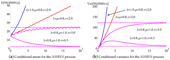
In Figure 1, the conditional mean and the conditional variance, given in (7), of the $NHBDI$ process with constant birth–death rates and periodic immigration intensity function (25) are plotted as function of t for $j=15$, $a=0.9$, $Q=1.0$ and some choices of $\lambda ,\mu$ and ν. The dashed lines indicate the asymptotic mean $E\left(N\right)$ and the asymptotic variance $\mathrm{Var}\left(N\right)$, given in (24), related to $HBDI$ process in the case $\lambda <\mu$ and $\nu >0$.

Figure 1. For the time-inhomogeneous linear birth–death process with immigration ($NHBDI$) having ${\lambda }_n\left(t\right)=\lambda n+\nu \left(t\right)$ and ${\mu }_n\left(t\right)=\mu n$, with $\nu \left(t\right)$ given in (25), the conditional mean and the conditional variance (7) are plotted as function of t for $j=15$, $a=0.9$, $Q=1.0$ and for some choices of $\lambda ,\mu ,\nu$. The dashed lines indicate the asymptotic mean and the asymptotic variance of the $HBDI$ process, given in (24).

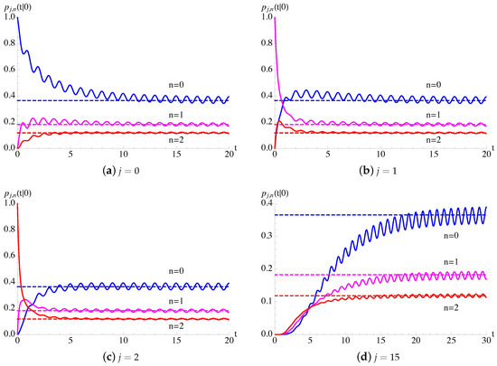
In Figure 2, making use of Remarks 1 and 2, the transition probabilities $p_{j,n}\left(t\right|0)$ are plotted as function of t for $j=0,1,2,15$ and $n=0,1,2$ for some fixed choices of parameters. Since $\lambda <\mu$ and $\nu >0$, we note that the transition probabilities admit a periodic asymptotic behavior, strongly influenced by $\nu \left(t\right)$. Moreover, the asymptotic behavior of $p_{j,n}\left(t\right|0)$ oscillate around the asymptotic probabilities $q_n$, given in (23), of the $HBDI$ process.

Figure 2. For the $NHBDI$ process of Figure 1, the probabilities $p_{j,n}\left(t\right|0)$ are plotted as function of t for $\lambda =0.8$, $\mu =1.0$, $\nu =0.5$, $a=0.9$, $Q=1.0$ with $n=0,1,2$. The dashed lines indicate the asymptotic probabilities $q_0$, $q_1$, $q_2$, given in (23), related to $HBDI$ process.

3. Special Discrete Processes

We derive the expressions for the transition probabilities for some known and not known processes making use of the general results obtained in Section 2. We consider the processes indicated in Table 1.

Table 1. Special time-inhomogeneous linear discrete processes conditioned to start from the state j.

Name	Abbreviation	Intensity Functions
Time-inhomogeneous Poisson process	$NHP$	${\lambda }_n\left(t\right)=\nu \left(t\right)$, $n=j,j+1,\dots ;j\in {\mathbb{N}}_0$
Time-inhomogeneous birth process	$NHB$	${\lambda }_n\left(t\right)=n\lambda \left(t\right)$, $n=j,j+1,\dots ;j\in \mathbb{N}$
Time-inhomogeneous death process	$NHD$	${\mu }_n\left(t\right)=n\mu \left(t\right)$, $n=0,1,\dots ,j;j\in \mathbb{N}$
Time-inhomogeneous birth–death process	$NHBD$	$\begin{array}{c}{\lambda }_n\left(t\right)=n\lambda \left(t\right),n\in \mathbb{N},\hfill \\ {\mu }_n\left(t\right)=n\mu \left(t\right),n\in \mathbb{N};j\in \mathbb{N}\hfill \end{array}$
Time-inhomogeneous death process with immigration	$NHDI$	$\begin{array}{c}{\lambda }_n\left(t\right)=\nu \left(t\right),n\in {\mathbb{N}}_0,\hfill \\ {\mu }_n\left(t\right)=n\mu \left(t\right),n\in \mathbb{N};j\in {\mathbb{N}}_0\hfill \end{array}$
Time-inhomogeneous birth process with immigration	$NHBI$	${\lambda }_n\left(t\right)=\lambda \left(t\right)n+\nu \left(t\right),n=j,j+1,\dots ;j\in {\mathbb{N}}_0$
Generalized Polya process	$GPy$	${\lambda }_n\left(t\right)=\lambda \left(t\right)(n+\nu ),n=j,j+1,\dots ;j\in {\mathbb{N}}_0$
Generalized Polya-death process	$GPyD$	$\begin{array}{c}{\lambda }_n\left(t\right)=\lambda \left(t\right)(n+\nu ),n\in {\mathbb{N}}_0,\hfill \\ {\mu }_n\left(t\right)=n\mu \left(t\right),n\in \mathbb{N};j\in {\mathbb{N}}_0\hfill \end{array}$

3.1. Time-Inhomogeneous Poisson Process

We consider the time-inhomogeneous Poisson ($NHP$) process having state-space $\{j,j+1,\dots \}$, conditioned to start from $j\in {\mathbb{N}}_0$ at time $t_0$. We assume that the birth intensity function is ${\lambda }_n\left(t\right)=\nu \left(t\right)$ for $n=j,j+1,\dots$, with $\nu \left(t\right)$ positive, bounded and continuous function for $t\ge t_0$. Many applications of the NHP process can be found in reliability growth models, in risk analysis, in financial problems and in queuing models. For instance, in queuing systems the NHP process is often used to describe the arrival process to a queue in which the come of customers varies according to the time of day (cf., for instance, Medhi [5], Konno [34]).

In the general $NHBDI$ process, we set $\lambda \left(t\right)=\mu \left(t\right)=0$ and ${\lambda }_n\left(t\right)=\nu \left(t\right)$ for $n=j,j+1,\dots$, so that from (4) and (6) one has $\Lambda \left(t\right|t_0)=M\left(t\right|t_0)=A\left(t\right|t_0)=0$. Hence, from (5), we obtain the well-known expression of the probability generating function for the $NHP$ process:

$$G_j(z,t)=exp\left\{(z-1){\int }_{t_0}^t\nu \left(u\right)du\right\}{z}^j,j\in {\mathbb{N}}_0,t\ge t_0.$$

Since from (14) we have $d_1={\int }_{t_0}^t\nu \left(u\right)du$, $d_r=0$ for $r=2,3,\dots$, the Bell complete polynomials follow from (13):

$$B_0=1,B_n(d_1,d_2,\dots ,d_n)={\left[{\int }_{t_0}^t\nu \left(u\right)du\right]}^n,n=1,2,\dots .$$

For the $NHP$ process, from (11) one has $\alpha \left(t\right|t_0)=\beta \left(t\right|t_0)=0$. Then, from (12) and from (17) with $k=n-j$ and $r=j$, for $j\in {\mathbb{N}}_0$ and $t\ge t_0$ it follows:

$$p_{j,n}\left(t\right|t_0)=\frac{1}{(n-j)!}{\left[{\int }_{t_0}^t\nu \left(u\right)du\right]}^{n-j}exp\left\{-{\int }_{t_0}^t\nu \left(u\right)du\right\},n=j,j+1,\dots .$$

(26)

that is a time-inhomogeneous Poisson distribution. From (7), we obtain the conditional mean and the conditional variance for the $NHP$ process $N\left(t\right)$:

$$\mathrm{E}\left[N\left(t\right)\right|N\left(t_0\right)=j]=j+{\int }_{t_0}^t\nu \left(u\right),du,\mathrm{Var}\left[N\left(t\right)\right|N\left(t_0\right)=j]={\int }_{t_0}^t\nu \left(u\right)du,j\in {\mathbb{N}}_0,t\ge t_0.$$

(27)

Example 2.

We consider the $NHP$ process $N\left(t\right)$, with $t_0=0$, in which the intensity function $\nu \left(t\right)$ is the periodic function given in (25).

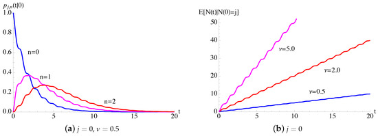
In Figure 3, for the $NHP$ process with $\nu \left(t\right)$ as in (25), the transition probabilities, given in (26), and the conditional mean, given in (27), are plotted as function of t for some choices of parameters. We note that the conditional mean increases linearly with a periodic modulation.

Figure 3. For the time-inhomogeneous Poisson ($NHP$) process, with $\nu \left(t\right)$ given in (25), the probabilities $p_{j,n}\left(t\right|0)$ (a) and the conditional mean (b) are plotted as function of t for $a=0.9$, $Q=1.0$.

3.2. Time-Inhomogeneous Linear Birth Process

We consider the time-inhomogeneous linear birth ($NHB$) process having state-space $\{j,j+1,\dots \}$, conditioned to start from $j\in \mathbb{N}$ at time $t_0$. We assume that the birth intensity function is ${\lambda }_n\left(t\right)=n\lambda \left(t\right)$ for $n=j,j+1,\dots$, with $\lambda \left(t\right)$ positive, bounded and continuous function for $t\ge t_0$. This process is also called “generalized inhomogeneous Yule–Furry process” (cf., for instance, Konno [34]). The NHB process can be used to modeling the growth of a population of unicellular organism, such as bacteria, taking into account that whenever two new organisms born, the reproducing individual ceases to exist. The NHB process can also describe population models in which the parent organism coexists with the newly generated individual. In both the cases, the population size increases exactly by one unit as a result of a single reproduction (cf., for instance, Kendall [35], Van Den Broek and Heesterbeek [36]).

In the general $NHBDI$ process, we set $\nu \left(t\right)=\mu \left(t\right)=0$ and ${\lambda }_n\left(t\right)=n\lambda \left(t\right)$ for $n=j,j+1,\dots$, so that from (4) and (6) one has $M\left(t\right|t_0)=0$ and $A\left(t\right|t_0)=1-e^{-\Lambda \left(t\right|t_0)}$. Therefore, from (5), we obtain the probability generating function for the $NHB$ process:

$$G_j(z,t)={\left\{\frac{z{e}^{-\Lambda \left(t\right|t_0)}}{1-z\left[1-e^{-\Lambda \left(t\right|t_0)}\right]}\right\}}^j,j\in \mathbb{N},t\ge t_0.$$

Moreover, recalling (13) and (14), we have: $d_r=0$ for $r\in \mathbb{N}$, $B_0=1$ and $B_n(d_1,d_2,\dots ,d_n)=0$ for $n\in \mathbb{N}$. For the $NHB$ process, from (11) one has $\alpha \left(t\right|t_0)=0$, $\beta \left(t\right|t_0)=1-e^{-\Lambda \left(t\right|t_0)}$ for $t\ge t_0$, so that, by choosing $k=0$ and $r=j$ in (17), for $j\in \mathbb{N}$ and $t\ge t_0$ it follows:

$$p_{j,n}\left(t\right|t_0)=\left(\genfrac{}{}{0pt}{}{n-1}{j-1}\right){\left[1-e^{-\Lambda \left(t\right|t_0)}\right]}^{n-j}{e}^{-j\Lambda \left(t\right|t_0)},n=j,j+1,\dots ,$$

(28)

that is a shifted negative binomial distribution with success probability $e^{-\Lambda \left(t\right|t_0)}$. Finally, making use of (7), the conditional mean and the conditional variance for the $NHB$ process $N\left(t\right)$ are:

$$\mathrm{E}\left[N\left(t\right)\right|N\left(t_0\right)=j]=j{e}^{\Lambda \left(t\right|t_0)},\mathrm{Var}\left[N\left(t\right)\right|N\left(t_0\right)=j]=j{e}^{\Lambda \left(t\right|t_0)}\left[e^{\Lambda \left(t\right|t_0)}-1\right],j\in \mathbb{N},t\ge t_0.$$

We note that the conditional mean increases with t and tends to infinite when ${lim}_{t\to +\infty }\Lambda \left(t\right|t_0)=+\infty$.

3.3. Time-Inhomogeneous Linear Death Process

We consider the time-inhomogeneous linear death ($NHD$) process having state-space $\{0,1,\dots ,j\}$, conditioned to start from $j\in \mathbb{N}$ at time $t_0$. We assume that the death intensity function is ${\mu }_n\left(t\right)=n\mu \left(t\right)$ for $n=0,1,\dots ,j$, with $\mu \left(t\right)$ positive, bounded and continuous function for $t\ge t_0$. For the $NHD$ process, the population size decreases over time (cf., for instance, Ricciardi [6], Van Den Broek and Heesterbeek [36]).

In the general $NHBDI$ process, we set $\lambda \left(t\right)=\nu \left(t\right)=0$ and ${\mu }_n\left(t\right)=n\mu \left(t\right)$ for $n=0,1,\dots j$, so that from (4) and (6) one has $\Lambda \left(t\right|t_0)=0$ and $A\left(t\right|t_0)=0$. Then, from (5), we obtain the probability generating function for the $NHD$ process:

$$G_j(z,t)={\left[1+(z-1)e^{-M\left(t\right|t_0)}\right]}^j,j\in \mathbb{N},t\ge t_0.$$

Furthermore, making use of (13) and (14), we have: $d_r=0$ for $r\in \mathbb{N}$, $B_0=1$ and $B_n(d_1,d_2,\dots ,d_n)=0$ for $n\in \mathbb{N}$. For the $NHD$ process, from (11) one has $\alpha \left(t\right|t_0)=1-e^{-M\left(t\right|t_0)}$, $\beta \left(t\right|t_0)=0$ for $t\ge t_0$, so that, by choosing $k=0$ and $r=n$ in (17), for $j\in \mathbb{N}$ and $t\ge t_0$ one obtains:

$$p_{j,n}\left(t\right|t_0)=\left(\genfrac{}{}{0pt}{}{j}{n}\right){\left[1-e^{-M\left(t\right|t_0)}\right]}^{j-n}{e}^{-nM\left(t\right|t_0)},n=0,1,\dots j,$$

(29)

that is a binomial distribution with success probability $e^{-M\left(t\right|t_0)}$.

Then, when ${lim}_{t\to +\infty }M\left(t\right|t_0)=+\infty$, one has ${lim}_{t\to +\infty }{p}_{j,0}\left(t\right|t_0)=1$, implying that the asymptotic extinction of the population is a sure event. Making use of (7), the conditional mean and the conditional variance for the $NHD$ process $N\left(t\right)$ are:

$$\mathrm{E}\left[N\left(t\right)\right|N\left(t_0\right)=j]=j{e}^{-M\left(t\right|t_0)},\mathrm{Var}\left[N\left(t\right)\right|N\left(t_0\right)=j]=j{e}^{-M\left(t\right|t_0)}\left[1-e^{-M\left(t\right|t_0)}\right],j\in \mathbb{N},t\ge t_0.$$

Finally, we note that the conditional mean decreases with t and approaches to zero when ${lim}_{t\to +\infty }M\left(t\right|t_0)=+\infty$ according to the fact that the population is doomed to extinction.

3.4. Time-Inhomogeneous Linear Birth–Death Process

The linear birth–death process ($NHBD$) process is obtained by combining the assumptions underlying the $NHB$ and the $NHD$ processes (cf., for instance, Bailey [1], Kendall [35] and Tavaré [37]). We now consider the $NHBD$ process having space-state ${\mathbb{N}}_0$, conditioned to start from $j\in \mathbb{N}$ at time $t_0$. We assume that the birth and death intensity functions are ${\lambda }_n\left(t\right)=n\lambda \left(t\right)$ and ${\mu }_n\left(t\right)=n\mu \left(t\right)$, respectively, with $\lambda \left(t\right)$ and $\mu \left(t\right)$ positive, bounded and continuous functions for $t\ge t_0$.

In the general $NHBDI$ process, we set $\nu \left(t\right)=0$, ${\lambda }_n\left(t\right)=n\lambda \left(t\right)$ and ${\mu }_n\left(t\right)=n\mu \left(t\right)$ for $n\in \mathbb{N}$. Hence, from (5) we derive the probability generating function for the $NHBD$ process:

$$G_j(z,t)={\left[\frac{1+(z-1)e^{\Lambda \left(t\right|t_0)-M\left(t\right|t_0)}[1-A\left(t\right|t_0)]}{1-(z-1)e^{\Lambda \left(t\right|t_0)-M\left(t\right|t_0)}A\left(t\right|t_0)]}\right]}^j,j\in \mathbb{N},t\ge t_0,$$

where $\Lambda \left(t\right|t_0)$, $M\left(t\right|t_0)$ and $A\left(t\right|t_0)$ are defined in (4) and (6), respectively. Recalling (13) and (14), we have: $d_r=0$ for $r\in \mathbb{N}$, $B_0=1$ and $B_n(d_1,d_2,\dots ,d_n)=0$ for $n\in \mathbb{N}$. Furthermore, by choosing $k=0$ in (17), for $j\in \mathbb{N}$ and $t\ge t_0$ one obtains:

$$p_{j,n}\left(t\right|t_0)=\sum _{r=0}^{min(n,j)}\left(\genfrac{}{}{0pt}{}{j}{r}\right)\left(\genfrac{}{}{0pt}{}{j+n-r-1}{j-1}\right){\left[\alpha \left(t\right|t_0)\right]}^{j-r}{\left[\beta \left(t\right|t_0)\right]}^{n-r}{[1-\alpha \left(t\right|t_0)-\beta \left(t\right|t_0)]}^r,n\in {\mathbb{N}}_0,$$

(30)

where $\alpha \left(t\right|t_0)$ and $\beta \left(t\right|t_0)$ are defined in (11). For the $NHBD$ process, the use of (7) for $j\in \mathbb{N}$ and $t\ge t_0$ leads to:

$$\begin{array}{c}\mathrm{E}\left[N\left(t\right)\right|N\left(t_0\right)=j]=j{e}^{\Lambda \left(t\right|t_0)-M\left(t\right|t_0)},\\ \mathrm{Var}\left[N\left(t\right)\right|N\left(t_0\right)=j]=j{e}^{\Lambda \left(t\right|t_0)-M\left(t\right|t_0)}\left\{1-e^{\Lambda \left(t\right|t_0)-M\left(t\right|t_0)}+2A\left(t\right|t_0)e^{\Lambda \left(t\right|t_0)-M\left(t\right|t_0)}\right\}.\end{array}$$

(31)

Moreover, by setting $n=0$ in (30), for $j\in \mathbb{N}$ one has:

$$p_{j,0}\left(t\right|t_0)=[\alpha {\left(t\right|t_0]}^j={\left[1-\frac{1}{1+{\int }_{t_0}^t\mu \left(\tau \right)e^{M\left(\tau \right|t_0)-\Lambda \left(\tau \right|t_0)}d\tau }\right]}^j,$$

(32)

so that for the $NHBD$ process the probability of ultimate extinction tends to unity as $t\to +\infty$ if and only if

$$\underset{t\to +\infty }{lim}{\int }_{t_0}^t\mu \left(\tau \right)e^{M\left(\tau \right|t_0)-\Lambda \left(\tau \right|t_0)}d\tau =+\infty .$$

Time-Homogeneous Linear Birth–Death Process

A special case is the time-homogeneous linear birth–death ($HBD$) process, characterized by birth and death rates ${\lambda }_n\left(t\right)=n\lambda$ and ${\mu }_n\left(t\right)=n\mu$ for $n\in {\mathbb{N}}_0$, with $\lambda$ and $\mu$ positive real numbers (cf., for instance, Bailey [1], Ricciardi [6] and Crawford and Suchard [9]). For the $HBD$ process, by assuming that $\nu \to 0$ in (20) and in (21), we obtain the transition probabilities. For $\lambda \ne \mu$ and $j\in \mathbb{N}$ one has:

$$p_{j,n}\left(t\right|t_0)=\sum _{r=0}^{min(j,n)}\left(\genfrac{}{}{0pt}{}{j}{r}\right)\left(\genfrac{}{}{0pt}{}{j+n-r-1}{j-1}\right){\left[\mu \varrho \left(t\right|t_0)\right]}^{j-r}{\left[\lambda \varrho \left(t\right|t_0)\right]}^{n-r}{[1-(\lambda +\mu )\varrho \left(t\right|t_0)]}^r,n\in {\mathbb{N}}_0,$$

(33)

with $\varrho \left(t\right|t_0)$ defined in (19), whereas, for $\lambda =\mu$ and $j\in \mathbb{N}$ one obtains:

$$p_{j,n}\left(t\right|t_0)=\sum _{r=0}^{min(j,n)}\left(\genfrac{}{}{0pt}{}{j}{r}\right)\left(\genfrac{}{}{0pt}{}{j+n-r-1}{j-1}\right){\left[\frac{1-\lambda (t-t_0)}{\lambda (t-t_0)}\right]}^r{\left[\frac{\lambda (t-t_0)}{1+\lambda (t-t_0)}\right]}^{j+n-r},n\in {\mathbb{N}}_0.$$

(34)

Moreover, from (33) and (34), for $j\in \mathbb{N}$ and $t\ge t_0$ it follows:

$$\underset{t\to +\infty }{lim}{p}_{j,0}\left(t\right|t_0)=\left\{\begin{array}{cc}1,\hfill & \lambda \le \mu ,\hfill \\ {\displaystyle {\left(\frac{\mu }{\lambda }\right)}^j}\hfill & \lambda >\mu .\hfill \end{array}\right.$$

Hence, for the $HBD$ process the probability of ultimate extinction tends to unity as $t\to +\infty$ if and only if $\lambda \le \mu$. Furthermore, for $\nu \to 0$ in (22), one derives the conditional mean and conditional variance for the $HBD$ process:

$$\begin{array}{c}\mathrm{E}\left[N\left(t\right)\right|N\left(t_0\right)=j]=\left\{\begin{array}{cc}{\displaystyle j,}\hfill & \lambda =\mu ,\hfill \\ {\displaystyle j{e}^{(\lambda -\mu )(t-t_0)},}\hfill & \lambda \ne \mu ,\hfill \end{array}\right.\hfill \\ \hfill \\ \mathrm{Var}\left[N\left(t\right)\right|N\left(t_0\right)=j]=\left\{\begin{array}{cc}2j\lambda (t-t_0),\hfill & \lambda =\mu ,\hfill \\ {\displaystyle \frac{j(\lambda +\mu )}{\lambda -\mu }{e}^{(\lambda -\mu )(t-t_0)}\left[e^{(\lambda -\mu )(t-t_0)}-1\right],}\hfill & \lambda \ne \mu .\hfill \end{array}\right.\hfill \end{array}$$

(35)

Then, for the $HBD$ process the mean population size exponentially increases for $\lambda >\mu$, exponentially decreases if $\lambda <\mu$ and remains constant if $\lambda =\mu$.

In Figure 4, the conditional mean and the conditional variance (35) of the $HBD$ process are plotted as function of t for some choices of $\lambda$ and $\mu$.

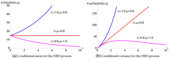
Figure 4. For the time-homogeneous linear birth–death ($HBD$) process, the conditional mean and the conditional variance (35) are plotted as function of t, with $j=15$, for some choices of $\lambda$ and $\mu$.

3.5. Time-Inhomogeneous Linear Death Process with Immigration

We consider the time-inhomogeneous linear death with immigration ($NHDI$) process having state-space ${\mathbb{N}}_0$, conditioned to start from $j\in {\mathbb{N}}_0$ at time $t_0$. We assume that the birth and death intensity functions are ${\lambda }_n\left(t\right)=\nu \left(t\right)$ and ${\mu }_n\left(t\right)=n\mu \left(t\right)$ for $n\in {\mathbb{N}}_0$, with $\nu \left(t\right)$ and $\mu \left(t\right)$ positive, bounded and continuous functions for $t\ge t_0$ (cf., for instance, Ohkubo [38]). The $NHDI$ process also describes the multi-server queuing systems $M\left(t\right)/M\left(t\right)/\infty$ in which the arrivals are governed by a time-inhomogeneous Poisson process with intensity function $\nu \left(t\right)$, there are infinitely many servers in parallel and the service times have an non-homogeneous exponential density with intensity function $\mu \left(t\right)$. In the $M\left(t\right)/M\left(t\right)/\infty$ queue, there are always sufficient servers such that every arriving job is served immediately (cf., for instance, Di Crescenzo et al. [8], Giorno et al. [23]).

In the general $NHBDI$ process, we set $\lambda \left(t\right)=0$, ${\lambda }_n\left(t\right)=\nu \left(t\right)$ and ${\mu }_n\left(t\right)=n\mu \left(t\right)$ for $n\in {\mathbb{N}}_0$. Hence, from (5) we derive the probability generating function for the $NHDI$ process:

$$G_j(z,t)=exp\left\{(z-1){\int }_{t_0}^t\nu \left(u\right)e^{-M\left(t\right|u)}du\right\}{\left[1+(z-1)e^{-M\left(t\right|t_0)}\right]}^j,j\in {\mathbb{N}}_0,t\ge t_0,$$

with $M\left(t\right|t_0)$ defined in (4). Recalling (13) and (14) we have $d_1={\int }_{t_0}^t\nu \left(u\right)e^{-M\left(t\right|u)}du$, $d_r=0$ for $r=2,3,\dots$ and

$$B_0=1,B_n(d_1,d_2,\dots ,d_n)={\left[{\int }_{t_0}^t\nu \left(u\right)e^{-M\left(t\right|u)}du\right]}^n,n\in \mathbb{N}.$$

For the $NHDI$ process, from (11) it results $\alpha \left(t\right|t_0)=1-e^{-M\left(t\right|t_0)}$ and $\beta \left(t\right|t_0)=0$ for $t\ge t_0$. Then, for the $NHDI$ process from (12) we obtain the time-inhomogeneous Poisson distribution:

$$p_{0,n}\left(t\right|t_0)=exp\left\{-{\int }_{t_0}^t\nu \left(u\right)e^{-M\left(t\right|u)}du\right\}\frac{1}{n!}{\left[{\int }_{t_0}^t\nu \left(u\right)e^{-M\left(t\right|u)}du\right]}^n,n\in {\mathbb{N}}_0,t\ge t_0.$$

Furthermore, from (17) for $t\ge t_0$ we have:

$$\begin{array}{ccc}\hfill & \hfill & {\displaystyle p_{j,n}\left(t\right|t_0)=exp\left\{-{\int }_{t_0}^t\nu \left(u\right)e^{-M\left(t\right|u)}du\right\}\sum _{\ell =0}^{min(j,n)}\frac{1}{(n-\ell )!}\left(\genfrac{}{}{0pt}{}{j}{\ell }\right)e^{-\ell M\left(t\right|t_0)}}\hfill \\ \hfill & \hfill & \times {\left[1-e^{-M\left(t\right|t_0)}\right]}^{j-\ell }{\left[{\int }_{t_0}^t\nu \left(u\right)e^{-M\left(t\right|u)}du\right]}^{n-\ell }j\in \mathbb{N},n\in {\mathbb{N}}_0.\hfill \end{array}$$

(36)

For the $NHDI$ process, making use of (7), for $j\in {\mathbb{N}}_0$ and $t\ge t_0$ one obtains the conditional mean and the conditional variance:

$$\begin{array}{cc}\hfill & \mathrm{E}\left[N\left(t\right)\right|N\left(t_0\right)=j]=j{e}^{-M\left(t\right|t_0)}+{\int }_{t_0}^t\nu \left(u\right)e^{-M\left(t\right|u)}du,\hfill \\ \hfill & \mathrm{Var}\left[N\left(t\right)\right|N\left(t_0\right)=j]=j{e}^{-M\left(t\right|t_0)}\left[1-e^{-M\left(t\right|t_0)}\right]+{\int }_{t_0}^t\nu \left(u\right)e^{-M\left(t\right|u)}du.\hfill \end{array}$$

(37)

Time-Homogeneous Linear Death Process with Immigration

A special case is the time-homogeneous linear death-immigration ($HDI$) process, characterized by birth and death rates ${\lambda }_n\left(t\right)=\nu$ and ${\mu }_n\left(t\right)=n\mu$ for $n\in {\mathbb{N}}_0$, with $\nu$ and $\mu$ positive real numbers. The $HDI$ process can be used to describe the $M/M/\infty$ queuing system with infinitely many servers in parallel, exponential interarrival and service times with mean $1/\nu$ and $1/\mu$, respectively (cf., for instance, Medhi [5], Di Crescenzo et al. [8] and Giorno et al. [23]). For the $HDI$ process, by setting $\lambda =0$ in (20), for $t\ge t_0$ we obtain the transition probabilities:

$$\begin{array}{c}{p}_{0,n}\left(t\right|t_0)=exp\left\{-\frac{\nu }{\mu }\left[1-e^{-\mu (t-t_0)}\right]\right\}\frac{1}{n!}{\left\{\frac{\nu }{\mu }\left[1-e^{-\mu (t-t_0)}\right]\right\}}^n,n\in {\mathbb{N}}_0,\hfill \\ \hfill \\ p_{j,n}\left(t\right|t_0)=exp\left\{-\frac{\nu }{\mu }\left[1-e^{-\mu (t-t_0)}\right]\right\}\sum _{\ell =0}^{min(j,n)}\frac{1}{(n-\ell )!}\left(\genfrac{}{}{0pt}{}{j}{\ell }\right){\left(\frac{\nu }{\mu }\right)}^{n-\ell }{e}^{-\ell \mu h\left(t\right|t_0)}{\left[1-e^{-\mu (t-t_0)}\right]}^{j+n-2\ell },\hfill \\ j\in \mathbb{N},n\in {\mathbb{N}}_0\hfill \end{array}$$

(38)

and for $\lambda \to 0$ in (22), for $j\in {\mathbb{N}}_0$ and $t\ge t_0$ we obtain the conditional mean and the conditional variance of the $HDI$ process:

$$\begin{array}{c}\mathrm{E}\left[N\left(t\right)\right|N\left(t_0\right)=j]=j{e}^{-\mu (t-t_0)}+\frac{\nu }{\mu }\left[1-e^{-\mu (t-t_0)}\right],\hfill \\ \mathrm{Var}\left[N\left(t\right)\right|N\left(t_0\right)=j]=\left[j{e}^{-\mu (t-t_0)}+\frac{\nu }{\mu }\right]\left[1-e^{-\mu (t-t_0)}\right].\hfill \end{array}$$

Furthermore, from (38) it follows that the $HDI$ process always admits the Poisson steady-state distribution:

$$q_n=\underset{t\to +\infty }{lim}{p}_{0,n}\left(t\right|t_0)=\frac{1}{n!}{\left(\frac{\nu }{\mu }\right)}^n{e}^{-\nu /\mu },n\in \mathbb{N},$$

(39)

so that the asymptotic mean and variance are $\mathrm{E}\left(N\right)=\mathrm{Var}\left(N\right)=\nu /\mu$.

Example 3.

We consider the $NHDI$ process $N\left(t\right)$, with $t_0=0$, characterized by ${\lambda }_n\left(t\right)=\nu \left(t\right)$ and ${\mu }_n\left(t\right)=\mu n$, with $\mu >0$, subject to periodic immigration phenomena that occur with intensity function (25). This process can describe a queuing system $M\left(t\right)/M/\infty$, in which the customers arrive according to a time-inhomogeneous Poisson process with the periodic intensity function (25).

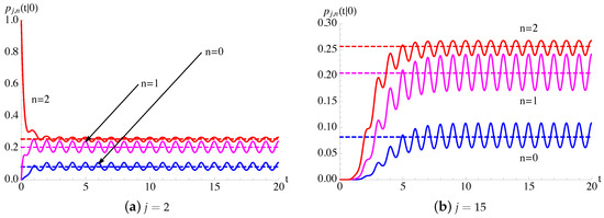
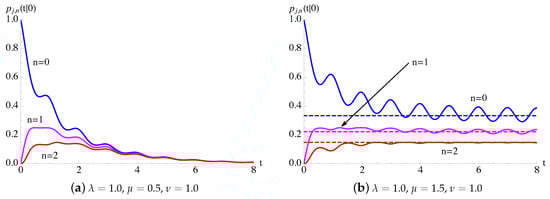
In Figure 5, the transition probabilities $p_{j,n}\left(t\right|0)$, given in (36), for the $NHDI$ process with constant death rate and periodic immigration intensity function (25) are plotted as function of t for $j=2,15$ and $n=0,1,2$ for some fixed choices of parameters. We note that, for large times, the transition probabilities $p_{j,n}\left(t\right|0)$ oscillate around the probabilities $q_n$, given in (39), related to the $HDI$ process.

Figure 5. For the $NHDI$ process, having ${\lambda }_n\left(t\right)=\nu \left(t\right)$ and ${\mu }_n\left(t\right)=\mu n$, with $\nu \left(t\right)$ given in (25), the probabilities $p_{j,n}\left(t\right|0)$ are plotted as function of t for $\mu =0.8$, $\nu =2.0$, $a=0.9$, $Q=1.0$ with $n=0,1,2$. The dashed lines indicate the probabilities $q_0$, $q_1$, $q_2$, given in (39).

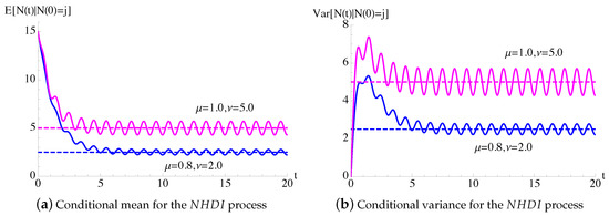
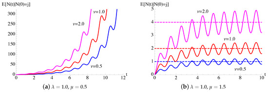
In Figure 6, the conditional mean and the conditional variance, given in (37), of the $NHDI$ process of Figure 5 are plotted as function of t for $j=15$, $a=0.9$, $Q=1.0$ and some choices of μ and ν. The dashed lines indicate $\mathrm{E}\left(N\right)=\mathrm{Var}\left(N\right)=\nu /\mu$, related to $HDI$ process. In the $M\left(t\right)/M/\infty$ queue this means that, for large times, the number of the customers exhibits a periodic behavior, which strongly depends on the periodicity of the arrivals in the system.

Figure 6. For the $NHDI$ process of Figure 5, the conditional mean and the conditional variance (37) are plotted as function of t for $j=15$, $a=0.9$, $Q=1.0$ and for some choices of μ and ν. The dashed lines indicate the asymptotic mean and the asymptotic variance of the $HBDI$ process, given in (24).

3.6. Time Inhomogeneous Linear Birth Process with Immigration

We consider the time-inhomogeneous linear birth with immigration ($NHBI$) process having state-space $\{j,j+1,\dots \}$, conditioned to start to $j\in {\mathbb{N}}_0$ at time $t_0$. We assume that the birth intensity function is ${\lambda }_n\left(t\right)=\lambda \left(t\right)n+\nu \left(t\right)$ for $n=j,j+1,\dots$, with $\lambda \left(t\right)$ and $\nu \left(t\right)$ positive, bounded and continuous functions for $t\ge t_0$. In the $NHBI$ process a new individual can be regarded as arising from two sources, one involving the time-inhomogeneous Poisson process with intensity function $\nu \left(t\right)$, the other being a linear time-inhomogeneous birth process with intensity function $\lambda \left(t\right)$ for individual.

In the general $NHBDI$ process, we set $\mu \left(t\right)=0$ and ${\lambda }_n\left(t\right)=\lambda \left(t\right)n+\nu \left(t\right)$ for $n\in {\mathbb{N}}_0$, so that from (4) and (6) one has $M\left(t\right|t_0)=0$ and $A\left(t\right|t_0)=1-e^{-\Lambda \left(t\right|t_0)}$. Therefore, from (5), the probability generating function follows:

$$G_j(z,t)=exp\left\{(z-1){\int }_{t_0}^t\frac{\nu \left(u\right)}{1-z\left(1-e^{-\Lambda \left(t\right|u)}\right)}du\right\}{\left[\frac{z{e}^{-\Lambda \left(t\right|t_0)}}{1-z\left(1-e^{-\Lambda \left(t\right|t_0)}\right)}\right]}^j,j\in {\mathbb{N}}_0,t\ge t_0.$$

(40)

Furthermore, by virtue of (14), one has:

$$d_r=r!e^{-\Lambda \left(t\right|t_0)}{\int }_{t_0}^t\nu \left(u\right)e^{r\Lambda \left(u\right|t_0)}{\left[e^{-\Lambda \left(u\right|t_0)})-e^{-\Lambda \left(t\right|t_0)})\right]}^{r-1}du,r\in \mathbb{N},$$

(41)

and the complete Bell polynomials can be derived via the recurrence Equation (13). For the $NHBI$ process, from (11) we obtain $\alpha \left(t\right|t_0)=0$ and $\beta \left(t\right|t_0)=1-e^{-\Lambda \left(t\right|t_0)}$ for $t\ge t_0$. Then, for the $NHBI$ process from (12) we obtain

$$p_{0,n}\left(t\right|t_0)=exp\left\{-{\int }_{t_0}^t\nu \left(u\right)du\right\}\frac{B_n(d_1,d_2,\dots ,d_n)}{n!},n\in {\mathbb{N}}_0,t\ge t_0.$$

(42)

Furthermore, by setting $k=0,1,n-j$ and $r=j$ in (17), for $t\ge t_0$ we have:

$$\begin{array}{c}{p}_{j,n}\left(t\right|t_0)=exp\left\{-{\int }_{t_0}^t\nu \left(u\right)du\right\}{e}^{-j\Lambda \left(t\right|t_0)}\sum _{k=0}^{n-j}\frac{B_k(d_1,d_2,\dots ,d_k)}{k!}\left(\genfrac{}{}{0pt}{}{n-k-1}{j-1}\right){\left[1-e^{-\Lambda \left(t\right|t_0)}\right]}^{n-k-j},\hfill \\ n=j,j+1,\dots ;j\in \mathbb{N}.\hfill \end{array}$$

(43)

For the $NHBI$ process, making use of (7), for $j\in {\mathbb{N}}_0$ and $t\ge t_0$ one obtains the conditional mean and the conditional variance:

$$\begin{array}{cc}\hfill & \mathrm{E}\left[N\left(t\right)\right|N\left(t_0\right)=j]=j{e}^{\Lambda \left(t\right|t_0)}+{\int }_{t_0}^t\nu \left(u\right)e^{\Lambda \left(t\right|u)}du,\hfill \\ \hfill & \mathrm{Var}\left[N\left(t\right)\right|N\left(t_0\right)=j]=j{e}^{\Lambda \left(t\right|t_0)}\left[e^{\Lambda \left(t\right|t_0)}-1\right]+{\int }_{t_0}^t\nu \left(u\right)e^{\Lambda \left(t\right|u)}du+2{\int }_{t_0}^t\nu \left(u\right)e^{2\Lambda \left(t\right|u)}du.\hfill \end{array}$$

(44)

Time-Homogeneous Linear Birth Immigration Process

A special case is the time-homogeneous linear birth immigration ($HBI$) process, characterized by birth and death rates ${\lambda }_n\left(t\right)=n\lambda +\nu$ for $n=j,j+1,\dots$ and $j\in {\mathbb{N}}_0$, with $\lambda$ and $\nu$ positive real numbers (cf., for instance, Tavaré [12]). For the $HBI$ process, by setting $\mu =0$ in (20), for $t\ge t_0$ we obtain the transition probabilities:

$$p_{j,n}\left(t\right|t_0)=\frac{1}{(n-j)!}{\left(j+\frac{\nu }{\lambda }\right)}_{n-j}{e}^{-(\lambda j+\nu )(t-t_0)}{\left[1-e^{-\lambda (t-t_0)}\right]}^{n-j},n=j,j+1,\dots ;j\in {\mathbb{N}}_0.$$

(45)

Furthermore, for $\mu \to 0$ in (22), for $j\in {\mathbb{N}}_0$ and $t\ge t_0$ we have the conditional mean and the conditional variance of the $HBI$ process:

$$\begin{array}{c}\mathrm{E}\left[N\left(t\right)\right|N\left(t_0\right)=j]=j{e}^{\lambda (t-t_0)}+\frac{\nu }{\lambda }\left[e^{\lambda (t-t_0)}-1\right],\hfill \\ \hfill \\ \mathrm{Var}\left[N\left(t\right)\right|N\left(t_0\right)=j]=\left(j+\frac{\nu }{\lambda }\right)e^{\lambda (t-t_0)}\left[e^{\lambda (t-t_0)}-1\right].\hfill \end{array}$$

(46)

Example 4.

We consider the $NHBI$ process $N\left(t\right)$, with $t_0=0$, characterized by ${\lambda }_n\left(t\right)=\lambda n+\nu \left(t\right)$, with $\lambda >0$, subject to periodic immigration phenomena that occur with intensity function (25).

In Figure 7, the transition probabilities $p_{j,n}\left(t\right|0)$, given in (42) and in (43), for the $NHBI$ process with constant birth rate and periodic immigration intensity function (25) are plotted as function of t for $j=0$ and $n=0,1,2$ for some choices of parameters.

Figure 7. For the $NHBI$ process, having ${\lambda }_n\left(t\right)=\lambda n+\nu \left(t\right)$, with $\nu \left(t\right)$ given in (25), the probabilities $p_{j,n}\left(t\right|0)$ are plotted for $a=0.9$, $Q=1.0$ with $n=0,1,2$.

In Figure 8, the conditional mean and the conditional variance, given in (44), of the $NHBI$ process of Figure 7 are plotted as function of t for $j=0$, $a=0.9$, $Q=1.0$ and some choices of λ and ν. We note that the shapes of the conditional mean and of the conditional variance are little influenced by the periodicity of $\nu \left(t\right)$.

Figure 8. For the $NHBI$ process of Figure 7, the conditional mean and the conditional variance (44) are plotted as function of t for $j=0$, $a=0.9$, $Q=1.0$ and for some choices of λ and ν.

3.7. Generalized Polya Process

We consider the generalized Polya ($GPy$) process $\{N\left(t\right),t\ge t_0\}$, obtained by setting $\nu \left(t\right)=\nu \lambda \left(t\right)$ in the $NHBI$ process. Then, in the $GPy$ process we assume that the birth intensity function is ${\lambda }_n\left(t\right)=\lambda \left(t\right)(n+\nu )$ for $n=j,j+1,\dots$, with $\nu$ positive real number and $\lambda \left(t\right)$ positive, bounded and continuous function for $t\ge t_0$ (cf., for instance, Konno [34]). We note that the $GPy$ process is a generalization of the Polya process, characterized by intensity function:

$${\lambda }_n\left(t\right)=\frac{\alpha (1+\beta n)}{1+\alpha \beta t},n=j,j+1,\dots ;j\in {\mathbb{N}}_0,t\ge t_0.$$

(47)

Indeed, the Polya process is obtained by setting $\lambda \left(t\right)=\alpha \beta /(1+\alpha \beta t)$ and $\nu =1/\beta$ in the $GPy$ process. In the literature, the Polya process has been considered in the treatment of electron-photon cascade theory, with decay factor ${(1+\alpha \beta t)}^{-1}$ (cf., for instance, Bailey [1] and Ricciardi [6]).

For the $GPy$ process, recalling that $\nu \left(t\right)=\nu \lambda \left(t\right)$, from (40) one has:

$$G_j(z,t)=\frac{z^j{e}^{-(j+\nu )\Lambda \left(t\right|t_0)}}{{\{1-z(1-e^{-\Lambda \left(t\right|t_0)})\}}^{j+\nu }},j\in {\mathbb{N}}_0,t\ge t_0.$$

(48)

Moreover, from (41) we have $d_r=\nu (r-1)!{\left[1-e^{-\Lambda \left(t\right|t_0)}\right]}^r$ for $r\in \mathbb{N}$, so that from (13) we have $B_0=1$ and

$$B_{n+1}(d_1,d_2,\dots ,d_{n+1})=\nu n!\sum _{i=0}^n\frac{1}{(n-i)!}{B}_{n-i}(d_1,d_2,\dots ,d_{n-i}){\left[1-e^{-\Lambda \left(t\right|t_0)}\right]}^{i+1},n\in {\mathbb{N}}_0.$$

(49)

The solution of the recurrence equation (49) is:

$$B_n(d_1,d_2,\dots ,d_n)={\left(\nu \right)}_n{\left[1-e^{-\Lambda \left(t\right|t_0)}\right]}^n,n\in {\mathbb{N}}_0,$$

(50)

obtained by using the following identities:

$${\left(z\right)}_k=\frac{\Gamma (z+k)}{\Gamma \left(z\right)},\sum _{k=0}^n\frac{{\left(a\right)}_k}{k!}=\frac{\Gamma (a+n+1)}{\Gamma (a+1)n!},n\in {\mathbb{N}}_0,$$

with $\Gamma \left(x\right)$ denoting the Euler’s gamma function. By virtue of (50), from (42) and (43) for $t\ge t_0$ one obtains the transition probabilities of the $GPy$ process:

$$\begin{array}{c}{p}_{0,n}\left(t\right|t_0)=\frac{{\left(\nu \right)}_n}{n!}{e}^{-\nu \Lambda \left(t\right|t_0)}{\left[1-e^{-\Lambda \left(t\right|t_0)}\right]}^n,n\in {\mathbb{N}}_0,\hfill \\ \hfill \\ p_{j,n}\left(t\right|t_0)=e^{-(\nu +j)\Lambda \left(t\right|t_0)}{\left[1-e^{-\Lambda \left(t\right|t_0)}\right]}^{n-j}\sum _{k=0}^{n-j}\frac{{\left(\nu \right)}_k}{k!}\left(\genfrac{}{}{0pt}{}{n-k-1}{j-1}\right)\hfill \\ =\frac{\Gamma (\nu +n)}{(n-j)!\Gamma (\nu +j)}{e}^{-(\nu +j)\Lambda \left(t\right|t_0)}{\left[1-e^{-\Lambda \left(t\right|t_0)}\right]}^{n-j},n=j,j+1,\dots ;j\in \mathbb{N},\hfill \end{array}$$

(51)

where the last identity follows by noting that

$$\sum _{k=0}^i\frac{{\left(\nu \right)}_k}{k!}\left(\genfrac{}{}{0pt}{}{j+i-k-1}{j-1}\right)=\frac{{(\nu +j)}_i}{i!},i\in {\mathbb{N}}_0·$$

(52)

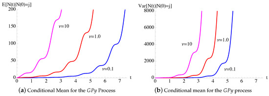
Finally, from (44), for $j\in {\mathbb{N}}_0$ and $t\ge t_0$ the conditional mean and the conditional variance of the $GPy$ process can be derived:

$$\mathrm{E}\left[N\left(t\right)\right|N\left(t_0\right)=j]=j{e}^{\Lambda \left(t\right|t_0)}+\nu \left[e^{\Lambda \left(t\right|t_0)}-1\right],\mathrm{Var}\left[N\left(t\right)\right|N\left(t_0\right)=j]=(j+\nu )e^{\Lambda \left(t\right|t_0)}\left[e^{\Lambda \left(t\right|t_0)}-1\right].$$

(53)

Example 5.

We consider the $GPy$ process $N\left(t\right)$, with $t_0=0$, characterized by ${\lambda }_n\left(t\right)=\lambda \left(t\right)(n+\nu )$, with $\nu >0$ and

$$\lambda \left(t\right)=\lambda \left[1+asin\left(\frac{2\pi t}{Q}\right)\right],t\ge 0,$$

(54)

with $\lambda >0$ and $0\le a<1$.

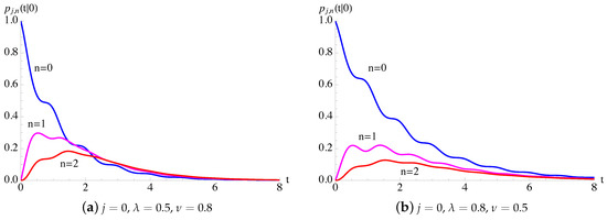
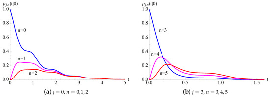
In Figure 9, the transition probabilities $p_{j,n}\left(t\right|0)$, given in (51), of the $GPy$ process with $\lambda \left(t\right)$ given in (54) are plotted as function of t for $j=0$ (on the left) and $j=3$ (on the right) for $a=0.9$, $Q=1.0$ and $\lambda =\nu =1.0$.

Figure 9. For the generalized Polya ($GPy$) process, having ${\lambda }_n\left(t\right)=\lambda \left(t\right)(n+\nu )$, with $\lambda \left(t\right)$ given in (54), the probabilities $p_{j,n}\left(t\right|0)$ are plotted as function of t for $a=0.9$, $Q=1.0$ and $\lambda =\nu =1.0$.

In Figure 10, the conditional mean and the conditional variance, given in (53), of the $GPy$ process of Figure 9 are plotted as function of t for $j=0$, $\lambda =1.0$, $a=0.9$, $Q=1.0$ and some choices of ν.

Figure 10. For the $GPy$ process of Figure 9, the conditional mean and the conditional variance (53) are plotted as function of t for $j=0$, $\lambda =1.0$, $a=0.9$, $Q=1.0$ and for some choices of ν.

3.8. Generalized Polya-Death Process

We consider the generalized Polya-death ($GPyD$) process $\{N\left(t\right),t\ge t_0\}$, obtained by setting $\nu \left(t\right)=\nu \lambda \left(t\right)$ in the $NHBDI$ process. Then, in the $GPyD$ process we assume that the birth and death intensity functions are ${\lambda }_n\left(t\right)=\lambda \left(t\right)(n+\nu )$ for $n\in {\mathbb{N}}_0$ and ${\mu }_n\left(t\right)=n\mu \left(t\right)$ for $n\in \mathbb{N}$, with $\nu$ positive real number and $\lambda \left(t\right)$, $\mu \left(t\right)$ bounded and continuous functions for $t\ge t_0$ (cf., for instance, Ohkubo [39]). A special case of $GPyD$ process has been considered in Giorno et al. [23] and Di Crescenzo and Nobile [40] to describe a time-inhomogeneous adaptive queuing system, by assuming that ${\lambda }_n\left(t\right)=(\lambda n+\alpha )k\left(t\right)$ for $n\in {\mathbb{N}}_0$ and ${\mu }_n\left(t\right)=n\mu k\left(t\right)$ for $n\in \mathbb{N}$. Moreover, a time-homogeneous $GPyD$ process, characterized by ${\lambda }_n\left(t\right)=\lambda (n+\alpha )$ and ${\mu }_n\left(t\right)=n\mu$, has been used to describe an adaptive queuing system, known as “Model D” with panic-buying and compensatory reaction of service (cf., for instance, Conolly [2], Lenin et al. [11] and Giorno and Nobile [18]).

Recalling that $\nu \left(t\right)=\nu \lambda \left(t\right)$, from (5) one has:

$$\begin{array}{ccc}\hfill & \hfill & G_j(z,t)=exp\left\{\nu (z-1){\int }_{t_0}^t\frac{\lambda \left(u\right)e^{\Lambda \left(t\right|u)-M(t\left|u\right)}}{1-(z-1)e^{\Lambda \left(t\right|t_0)-M\left(t\right|t_0)}[A\left(t\right|t_0)-A\left(u\right|t_0)]}du\right\}\hfill \\ \hfill & \hfill & \times {\left[\frac{1+(z-1)e^{\Lambda \left(t\right|t_0)-M\left(t\right|t_0)}[1-A\left(t\right|t_0)]}{1-(z-1)e^{\Lambda \left(t\right|t_0)-M\left(t\right|t_0)}A\left(t\right|t_0)}\right]}^{j}j\in {\mathbb{N}}_0,t\ge t_0,\hfill \end{array}$$

(55)

with $A\left(t\right|t_0)$ given in (6). Since

$$\frac{d}{du}ln\left\{1-(z-1)e^{\Lambda \left(t\right|t_0)-M\left(t\right|t_0)}[A\left(t\right|t_0)-A\left(u\right|t_0)]\right\}=\frac{(z-1)\lambda \left(u\right)e^{\Lambda \left(t\right|t_0)-M\left(t\right|t_0)}}{1-(z-1)e^{\Lambda \left(t\right|t_0)-M\left(t\right|t_0)}[A\left(t\right|t_0)-A\left(u\right|t_0)]},$$

from (55) one obtains the probability generating function of the $GPyD$ process:

$$G_j(z,t)=\frac{{\left\{1+(z-1)e^{\Lambda \left(t\right|t_0)-M\left(t\right|t_0)}[1-A\left(t\right|t_0)]\right\}}^j}{{\left\{1-(z-1)e^{\Lambda \left(t\right|t_0)-M\left(t\right|t_0)}A\left(t\right|t_0)\right\}}^{j+\nu }},j\in {\mathbb{N}}_0,t\ge t_0.$$

(56)

From (14) it follows:

$$\begin{array}{ccc}\hfill & \hfill & d_r=-\nu (r-1)!e^{r[\Lambda \left(t\right|t_0)-M\left(t\right|t_0)]}{\int }_{t_0}^t\frac{d}{du}{\left[\frac{A\left(t\right|t_0)-A\left(u\right|t_0)}{1+e^{\Lambda \left(t\right|t_0)-M\left(t\right|t_0)}[A\left(t\right|t_0)-A\left(u\right|t_0)]}\right]}^{r}du\hfill \\ \hfill & \hfill & =\nu (r-1)!{\left[\frac{A\left(t\right|t_0)e^{\Lambda \left(t\right|t_0)-M\left(t\right|t_0)}}{1+A\left(t\right|t_0)e^{\Lambda \left(t\right|t_0)-M\left(t\right|t_0)}}\right]}^r,r\in \mathbb{N}.\hfill \end{array}$$

(57)

Therefore, from (13) we have $B_0=1$ and

$$B_n(d_1,d_2,\dots ,d_n)={\left(\nu \right)}_n{\left[\frac{A\left(t\right|t_0)e^{\Lambda \left(t\right|t_0)-M\left(t\right|t_0)}}{1+A\left(t\right|t_0)e^{\Lambda \left(t\right|t_0)-M\left(t\right|t_0)}}\right]}^n={\left(\nu \right)}_n{\left[\beta \left(t\right|t_0)\right]}^n,n\in {\mathbb{N}}_0,$$

(58)

with $\beta \left(t\right|t_0)$ defined in (11).

Proposition 4.

For $t\ge t_0$, the transition probabilities of the $GPyD$ process are:

$$\begin{array}{c}{p}_{0,n}\left(t\right|t_0)=\frac{1}{{[1+e^{\Lambda \left(t\right|t_0)-M\left(t\right|t_0)}A\left(t\right|t_0)]}^{\nu }}\frac{{\left(\nu \right)}_n{\left[\beta \left(t\right|t_0)\right]}^n}{n!},n\in {\mathbb{N}}_0,\hfill \end{array}$$

(59)

$$\begin{array}{c}{p}_{j,n}\left(t\right|t_0)=\frac{1}{{[1+e^{\Lambda \left(t\right|t_0)-M\left(t\right|t_0)}A\left(t\right|t_0)]}^{\nu }}\sum _{r=0}^{min(j,n)}\left(\genfrac{}{}{0pt}{}{j}{r}\right)\frac{\Gamma (\nu +j+n-r)}{(n-r)!\Gamma (\nu +j)}\hfill \\ \times {\left[\alpha \left(t\right|t_0)\right]}^{j-r}{\left[\beta \left(t\right|t_0)\right]}^{n-r}{[1-\alpha \left(t\right|t_0)-\beta \left(t\right|t_0)]}^r,j\in \mathbb{N},n\in {\mathbb{N}}_0.\hfill \end{array}$$

(60)

Proof. 

Thew proof is given in Appendix D. □

Finally, from (7) for $j\in {\mathbb{N}}_0$ we obtain the conditional mean and the conditional variance for the $GPyD$ process:

$$\begin{array}{c}\mathrm{E}\left[N\left(t\right)\right|N\left(t_0\right)=j]=j{e}^{\Lambda \left(t\right|t_0)-M\left(t\right|t_0)}+\nu {\int }_{t_0}^t\lambda \left(u\right)e^{\Lambda \left(t\right|u)-M(t\left|u\right)}du,\hfill \\ \mathrm{Var}\left[N\left(t\right)\right|N\left(t_0\right)=j]=j{e}^{\Lambda \left(t\right|t_0)-M\left(t\right|t_0)}\left\{1-e^{\Lambda \left(t\right|t_0)-M\left(t\right|t_0)}+2e^{\Lambda \left(t\right|t_0)-M\left(t\right|t_0)}A\left(t\right|t_0)\right\}\hfill \\ +\nu {\int }_{t_0}^t\lambda \left(u\right)e^{\Lambda \left(t\right|u)-M(t\left|u\right)}du+2\nu e^{\Lambda \left(t\right|t_0)-M\left(t\right|t_0)}{\int }_{t_0}^t\lambda \left(u\right)e^{\Lambda \left(t\right|u)-M(t\left|u\right)}\left[A\left(t\right|t_0)-A\left(u\right|t_0)\right]du.\hfill \end{array}$$

(61)

Example 6.

We consider the $GPyD$ process $N\left(t\right)$, with $t_0=0$, characterized by ${\lambda }_n\left(t\right)=\lambda \left(t\right)(n+\nu )$ and ${\mu }_n\left(t\right)=\mu n$, with $\mu >0$, $\nu >0$ and $\lambda \left(t\right)$ given in (54).

In Figure 11, the transition probabilities $p_{j,n}\left(t\right|0)$, given in (59) and (60), of the $GPyD$ process with $\lambda \left(t\right)$ given in (54), are plotted as function of t for $a=0.9$, $Q=1.0$, $\lambda =\nu =1.0$ and different choices of μ. The dashed lines in Figure 11b indicate the steady-state probabilities $q_0$, $q_1$, $q_2$ of the homogeneous Polya-death process having ${\lambda }_n\left(t\right)=\lambda (n+\nu )$ and ${\mu }_n\left(t\right)=\mu n$, obtained from (23) by changing ν with $\lambda \nu$.

Figure 11. For the generalized Polya-death ($GPyD$) process, having ${\lambda }_n\left(t\right)=\lambda \left(t\right)(n+\nu )$ and ${\mu }_n\left(t\right)=\mu n$, with $\lambda \left(t\right)$ given in (54), the probabilities $p_{j,n}\left(t\right|0)$ are plotted as function of t for $j=0$, $a=0.9$, $Q=1.0$ and $n=0,1,2$.

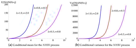
In Figure 12, the conditional mean, given in (61), of the $GPyD$ process of Figure 11 is plotted as function of t for $j=0$, $\lambda =1.0$, $a=0.9$, $Q=1.0$ and some choices of ν. The dashed lines in Figure 12b give the asymptotic averages $E\left(N\right)=\lambda \nu /(\mu -\lambda )$ of the time-homogeneous Polya-death process. We note that if $\lambda <\mu$, for large times the conditional mean oscillates around the asymptotic mean $E\left(N\right)$ of the time-homogeneous Polya-death process.

Figure 12. For the $GPyD$ process of Figure 11, the conditional mean (61) is plotted as function of t for $j=0$, $a=0.9$, $Q=1.0$ and for some choices of ν.

4. A Time-Inhomogeneous Birth–Death Process with Finite State-Space

In this section, we study a time-inhomogeneous birth–death process $\{N\left(t\right),t\ge t_0\}$ with finite state-space $\{0,1,\dots ,K\}$, known in the literature as “time-inhomogeneous Prendiville process”. The process $N\left(t\right)$ is characterized by birth intensity function ${\lambda }_n\left(t\right)=(K-n)\lambda \left(t\right)$ for $n=0,1,\dots ,K$ and death intensity function ${\mu }_n\left(t\right)=n\mu \left(t\right)$ for $n=1,\dots ,K$, with $\lambda \left(t\right)$ and $\mu \left(t\right)$ positive, bounded and continuous functions for $t\ge t_0$. The Prendiville process has been extensively apply in biology, ecology and epidemiology to describe biological population growth in the limited environment (cf., for instance, Dharmaraja [17], Zheng [41] and Giorno et al. [42]). In Giorno et al. [43] the time-homogeneous Prendiville process has been used to analyze an adaptive queuing system model with finite capacity, in which the customers are discouraged to join the queue when the queue size is large and, at the same time, the server accelerates the service. For $j,n\in \{0,1,\dots ,K\}$ and $t\ge t_0$, the transition probabilities $p_{j,n}\left(t\right|t_0)$ satisfy the Kolmogorov forward equations

$$\begin{array}{c}\frac{d{p}_{j,0}\left(t\right|t_0)}{dt}=-K\lambda \left(t\right)p_{j,0}\left(t\right|t_0)+\mu \left(t\right)p_{j,1}\left(t\right|t_0),\hfill \\ \frac{d{p}_{j,n}\left(t\right|t_0)}{dt}=(K-n+1)\lambda \left(t\right)p_{j,n-1}\left(t\right|t_0)-[(K-n)\lambda \left(t\right)+n\mu \left(t\right)]p_{j,n}\left(t\right|t_0)\hfill \\ +(n+1)\mu \left(t\right)p_{j,n+1}\left(t\right|t_0),n=1,2,\dots ,K-1,\hfill \\ \frac{d{p}_{j,K}\left(t\right|t_0)}{dt}=-K\mu \left(t\right)p_{j,K}\left(t\right|t_0)+\lambda \left(t\right)p_{j,K-1}\left(t\right|t_0),\hfill \end{array}$$

(62)

with the initial condition ${lim}_{t\downarrow t_0}{p}_{j,n}\left(t\right|t_0)={\delta }_{j,n}$. For $t\ge t_0$ and $0\le z\le 1$, let $G_j(z,t)={\sum }_{n=0}^K{z}^n{p}_{j,n}\left(t\right|t_0)$ for $j=0,1,\dots ,K$ be the probability generating function of $N\left(t\right)$. Due to (62), the probability generating function is solution of

$$\begin{array}{cc}\hfill & \frac{\partial G_j(z,t)}{\partial t}+(z-1)\left[\lambda \left(t\right)z+\mu \left(t\right)\right]\frac{\partial G_j(z,t)}{\partial z}=K\lambda \left(t\right)(z-1)G_j(z,t),\hfill \\ \hfill & G_j(z,t_0)=z^j.\hfill \end{array}$$

(63)

Proposition 5.

For $t\ge t_0$ and $j\in \{0,1,\dots ,K\}$, the probability generating function of the time-inhomogeneous Prendiville process $N\left(t\right)$ is:

$$G_j(z,t)={\left[1+(z-1)b_1\left(t\right|t_0)\right]}^j{\left[1+(z-1)b_2\left(t\right|t_0)\right]}^{K-j},$$

(64)

where

$$b_1\left(t\right|t_0)=e^{-[\Lambda \left(t\right|t_0)+M\left(t\right|t_0)]}\left[1+B\left(t\right|t_0)\right],b_2\left(t\right|t_0)=e^{-[\Lambda \left(t\right|t_0)+M\left(t\right|t_0)]}B\left(t\right|t_0),$$

(65)

with $\Lambda \left(t\right|t_0)$ and $M\left(t\right|t_0)$ defined in (4) and

$$B\left(t\right|t_0)={\int }_{t_0}^t\lambda \left(\tau \right)e^{\Lambda \left(\tau \right|t_0)+M\left(\tau \right|t_0)}d\tau .$$

(66)

Proof. 

The proof is given in Appendix E. □

For $t\ge t_0$, we note that (65) can be also written:

$$\begin{array}{c}{b}_1\left(t\right|t_0)=1-{\int }_{t_0}^t\mu \left(\tau \right)e^{-[\Lambda (t\left|\tau \right)+M\left(t\right|\tau \left)\right]}d\tau ,\hfill \\ \hfill \\ b_2\left(t\right|t_0)=1-e^{-[\Lambda \left(t\right|t_0)+M\left(t\right|t_0)]}\left[1+{\int }_{t_0}^t\mu \left(\tau \right)e^{[\Lambda \left(\tau \right|t_0)+M\left(\tau \right|t_0)]}d\tau \right],\hfill \end{array}$$

(67)

so that $0\le b_1\left(t\right|t_0)\le 1$ and $0\le b_2\left(t\right|t_0)\le 1$ for all $t\ge t_0$. Then, for $t\ge t_0$ the function (64) is recognized as

-

the generating function of a binomial random variable $\mathcal{B}[K,b_2\left(t\right|t_0)]$ for $j=0$;

-

the generating function of the convolution of the transition probabilities of two independent binomial variables $\mathcal{B}[j,b_1\left(t\right|t_0)]$ and $\mathcal{B}[K-j,b_2\left(t\right|t_0)]$ for $j=1,2,\dots ,K-1$,

-

the generating function of a binomial random variable $\mathcal{B}[K,b_1\left(t\right|t_0)]$ for $j=K$.

Therefore, for $n=0,1,\dots ,K$ and $t\ge t_0$ the transition probabilities of the time-inhomogeneous Prendiville process are:

$$\begin{array}{cc}\hfill & p_{0,n}\left(t\right|t_0)=\left(\genfrac{}{}{0pt}{}{K}{n}\right){\left[b_2\left(t\right|t_0)\right]}^n{[1-b_2\left(t\right|t_0)]}^{K-n},\hfill \\ \hfill & p_{j,n}\left(t\right|t_0)={\left[b_1\left(t\right|t_0)\right]}^n{[1-b_2\left(t\right|t_0)]}^{K-j}{[1-b_1\left(t\right|t_0)]}^{j-n}\hfill \\ \hfill & \times \sum _{\ell =max(0,n-j)}^{min(K-j,n)}\left(\genfrac{}{}{0pt}{}{K-j}{\ell }\right)\left(\genfrac{}{}{0pt}{}{j}{n-\ell }\right){\left\{\frac{b_2\left(t\right|t_0)[1-b_1\left(t\right|t_0)]}{b_1\left(t\right|t_0)[1-b_2\left(t\right|t_0)]}\right\}}^{\ell },j=1,2,\dots ,K-1,\hfill \\ \hfill & p_{K,n}\left(t\right|t_0)=\left(\genfrac{}{}{0pt}{}{K}{n}\right){\left[b_1\left(t\right|t_0)\right]}^n{[1-b_1\left(t\right|t_0)]}^{K-n}.\hfill \end{array}$$

(68)

Finally, the conditional mean and the conditional variance of the time-inhomogeneous Prendiville process are:

$$\begin{array}{cc}\hfill & \mathrm{E}\left[N\left(t\right)\right|N\left(t_0\right)=j]=j{b}_1\left(t\right|t_0)+(K-j)b_2\left(t\right|t_0),\hfill \\ \hfill & \mathrm{Var}\left[N\left(t\right)\right|N\left(t_0\right)=j]=j{b}_1\left(t\right|t_0)[1-b_1\left(t\right|t_0)]+(K-j)b_2\left(t\right|t_0)[1-b_2\left(t\right|t_0)].\hfill \end{array}$$

(69)

Time-Homogeneous Prendiville Process

A special case is the time-homogeneous Prendiville process, with birth rate ${\lambda }_n=(K-n)\lambda$ for $n=0,1,\dots ,K$ and death rate ${\mu }_n=n\mu$ for $n=1,\dots ,K$, where $\lambda$ and $\mu$ are positive real number (cf., for instance, Iosifescu and Tautu [4]). In this case, for $t\ge t_0$ one has:

$$b_1\left(t\right|t_0)=\frac{\lambda +\mu e^{-(\lambda +\mu )(t-t_0)}}{\lambda +\mu },b_2\left(t\right|t_0)=\frac{\lambda }{\lambda +\mu }\left[1-e^{-(\lambda +\mu )(t-t_0)}\right].$$

(70)

The time-homogeneous Prendiville process admits a steady-state behavior. Indeed, the steady-state probabilities are

$$q_n=\underset{t\to +\infty }{lim}{p}_{j,n}\left(t\right|t_0)=\left(\genfrac{}{}{0pt}{}{K}{n}\right){\left(1+\frac{\lambda }{\mu }\right)}^{-K}{\left(\frac{\lambda }{\mu }\right)}^n,n=0,1,\dots ,K,$$

(71)

and the asymptotic mean and variance are:

$$\begin{array}{cc}\hfill & \mathrm{E}\left(N\right)=\underset{t\to +\infty }{lim}\mathrm{E}\left[N\left(t\right)\right|N\left(t_0\right)=j]=\frac{\lambda K}{\lambda +\mu },\hfill \\ \hfill & \mathrm{Var}\left(N\right)=\underset{t\to +\infty }{lim}\mathrm{Var}\left[N\left(t\right)\right|N\left(t_0\right)=j]=\frac{\lambda \mu K}{{(\lambda +\mu )}^2}·\hfill \end{array}$$

(72)

Example 7.

We consider the time-inhomogeneous Prendiville process $N\left(t\right)$, with $t_0=0$, characterized by ${\lambda }_n\left(t\right)=(K-n)\lambda \left(t\right)$ for $n=0,1,\dots ,K$ and death intensity function ${\mu }_n\left(t\right)=n\mu$ for $n=1,\dots ,K$, with $\mu >0$ and $\lambda \left(t\right)$ given in (54).

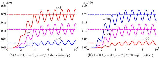
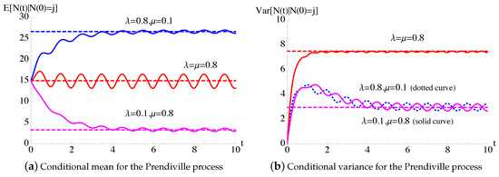
In Figure 13, the transition probabilities $p_{j,n}\left(t\right|0)$, given in (68), of the time-inhomogeneous Prendiville process, with $\lambda \left(t\right)$ given in (54), are plotted as function of t with $j=15$, $K=30$, $a=0.9$, $Q=1.0$ and for some choices of λ and μ. The dashed line indicate the steady-state probabilities $q_0$, $q_1$, $q_2$ on the left and the steady-state probabilities $q_{28}$, $q_{29}$, $q_{30}$ on the right, given in (71), of the time-homogeneous Prendiville process having ${\lambda }_n\left(t\right)=(K-n)\lambda$ and ${\mu }_n\left(t\right)=n\mu$.

Figure 13. For the Prendiville process, having ${\lambda }_n\left(t\right)=\lambda \left(t\right)(n+\nu )$ and ${\mu }_n\left(t\right)=\mu n$, with $\lambda \left(t\right)$ given in (54), the probabilities $p_{j,n}\left(t\right|0)$ are plotted as function of t with $j=15$, $K=30$, $a=0.9$, $Q=1.0$ and for some choices of λ and μ.

In Figure 14, the conditional mean and the conditional variance are plotted as function of t for $j=15$, $K=30$, $a=0.9$, $Q=1.0$ and some choices of $\lambda ,\mu$. The dashed line indicate the asymptotic mean and the asymptotic variance, given in (72), of the time-homogeneous Prendiville process.

Figure 14. For the Prendiville process of Figure 13, the conditional mean and the conditional variance (69) are plotted as function of t for $j=15$, $K=30$, $a=0.9$, $Q=1.0$ and for some choices of λ and μ.

5. Conclusions

In this paper, we have presented a detailed analysis of the time-inhomogeneous linear birth–death processes with immigration. The transition probabilities, the conditional averages and the conditional variances are determined in closed form. Specifically, in Section 2 the transition probabilities are obtained in terms of the complete Bell polynomials. Special time-inhomogeneous processes of interest in population growth models and in queuing systems are carefully analyzed in Section 3. A time-inhomogeneous linear birth–death processes with finite state-space is also taken into account in Section 4. Special attention is devoted to the cases of periodic immigration intensity functions, that play an important role in the description of the evolution of dynamic systems in various applied fields. For instance, in population dynamics they express the existence of fluctuation in the growth due to seasonal immigration or other regular environmental cycles. Various numerical computations with MATHEMATICA are performed in the cases of periodic immigration intensity functions.

We conclude by mentioning that future research will concern the analysis of the first-passage time problem for time-inhomogeneous birth–death processes with immigration through specific boundaries interpretable as the extinction level or the saturation level (carrying capacity) in population dynamics. Moreover, our investigation will be extended to the continuous approximations of the time-inhomogeneous birth–death processes with immigration. It is expected to obtain new theoretical results on stochastic time-inhomogeneous diffusion processes, restricted to the interval $(0,+\infty )$, where the state zero is a reflecting or absorbing boundary. These studies will be used to model biological, physical and chemical systems. The knowledge of the transition distributions for discrete processes and their continuous approximations will allow the determination of the first-passage densities both through analytical methods and through numerical and simulation techniques.

References

- Bailey, N.T.J. The Elements of Stochastic Processes with Applications to the Natural Sciences; John Wiley & Sons, Inc.: New York, NY, USA, 1964. [Google Scholar]
- Conolly, B. Lecture Notes on Queueing Systems; Ellis Horwood Ltd.: Chichester, NY, USA, 1975; ISBN 0470168579. [Google Scholar]
- Feldman, M.W. Mathematical Evolutionary Theory; Princeton University Press: Princeton, NJ, USA, 1989. [Google Scholar]
- Iosifescu, M.; Tautu, F. Stochastic Processes and Applications in Biology and Medicine II. Models; Springer: Berlin/Heidelberg, Germany, 1973; ISBN 978-3-642-80755-8. [Google Scholar]
- Medhi, J. Stochastic Models in Queueing Theory; Academic Press: Amsterdam, The Netherlands, 2003. [Google Scholar]
- Ricciardi, L.M. Stochastic population theory: Birth and death processes. In Mathematical Ecology; Hallam, T.G., Levin, S.A., Eds.; Springer: Berlin/Heidelberg, Germany, 1986; Volume 17, pp. 155–190. [Google Scholar]
- Thieme, H.R. Mathematics in Population Biology; Princeton University Press: Princeton, NJ, USA, 2003. [Google Scholar]
- Di Crescenzo, A.; Giorno, V.; Nobile, A.G. Constructing transient birth–death processes by means of suitable transformations. Appl. Math. Comp. 2016, 281, 152–171. [Google Scholar] [CrossRef]
- Crawford, F.W.; Suchard, M.A. Transition probabilities for general birth–death processes with applications in ecology, genetics, and evolution. J. Math. Biol. 2012, 65, 553–580. [Google Scholar] [CrossRef]
- Giorno, V.; Nobile, A.G. First-passage times and related moments for continuous-time birth–death chains. Ric. Mat. 2019, 68, 629–659. [Google Scholar] [CrossRef]
- Lenin, R.B.; Parthasarathy, P.R.; Scheinhardt, W.R.W.; van Doorn, E.A. Families of birth–death processes with similar time-dependent behaviour. J. Appl. Probab. 2000, 37, 835–849. [Google Scholar] [CrossRef]
- Tavaré, S. The birth process with immigration, and the genealogical structure of large populations. J. Math. Biol. 1987, 25, 161–168. [Google Scholar] [CrossRef]
- Crawford, F.W.; Ho, L.S.T.; Suchard, M.A. Computational methods for birth–death processes. Wiley Interdiscip. Rev. Comput. Stat. 2018, 10. [Google Scholar] [CrossRef] [PubMed]
- Di Crescenzo, A.; Giorno, V.; Krishna Kumar, B.; Nobile, A.G. M/M/1 queue in two alternating environments and its heavy traffic approximation. J. Math. Anal. Appl. 2018, 458, 973–1001. [Google Scholar] [CrossRef]
- Giorno, V.; Nobile, A.G.; Pirozzi, E. A state-dependent queueing system with asymptotic logarithmic distribution. J. Math. Anal. Appl. 2018, 458, 949–966. [Google Scholar] [CrossRef]
- Di Crescenzo, A.; Giorno, V.; Krishna Kumar, B.; Nobile, A.G. A double-ended queue with catastrophes and repairs, and a jump-diffusion approximation. Methodol. Comput. Appl. Probab. 2012, 14, 937–954. [Google Scholar] [CrossRef]
- Dharmaraja, S.; Di Crescenzo, A.; Giorno, V.; Nobile, A.G. A continuous-time Ehrenfest model with catastrophes and its jump-diffusion approximation. J. Stat. Phys. 2015, 161, 326–345. [Google Scholar] [CrossRef]
- Giorno, V.; Nobile, A.G. On a Bilateral Linear Birth and Death Process in the Presence of Catastrophe. In Computer Aided Systems Theory-EUROCAST 2013, Part I; LNCS 8111; Moreno-Diaz, R., Pichler, F., Quesada-Arencibia, A., Eds.; Springer: Berlin/Heidelberg, Germany, 2013; pp. 28–35. [Google Scholar]
- Economou, A.; Fakinos, D. Alternative approaches for the transient analysis of Markov chains with catastrophes. J. Stat. Theory Pract. 2008, 2, 183–197. [Google Scholar] [CrossRef][Green Version]
- Kapodistria, S.; Phung-Duc, T.; Resing, J. Linear birth/immigration-death process with binomial catastrophes. Prob. Eng. Inf. Sci. 2016, 30, 79–111. [Google Scholar] [CrossRef]
- Branson, D. Inhomogeneous birth–death and birth–death-immigration processes and the logarithmic series distribution. Stoch. Process. Appl. 1991, 39, 131–137. [Google Scholar] [CrossRef]
- Di Crescenzo, A.; Giorno, V.; Krishna Kumar, B.; Nobile, A.G. A time-non-homogeneous double-ended queue with failures and repairs and its continuous approximation. Mathematics 2018, 6, 81. [Google Scholar] [CrossRef]
- Giorno, V.; Nobile, A.G.; Spina, S. On some time non-homogeneous queueing systems with catastrophes. Appl. Math. Comput. 2014, 245, 220–234. [Google Scholar] [CrossRef]
- Giveen, S.M. A taxicab problem with time-dependent arrival rates. SIAM Rev. 1963, 5, 119–127. [Google Scholar] [CrossRef]
- Zeifman, A.; Satin, Y.; Korolev, V.; Shorgin, S. On truncations for weakly ergodic inhomogeneous birth and death processes. Int. J. Appl. Math. Comput. Sci. 2014, 24, 503–518. [Google Scholar] [CrossRef]
- Satin, Y.; Zeifman, A.; Kryukova, A. On the rate of convergence and limiting characteristics for a nonstationary queueing model. Mathematics 2019, 7, 678. [Google Scholar] [CrossRef]
- Giorno, V.; Nobile, A.G. On a class of birth–death processes with time-varying intensity functions. Appl. Math. Comput. 2020, 379. [Google Scholar] [CrossRef]
- Dong, J.; Whitt, W. Using a birth-and-death process to estimate the steady-state distribution of a periodic queue. Naval Res. Logist. 2015, 62, 664–685. [Google Scholar] [CrossRef]
- Giorno, V.; Nobile, A.G.; Ricciardi, L.M. On some time-nonhomogeneous diffusion approximations to queueing systems. Adv. Appl. Prob. 1987, 19, 974–994. [Google Scholar] [CrossRef]
- Whitt, W. The steady-state distribution of the Mt/M/∞ queue with sinusoidal arrival rate function. Oper. Res. Lett. 2014, 42, 311–318. [Google Scholar] [CrossRef]
- Bodrova, A.; Chechkin, A.V.; Cherstvy, A.G.; Metzler, R. Quantifying non-ergodic dynamics of force-free granular gases. Phys. Chem. Chem. Phys. 2015, 17, 21791–21798. [Google Scholar] [CrossRef]
- Bodrova, A.S.; Chechkin, A.V.; Cherstvy, A.G.; Safdari, H.; Sokolov, I.M.; Metzler, R. Underdamped scaled Brownian motion: (non-)existence of the overdamped limit in anomalous diffusion. Sci. Rep. 2016, 6, 30520. [Google Scholar] [CrossRef] [PubMed]
- Karlin, S.; McGregor, J. Linear growth, birth and death processes. J. Math. Mech. 1958, 7, 643–662. [Google Scholar] [CrossRef]
- Konno, H. On the exact solution of a generalized Polya process. Adv. Math. Phys. 2010, 504267. [Google Scholar] [CrossRef]
- Kendall, D.G. On the generalized “birth-and-death” process. Ann. Math. Stat. 1948, 19, 1–15. [Google Scholar] [CrossRef]
- Van Den Broek, J.; Heesterbeek, H. Nonhomogeneous birth and death models for epidemic outbreak data. Biostatistics 2007, 8, 453–467. [Google Scholar] [CrossRef] [PubMed]
- Tavaré, S. The linear birth–death process: An inferential retrospective. Adv. Appl. Probab. 2018, 50, 253–269. [Google Scholar] [CrossRef]
- Ohkubo, J. Karlin-McGregor-like formula in a simple time-inhomogeneous birth–death process. J. Phys. A Math. Theor. 2014, 47, 405001. [Google Scholar] [CrossRef]
- Ohkubo, J. Lie algebraic discussions for time-inhomogeneous linear birth–death processes with immigration. J. Stat. Phys. 2014, 157, 380–391. [Google Scholar] [CrossRef][Green Version]
- Di Crescenzo, A.; Nobile, A.G. Diffusion approximation to a queueing system with time dependent arrival and service rates. Queueing Syst. 1995, 19, 41–62. [Google Scholar] [CrossRef]
- Zheng, Q. Note on the non-homogeneous Prendiville process. Math. Biosci. 1998, 148, 1–5. [Google Scholar] [CrossRef]
- Giorno, V.; Nobile, A.G.; Spina, S. Some Remarks on the Prendiville Model in the Presence of Jumps. In Computer Aided Systems Theory—EUROCAST 2019; Moreno-Díaz, R., Pichler, F., Quesada-Arencibia, A., Eds.; LNCS 12013; Springer: Cham, Switzerland, 2020; pp. 150–157. [Google Scholar]
- Giorno, V.; Negri, C.; Nobile, A.G. A solvable model for a finite capacity queueing system. J. Appl. Prob. 1985, 22, 903–911. [Google Scholar] [CrossRef]
- Williams, W.E. Partial Differential Equations; Clarendon Press: Oxford, UK, 1980. [Google Scholar]
- Comtet, L. Advanced Combinatorics: The Art of Finite and Infinite Expansions; D. Reidel Publishing Company: Boston, MA, USA, 1974. [Google Scholar]
© 2020 by the authors. Licensee MDPI, Basel, Switzerland. This article is an open access article distributed under the terms and conditions of the Creative Commons Attribution (CC BY) license (http://creativecommons.org/licenses/by/4.0/).