Asymptotic Diffusion Analysis of Multi-Server Retrial Queue with Hyper-Exponential Service

Abstract

A multi-server retrial queue with a hyper-exponential service time is considered in this paper. The study is performed by the method of asymptotic diffusion analysis under the condition of long delay in orbit. On the basis of the constructed diffusion process, we obtain approximations of stationary probability distributions of the number of customers in orbit and the number of busy servers. Using simulations and numerical analysis, we estimate the accuracy and applicability area of the obtained approximations.

1. Introduction

Nowadays, retrial queues (RQ) are very popular mathematical models of various real systems. These may be call centers [1,2] where a calling customer, if he or she find all operators busy, tries to make a new call again after some (random) time. In the case of modeling of data transmission via TCP [3] if a data packet is lost or corrupted, the packet should be retransmitted after certain time. In cellular mobile networks, more complex models of retrial queues are used (see [4,5]). Furthermore, we see great opportunities in using multi-server retrial queues for modeling and design data processing systems with high-intensity data flows [6,7]. These are not only fields where retrial queues may be applied (e.g., survey [8]).

A retrial queue is a such queueing system with limited number of servers where customers that arrived and do not find a free server are not lost, but go to special ‘waiting’ state, or are moved to special buffer (orbit) for waiting. In the orbit, the customers are not organizing in a queue (e.g., first come, first served (FCFS)), but wait for a random time and then try to obtain the service again. There are a great number of RQs modifications considered by various authors—From ordinary single-server or multi-server systems to retrial queues with several orbits, priorities, collisions and so on. Detail information about retrial queue models, their analysis and applications you may find in surveys [8,9,10,11,12] and others.

Most of the authors consider single-line retrial queues and or retrial queues with exponentially distributed service time. In this paper, we consider a multi-line retrial queue with hyper-exponential service time, but we hold in mind a such model with arbitrary distributed service time as the aim for future work.

Unfortunately, exact analytical solutions for retrial queues may be derived in very rare cases. Due to this, the most authors use numerical methods, approximations or even simulation methods to study more complex retrial queues [13,14,15,16,17]. This also applies to multi-server models [16] including systems with non-exponential service time [13].

Traditionally, we study retrial queues under various asymptotic conditions such as heavy load or long delay [18,19,20,21]. In these studies we and our colleagues obtained approximations for stationary probability distributions of the number of customers in the orbit that are applicable in appropriate conditions. Unlike these previous works, in this paper, we apply a new approach—The asymptotic diffusion method [22]—To perform more detailed and accurate analysis of the model. This will give more precise approximations and wider areas of their applicability.

The rest of the paper is organized as follows. In Section 2, we describe in detail a mathematical model of the considered retrial queue and derive balance equations. In Section 3 and Section 4, we perform asymptotic analysis of obtained equations under condition of long delay in the orbit. In Section 5, we introduce the method of asymptotic diffusion analysis and construct a diffusion process which is used in Section 6 to build approximations for steady-state probability distributions of the number of busy servers and the number of customers in the orbit. Using simulations and numerical experiments, we determine the applicability area of suggested approximations in Section 7.

2. Mathematical Model

Consider a retrial queue with N servers and Poisson arrivals with intensity $\mathsf{\lambda }$. Service times are independent and identically distributed as hyper-exponential variables with cumulative distribution function

$$B\left(x\right)=q_1\left(1-e^{-{\mathsf{\mu }}_{1}x}\right)+q_2\left(1-e^{-{\mathsf{\mu }}_{2}x}\right),$$

(1)

where ${\mathsf{\mu }}_1,{\mathsf{\mu }}_2>0$, $0<q_1<1$, and $q_1+q_2=1$.

When a customer arrives, if there is a free server the customer moves to it for service, otherwise the customer goes to the orbit and stays there during random period exponentially distributed with parameter $\mathsf{\sigma }$. After this period the customer tries to get a service again according to the described algorithm.

Let us denote the number of busy servers at the moment t by $n\left(t\right)\in \{0,1,\dots ,N\}$, and the number of customers in the orbit by $i\left(t\right)\in \{0,1,2\dots \}$. The problem is to find steady-state probability distribution of the two-dimensional process $\left\{n\right(t),i(t\left)\right\}$ that we denote by

$$P(n,i)=\mathrm{P}\left\{n\right(t)=n,i(t)=i\}$$

for all $n\in \{0,1,\dots ,N\}$ and $i\in \{0,1,2\dots \}$ independently of t.

To solve the problem, let us consider the stochastic process $\{n_1\left(t\right),n_2\left(t\right),i\left(t\right)\}$, where $n_1\left(t\right)$ and $n_2\left(t\right)$ are the numbers of busy servers that realizes the service time of the first phase or the second phase respectively. The process is Markovian, hence we can write balance equations for its probability distribution

$$P(n_1,n_2,i,t)=\mathrm{P}\{n_1\left(t\right)=n_1,n_2\left(t\right)=n_2,i\left(t\right)=i\},$$

where $0\le n_1+n_2\le N$, $i\in \{0,1,2\dots \}$. So, we can write differential equations

$$\begin{array}{c}\begin{array}{c}\frac{\partial P(n_1,n_2,i,t)}{\partial t}=-(\mathsf{\lambda }+n_1{\mathsf{\mu }}_1+n_2{\mathsf{\mu }}_2+i\mathsf{\sigma })P(n_1,n_2,i,t)+q_1\mathsf{\lambda }P(n_1-1,n_2,i,t)+q_2\mathsf{\lambda }P(n_1,n_2-1,i,t)\\ +q_1(i+1)\mathsf{\sigma }P(n_1-1,n_2,i+1,t)+q_2(i+1)\mathsf{\sigma }P(n_1,n_2-1,i+1,t)\\ +(n_1+1){\mathsf{\mu }}_{1}P\left((n_1+1,n_2,i,t)\right)+(n_2+1){\mathsf{\mu }}_{2}P(n_1,n_2+1,i,t)\end{array}\end{array}$$

(2)

for the case $n_1+n_2\le N-1$, and

$$\begin{array}{c}\frac{\partial P(n_1,n_2,i,t)}{\partial t}=-(\mathsf{\lambda }+n_1{\mathsf{\mu }}_1+n_2{\mathsf{\mu }}_2)P(n_1,n_2,i,t)\\ +q_1\mathsf{\lambda }P(n_1-1,n_2,i,t)+q_2\mathsf{\lambda }P(n_1,n_2-1,i,t)+\mathsf{\lambda }P(n_1,n_2,i-1,t)\\ +q_1(i+1)\mathsf{\sigma }P(n_1-1,n_2,i+1,t)+q_2(i+1)\mathsf{\sigma }P(n_1,n_2-1,i+1,t)\end{array}$$

(3)

for the case $n_1+n_2=N$.

Let us introduce partial characteristic functions

$$H(n_1,n_2,u,t)={\displaystyle \sum _{i=0}^{\infty }}{e}^{jui}P(n_1,n_2,i,t),$$

where $j=\sqrt{-1}$. Then we can rewrite the system of balance Equations (2)–(3) as follows:

$$\begin{array}{c}\begin{array}{c}\frac{\partial H(n_1,n_2,u,t)}{\partial t}=-(\mathsf{\lambda }+n_1{\mathsf{\mu }}_1+n_2{\mathsf{\mu }}_2)H(n_1,n_2,u,t)+q_1\mathsf{\lambda }H(n_1-1,n_2,u,t)+q_2\mathsf{\lambda }H(n_1,n_2-1,u,t)\\ +(n_1+1){\mathsf{\mu }}_{1}H(n_1+1,n_2,u,t)+(n_2+1){\mathsf{\mu }}_{2}H(n_1,n_2+1,u,t)\\ -j\mathsf{\sigma }{q}_1{e}^{-ju}\frac{\partial H(n_1-1,n_2,u,t)}{\partial u}-j\mathsf{\sigma }{q}_2{e}^{-ju}\frac{\partial H(n_1,n_2-1,u,t)}{\partial u}+j\mathsf{\sigma }\frac{\partial H(n_1,n_2,u,t)}{\partial u}\end{array}\end{array}$$

(4)

for $n_1+n_2\le N-1$, and

$$\begin{array}{c}\frac{\partial H(n_1,n_2,u,t)}{\partial t}=-(\mathsf{\lambda }+n_1{\mathsf{\mu }}_1+n_2{\mathsf{\mu }}_2)H(n_1,n_2,u,t)\\ +q_1\mathsf{\lambda }H(n_1-1,n_2,u,t)+q_2\mathsf{\lambda }H(n_1,n_2-1,u,t)+\mathsf{\lambda }{e}^{ju}H(n_1,n_2,u,t)\\ -j\mathsf{\sigma }{q}_1{e}^{-ju}\frac{\partial H(n_1-1,n_2,u,t)}{\partial u}-j\mathsf{\sigma }{q}_2{e}^{-ju}\frac{\partial H(n_1,n_2-1,u,t)}{\partial u}\end{array}$$

(5)

for $n_1+n_2=N$.

Let us use linear finite difference operators $\mathbf{A},\mathbf{B},{\mathbf{I}}_0,{\mathbf{I}}_1$ to rewrite the system Equations (4) and (5) in a compact form. Then using notation $\mathbf{H}(u,t)$ for $(N+1)\times (N+1)$ matrix function with indexes $n_1,n_2=0,\dots ,N$ and entries equal to $H(n_1,n_2,u,t)$ for $n_1+n_2\le N$ or zero otherwise, we can rewrite Equations (4) and (5) as follows:

$$\frac{\partial \mathbf{H}(u,t)}{\partial t}=\mathbf{H}(u,t)\left(\mathbf{A}+e^{ju}\mathbf{B}\right)+j\mathsf{\sigma }\frac{\partial \mathbf{H}(u,t)}{\partial u}\left({\mathbf{I}}_0-e^{-ju}{\mathbf{I}}_1\right).$$

(6)

Here

$$\begin{array}{c}\mathbf{H}(u,t)\mathbf{A}=-(\mathsf{\lambda }+n_1{\mathsf{\mu }}_1+n_2{\mathsf{\mu }}_2)H(n_1,n_2,u,t)+q_1\mathsf{\lambda }H(n_1-1,n_2,u,t)+q_2\mathsf{\lambda }H(n_1,n_2-1,u,t)\\ +\psi (n_1+n_2,N)\left[(n_1+1){\mathsf{\mu }}_{1}H(n_1+1,n_2,u,t)+(n_2+1){\mathsf{\mu }}_{2}H(n_1,n_2+1,u,t)\right],\end{array}$$

$$\mathbf{H}(u,t)\mathbf{B}=\left[1-\psi (n_1+n_2,N)\right]\mathsf{\lambda }H(n_1,n_2,u,t),$$

$$\mathbf{H}(u,t){\mathbf{I}}_0=\psi (n_1+n_2,N)H(n_1,n_2,u,t),$$

$$\mathbf{H}(u,t){\mathbf{I}}_1=q_{1}H(n_1-1,n_2,u,t)+q_{2}H(n_1,n_2-1,u,t),$$

where indicator $\psi (n_1+n_2,N)$ is defined as follows:

$$\psi (n_1+n_2,N)=\left\{\begin{array}{c}1,\mathrm{if} 0\le n_1+n_2<N,\hfill \\ 0,\mathrm{otherwise}:n_1+n_2=N.\hfill \end{array}\right.$$

We write these operators on the right hand of matrix function affected by them similar to notations of matrix operations.

Let us denote summing operator by $\mathbf{E}$. Applying this operator on Equation (6) and taking into account that

$$(\mathbf{A}+\mathbf{B})\mathbf{E}=\mathbf{0}$$

(7)

and

$$({\mathbf{I}}_0-{\mathbf{I}}_1)\mathbf{E}=\mathbf{0},$$

(8)

we obtain the following scalar equation:

$$\frac{\partial \mathbf{H}(u,t)}{\partial t}\mathbf{E}=\left(e^{ju}-1\right)\left\{\mathbf{H}(u,t)\mathbf{B}+j\mathsf{\sigma }{e}^{-ju}\frac{\partial \mathbf{H}(u,t)}{\partial u}{\mathbf{I}}_0\right\}\mathbf{E}.$$

(9)

It will be an additional equation to the system Equation (6).

3. First Stage of the Asymptotic Analysis

System of Equations (6) and (9) can not be solved in a direct way, so, we will solve it under asymptotic condition of long delay in the orbit: $\mathsf{\sigma }\to 0$.

Denoting $\mathsf{\sigma }=\epsilon$, we make the following substitutions in system Equations (6) and (9):

$$\tau =t\epsilon ,u=\epsilon w,\mathbf{H}(u,t)=\mathbf{F}(w,\tau ,\epsilon ).$$

(10)

We obtain

$$\epsilon \frac{\partial \mathbf{F}(w,\tau ,\epsilon )}{\partial \tau }=\mathbf{F}(w,\tau ,\epsilon )\left(\mathbf{A}+e^{j\epsilon w}\mathbf{B}\right)+j\frac{\partial \mathbf{F}(w,\tau ,\epsilon )}{\partial w}\left({\mathbf{I}}_0-e^{-j\epsilon w}{\mathbf{I}}_1\right),$$

(11)

$$\epsilon \frac{\partial \mathbf{F}(w,\tau ,\epsilon )}{\partial \tau }\mathbf{E}=\left(e^{j\epsilon w}-1\right)\left\{\mathbf{F}(w,\tau ,\epsilon )\mathbf{B}\mathbf{E}+j{e}^{-j\epsilon w}\frac{\partial \mathbf{F}(w,\tau ,\epsilon )}{\partial w}{\mathbf{I}}_0\mathbf{E}\right\}.$$

(12)

We will solve system Equations (11) and (12) under asymptotic condition $\epsilon \to 0$.

Let $x=x\left(\tau \right)=\underset{\epsilon \to 0}{lim}\mathrm{E}\left\{\epsilon i\left(\tau \right)\right\}$ be a scalar function which determines the average number of customers in the orbit normalized by $\epsilon =\mathsf{\sigma }$ asymptotically for $\epsilon \to 0$. Denote probabilities of the number of busy servers working at the first phase ($n_1$) or second phase ($n_2$) of given hyper-exponential distribution of service time by $R(n_1,n_2,x)$ for $n_1,n_2=0,\dots ,N$ and $n_1+n_2\le N$. Let $\mathbf{R}\left(x\right)$ be $(N+1)\times (N+1)$ left-top triangle matrix with entries equal to $R(n_1,n_2,x)$ for $n_1+n_2\le N$ and others equal to zero.

Theorem 1.

Under asymptotic condition $\epsilon \to 0$, probabilities $R(n_1,n_2,x)$ are determined by expressions

$$\begin{array}{c}R(n_1,n_2,x)=\frac{{\rho }_1{\left(x\right)}^{n_1}}{n_1!}·\frac{{\rho }_2{\left(x\right)}^{n_2}}{n_2!}R(0,0,x),\\ R(0,0,x)=1/{\displaystyle \sum _{n_1+n_2\le N}}\frac{{\rho }_1{\left(x\right)}^{n_1}}{n_1!}·\frac{{\rho }_2{\left(x\right)}^{n_2}}{n_2!},\end{array}$$

(13)

where

$${\rho }_1\left(x\right)=q_1\frac{(\mathsf{\lambda }+x)}{{\mathsf{\mu }}_1},{\rho }_2\left(x\right)=q_2\frac{(\mathsf{\lambda }+x)}{{\mathsf{\mu }}_2},$$

(14)

and $x=x\left(\tau \right)$ is a solution of the ordinary differential equation

$$x^{\prime }\left(\tau \right)=\mathbf{R}\left(x\right)\left(\mathbf{B}-x\left(\tau \right){\mathbf{I}}_0\right)\mathbf{E}.$$

(15)

Proof. 

Making asymptotic transition $\epsilon \to 0$ in Equations (11) and (12) and denoting $\underset{\epsilon \to 0}{lim}\mathbf{F}(w,\tau ,\epsilon )=\mathbf{F}(w,\tau )$, we derive

$$\begin{array}{c}\mathbf{F}(w,\tau )(\mathbf{A}+\mathbf{B})+j\frac{\partial \mathbf{F}(w,\tau )}{\partial w}({\mathbf{I}}_0-{\mathbf{I}}_1)=0,\\ \frac{\partial \mathbf{F}(w,\tau )}{\partial \tau }\mathbf{E}=jw\left\{\mathbf{F}(w,\tau )\mathbf{B}\mathbf{E}+j\frac{\partial \mathbf{F}(w,\tau )}{\partial w}{\mathbf{I}}_0\mathbf{E}\right\}.\end{array}$$

(16)

Let us find a solution of system Equation (16) in the form

$$\mathbf{F}(w,\tau )=\mathbf{R}\left(x\right)e^{jwx\left(\tau \right)}.$$

(17)

Substituting Equation (17) into Equation (16), we derive

$$\mathbf{R}\left(x\right)\left\{\mathbf{A}+\mathbf{B}-x\left(\tau \right)\left({\mathbf{I}}_0-{\mathbf{I}}_1\right)\right\}=0,$$

(18)

$$x^{\prime }\left(\tau \right)=\mathbf{R}\left(x\right)\left(\mathbf{B}-x\left(\tau \right){\mathbf{I}}_0\right)\mathbf{E}.$$

(19)

So, Equation (18) is a homogeneous system of linear equations for $R(n_1,n_2,x)$ which solution depends on $x\left(\tau \right)$. Equation (19) (that coincides with Equation (15)) is an ordinary differential equation of the first order for function $x\left(\tau \right)$. So, we can find a solution of Equation (18) and substitute it into Equation (19).

Let us solve system Equation (18). To do this, we rewrite matrix Equation (18) in the form of the following homogeneous system of linear equations:

$$\begin{array}{c}{q}_1(\mathsf{\lambda }+x)R(n_1-1,n_2,x)+q_2(\mathsf{\lambda }+x)R(n_1,n_2-1,x)-(\mathsf{\lambda }+x+n_1{\mathsf{\mu }}_1+n_2{\mathsf{\mu }}_2)R(n_1,n_2,x)\\ +(n_1+1){\mathsf{\mu }}_{1}R(n_1+1,n_2,x)+(n_2+1){\mathsf{\mu }}_{2}R(n_1,n_2+1,x)=0\end{array}$$

for $n_1+n_2\le N-1$, and

$$q_1(\mathsf{\lambda }+x)R(n_1-1,n_2,x)+q_2(\mathsf{\lambda }+x)R(n_1,n_2-1,x)-(n_1{\mathsf{\mu }}_1+n_2{\mathsf{\mu }}_2)R(n_1,n_2,x)=0$$

for $n_1+n_2=N$. Substituting here expressions Equations (13) and (14), we obtain true identities. So, the theorem is proved. □

Let us denote

$$a\left(x\right)=\mathbf{R}\left(x\right)\left(\mathbf{B}-x\left(\tau \right){\mathbf{I}}_0\right)\mathbf{E}.$$

(20)

Corollary 1.

Let

$$r\left(x\right)={\displaystyle \sum _{n_1+n_2=N}}R(n_1,n_2,x),$$

(21)

then function $a\left(x\right)$ may be written in the form

$$a\left(x\right)=(\mathsf{\lambda }+x(\tau \left)\right)r\left(x\right)-x\left(\tau \right)$$

(22)

Proof. 

From Equation (20) we derive

$$\begin{array}{c}a\left(x\right)=\mathbf{R}\left(x\right)\left(\mathbf{B}-x\left(\tau \right){\mathbf{I}}_0\right)\mathbf{E}=a(\mathbf{R}\left(x\right)\mathbf{B}\mathbf{E}-x\left(\tau \right)\mathbf{R}\left(x\right){\mathbf{I}}_0\mathbf{E}\\ =\mathsf{\lambda }{\displaystyle \sum _{n_1+n_2=N}}R(n_1,n_2,x)-x{\displaystyle \sum _{n_1+n_2\le N-1}}R(n_1,n_2,x)\\ =\mathsf{\lambda }{\displaystyle \sum _{n_1+n_2=N}}R(n_1,n_2,x)-x\left({\displaystyle \sum _{n_1+n_2\le N}}R(n_1,n_2,x)-{\displaystyle \sum _{n_1+n_2=N}}R(n_1,n_2,x)\right)\\ =(\mathsf{\lambda }+x){\displaystyle \sum _{n_1+n_2=N}}R(n_1,n_2,x)-x{\displaystyle \sum _{n_1+n_2\le N}}R(n_1,n_2,x).\end{array}$$

Taking into account that ${\displaystyle \sum _{n_1+n_2\le N}}R(n_1,n_2,x)=1$ and using notation Equation (21), we obtain Equation (22). □

4. Second Stage of the Asymptotic Analysis

Taking into account that characteristic function of process $\frac{1}{\mathsf{\sigma }}x\left(\mathsf{\sigma }t\right)$ of the normalized number of customers in the orbit has form $exp\left\{jwx\right(\tau \left)\right\}$ (see Equation (17)), let us make the following substitution in system Equation (9):

$$\mathbf{H}(u,t)=e^{j\frac{u}{\mathsf{\sigma }}x\left(\mathsf{\sigma }t\right)}{\mathbf{H}}^{\left(1\right)}(u,t).$$

(here ${\mathbf{H}}^{\left(1\right)}(u,t)\mathbf{E}$ is characteristic function of centered process $i\left(t\right)-\frac{1}{\mathsf{\sigma }}x\left(\mathsf{\sigma }t\right)$). Then we obtain the system

$$\begin{array}{c}\frac{\partial {\mathbf{H}}^{\left(1\right)}(u,t)}{\partial t}+ju{x}^{\prime }\left(\mathsf{\sigma }t\right){\mathbf{H}}^{\left(1\right)}(u,t)={\mathbf{H}}^{\left(1\right)}(u,t)\left(\mathbf{A}+e^{ju}\mathbf{B}\right)\\ +j\mathsf{\sigma }\left[\frac{j}{\mathsf{\sigma }}x\left(\mathsf{\sigma }t\right){\mathbf{H}}^{\left(1\right)}(u,t)+\frac{\partial {\mathbf{H}}^{\left(1\right)}(u,t)}{\partial u}\right]\left({\mathbf{I}}_0-e^{-ju}{\mathbf{I}}_1\right),\\ \left[\frac{\partial {\mathbf{H}}^{\left(1\right)}(u,t)}{\partial u}+ju{x}^{\prime }\left(\mathsf{\sigma }t\right){\mathbf{H}}^{\left(1\right)}(u,t)\right]\mathbf{E}\\ =\left(e^{ju}-1\right)\left\{{\mathbf{H}}^{\left(1\right)}(u,t)\mathbf{BE}+j\mathsf{\sigma }{e}^{-ju}\left[\frac{j}{\mathsf{\sigma }}x\left(\mathsf{\sigma }t\right){\mathbf{H}}^{\left(1\right)}(u,t)+\frac{\partial {\mathbf{H}}^{\left(1\right)}(u,t)}{\partial u}\right]{\mathbf{I}}_0\mathbf{E}\right\}.\end{array}$$

(23)

Taking into account notation Equation (20), we can rewrite this system in the form

$$\begin{array}{c}\frac{\partial {\mathbf{H}}^{\left(1\right)}(u,t)}{\partial t}+jua\left(x\right){\mathbf{H}}^{\left(1\right)}(u,t)={\mathbf{H}}^{\left(1\right)}(u,t)\left[\mathbf{A}+e^{ju}\mathbf{B}-x\left({\mathbf{I}}_0-e^{-ju}{\mathbf{I}}_1\right)\right]\\ +j\mathsf{\sigma }\frac{\partial {\mathbf{H}}^{\left(1\right)}(u,t)}{\partial u}\left({\mathbf{I}}_0-e^{-ju}{\mathbf{I}}_1\right),\\ \frac{\partial {\mathbf{H}}^{\left(1\right)}(u,t)}{\partial u}\mathbf{E}+jua\left(x\right){\mathbf{H}}^{\left(1\right)}(u,t)\mathbf{E}\\ =\left(e^{ju}-1\right)\left[{\mathbf{H}}^{\left(1\right)}(u,t)\left(\mathbf{B}-e^{-ju}x{\mathbf{I}}_0\right)+e^{-ju}j\mathsf{\sigma }\frac{\partial {\mathbf{H}}^{\left(1\right)}(u,t)}{\partial u}{\mathbf{I}}_0\right]\mathbf{E}.\end{array}$$

(24)

Denoting $\mathsf{\sigma }={\epsilon }^2$ and making the following substitutions in Equation (24)

$$\tau =t{\epsilon }^2,u=\epsilon w,{\mathbf{H}}^{\left(1\right)}(u,t)={\mathbf{F}}^{\left(1\right)}(w,\tau ,\epsilon ),$$

(25)

we obtain system of differential equations

$$\begin{array}{c}{\epsilon }^2\frac{\partial {\mathbf{F}}^{\left(1\right)}(w,\tau ,\epsilon )}{\partial \tau }+j\epsilon wa\left(x\right){\mathbf{F}}^{\left(1\right)}(w,\tau ,\epsilon )={\mathbf{F}}^{\left(1\right)}(w,\tau ,\epsilon )\left[\mathbf{A}+e^{j\epsilon w}\mathbf{B}-x\left({\mathbf{I}}_0-e^{-j\epsilon w}{\mathbf{I}}_1\right)\right]\\ +j\epsilon \frac{\partial {\mathbf{F}}^{\left(1\right)}(w,\tau ,\epsilon )}{\partial w}\left({\mathbf{I}}_0-e^{-j\epsilon w}{\mathbf{I}}_1\right),\\ {\epsilon }^2\frac{\partial {\mathbf{F}}^{\left(1\right)}(w,\tau ,\epsilon )}{\partial \tau }\mathbf{E}+j\epsilon wa\left(x\right){\mathbf{F}}^{\left(1\right)}(w,\tau ,\epsilon )\mathbf{E}\\ =\left(e^{j\epsilon w}-1\right)\left[{\mathbf{F}}^{\left(1\right)}(w,\tau ,\epsilon )\left(\mathbf{B}-e^{-j\epsilon w}x{\mathbf{I}}_0\right)+e^{-j\epsilon w}j\epsilon \frac{\partial {\mathbf{F}}^{\left(1\right)}(w,\tau ,\epsilon )}{\partial w}{\mathbf{I}}_0\right]\mathbf{E}.\end{array}$$

(26)

Let us denote

$$\underset{\epsilon \to 0}{lim}{\mathbf{F}}^{\left(1\right)}(w,\tau ,\epsilon )={\mathbf{F}}^{\left(1\right)}(w,\tau ),\underset{\epsilon \to 0}{lim}\frac{\partial {\mathbf{F}}^{\left(1\right)}(w,\tau ,\epsilon )}{\partial \tau }=\frac{\partial {\mathbf{F}}^{\left(1\right)}(w,\tau )}{\partial \tau },\underset{\epsilon \to 0}{lim}\frac{\partial {\mathbf{F}}^{\left(1\right)}(w,\tau ,\epsilon )}{\partial w}=\frac{\partial {\mathbf{F}}^{\left(1\right)}(w,\tau )}{\partial w}.$$

We can prove the following theorem.

Theorem 2.

Function ${\mathbf{F}}^{\left(1\right)}(w,\tau )$ has the following form:

$${\mathbf{F}}^{\left(1\right)}(w,\tau )=\mathsf{\Phi }(w,\tau )\mathbf{R}\left(x\right),$$

(27)

where non-zero entries $R(n_1,n_2,x)$ of matrix $\mathbf{R}\left(x\right)$ are determined by Theorem 1, and scalar function $\mathsf{\Phi }(w,\tau )$ is a solution of differential equation

$$\frac{\partial \mathsf{\Phi }(w,\tau )}{\partial \tau }=a^{\prime }\left(x\right)w\frac{\partial \mathsf{\Phi }(w,\tau )}{\partial w}+b\left(x\right)\frac{{\left(jw\right)}^2}{2}\mathsf{\Phi }(w,\tau ).$$

(28)

Here function $a\left(x\right)$ is determined by Equation (20), $b\left(x\right)$ has the form

$$b\left(x\right)=a\left(x\right)+2\mathbf{g}\left(x\right)\left(\mathbf{B}-x{\mathbf{I}}_0\right)\mathbf{E}+2x\mathbf{R}\left(x\right){\mathbf{I}}_0\mathbf{E},$$

(29)

and top-left triangle matrix $\mathbf{g}\left(\mathbf{x}\right)$ is determined by the following system of equations:

$$\begin{array}{c}\mathbf{g}\left(x\right)\left[\mathbf{A}+\mathbf{B}+x\left({\mathbf{I}}_1-{\mathbf{I}}_0\right)\right]=a\left(x\right)\mathbf{R}\left(x\right)+\mathbf{R}\left(x\right)\left(x{\mathbf{I}}_1-\mathbf{B}\right),\\ \mathbf{g}\left(x\right)\mathbf{E}=0.\end{array}$$

(30)

Proof. 

Let us write only the members of the first equation of system Equation (26) that contains only zero or the first order of $\epsilon$:

$$\begin{array}{c}j\epsilon wa\left(x\right){\mathbf{F}}^{\left(1\right)}(w,\tau ,\epsilon )={\mathbf{F}}^{\left(1\right)}(w,\tau ,\epsilon )\left[\mathbf{A}+\mathbf{B}+j\epsilon w\mathbf{B}-x\left({\mathbf{I}}_0-{\mathbf{I}}_1-j\epsilon w{\mathbf{I}}_1\right)\right]\\ +j\epsilon \frac{\partial {\mathbf{F}}^{\left(1\right)}(w,\tau ,\epsilon )}{\partial w}\left({\mathbf{I}}_0-{\mathbf{I}}_1\right)+O\left({\epsilon }^2\right).\end{array}$$

(31)

Solution of this equation we write in the form

$${\mathbf{F}}^{\left(1\right)}(w,\tau ,\epsilon )=\mathsf{\Phi }(w,\tau )\left[\mathbf{R}\left(x\right)+j\epsilon w\mathbf{f}\left(x\right)\right]+O\left({\epsilon }^2\right),$$

(32)

where $\mathsf{\Phi }(w,\tau )$ and $\mathbf{f}\left(x\right)$ are some scalar and matrix functions whose expressions we will obtain later. Substituting this expression into Equation (31), we derive

$$\begin{array}{c}j\epsilon wa\left(x\right)\mathsf{\Phi }(w,\tau )\mathbf{R}\left(x\right)=\mathsf{\Phi }(w,\tau )\{\mathbf{R}\left(x\right)\left[\mathbf{A}+\mathbf{B}-x\left({\mathbf{I}}_0-{\mathbf{I}}_1\right)\right]\\ +j\epsilon w\left[\mathbf{f}\left(x\right)\left(\mathbf{A}+\mathbf{B}-x({\mathbf{I}}_0-{\mathbf{I}}_1)\right)\right]\}\\ +j\epsilon \frac{\partial \mathsf{\Phi }(w,\tau )}{\partial w}\mathbf{R}\left(x\right)\left({\mathbf{I}}_0-{\mathbf{I}}_1\right)+O\left({\epsilon }^2\right).\end{array}$$

(33)

Taking into account Equation (20), dividing Equation (33) by $j\epsilon w\mathsf{\Phi }(w,\tau )$ and tending $\epsilon \to 0$, we obtain

$$a\left(x\right)\mathbf{R}\left(x\right)=\mathbf{f}\left(x\right)\left[\mathbf{A}+\mathbf{B}-x\left({\mathbf{I}}_0-{\mathbf{I}}_1\right)\right]+\mathbf{R}\left(x\right)\left(\mathbf{B}-x{\mathbf{I}}_1\right)+\frac{\partial \mathsf{\Phi }(w,\tau )/\partial w}{w\mathsf{\Phi }(w,\tau )}\mathbf{R}\left(x\right)\left({\mathbf{I}}_0-{\mathbf{I}}_1\right).$$

Let us rewrite this equality in the form of non-homogeneous equation

$$\mathbf{f}\left(x\right)\left[\mathbf{A}+\mathbf{B}+x\left({\mathbf{I}}_1-{\mathbf{I}}_0\right)\right]=a\left(x\right)\mathbf{R}\left(x\right)-\mathbf{R}\left(x\right)\left(\mathbf{B}-x{\mathbf{I}}_1\right)-\frac{\partial \mathsf{\Phi }(w,\tau )/\partial w}{w\mathsf{\Phi }(w,\tau )}\mathbf{R}\left(x\right)\left({\mathbf{I}}_0-{\mathbf{I}}_1\right).$$

(34)

According to superposition principle, we can write a solution of this equation in the form

$$\mathbf{f}\left(x\right)=C\mathbf{R}\left(x\right)+\mathbf{g}\left(x\right)-\phi \left(x\right)\frac{\partial \mathsf{\Phi }(w,\tau )/\partial w}{w\mathsf{\Phi }(w,\tau )}.$$

(35)

Substituting it into Equation (34), we obtain equations

$$\phi \left(x\right)\left[\mathbf{A}+\mathbf{B}+x\left({\mathbf{I}}_1-{\mathbf{I}}_0\right)\right]=\mathbf{R}\left(x\right)\left({\mathbf{I}}_0-{\mathbf{I}}_1\right),$$

(36)

$$\mathbf{g}\left(x\right)\left[\mathbf{A}+\mathbf{B}+x\left({\mathbf{I}}_1-{\mathbf{I}}_0\right)\right]=a\left(x\right)\mathbf{R}\left(x\right)+\mathbf{R}\left(x\right)\left(x{\mathbf{I}}_1-\mathbf{B}\right).$$

(37)

Notice that Equation (37) for matrix $\mathbf{g}\left(x\right)$ coincides with the first expression of Equation (30), therefore statement Equation (30) is true (the second expression of Equation (30) will be discussed later).

Now, consider Equation (18). Let us differentiate it by x, we derive equation

$$\frac{d\mathbf{R}\left(x\right)}{dx}\left[\mathbf{A}+\mathbf{B}-x\left({\mathbf{I}}_0-{\mathbf{I}}_1\right)\right]-\mathbf{R}\left(x\right)\left({\mathbf{I}}_0-{\mathbf{I}}_1\right)=\mathbf{0}.$$

Taking into account Equation (36), we can conclude that

$$\phi \left(x\right)=\frac{d\mathbf{R}\left(x\right)}{dx},$$

(38)

where ${\displaystyle \phi \left(x\right)\mathbf{E}=\frac{d\mathbf{R}\left(x\right)}{dx}\mathbf{E}=\frac{d\left(\mathbf{R}\right(x\left)\mathbf{E}\right)}{dx}=0}$.

Matrix $\mathbf{g}\left(x\right)$ is a particular solution to non-homogeneous system Equation (37), so it should satisfy some additional condition which we choose in the form $\mathbf{g}\left(x\right)\mathbf{E}=0$ (as was declared in Equation (30)). Then solution $\mathbf{g}\left(x\right)$ of system Equation (37) is uniquely determined.

Now, let us consider the second Equation of Equation (26). We substitute expansion Equation (32) in it and write the members of derived equation including up to the second order of $\epsilon$:

$$\begin{array}{c}{\epsilon }^2\frac{\partial \mathsf{\Phi }(w,\tau )}{\partial \tau }+j\epsilon wa\left(x\right)\mathsf{\Phi }(w,\tau )\left[1+j\epsilon w\mathbf{f}\left(x\right)\right]\mathbf{E}=\\ \left[j\epsilon w+\frac{{\left(j\epsilon w\right)}^2}{2}\right]\left\{\mathsf{\Phi }(w,\tau )\left[\mathbf{R}\left(x\right)+j\epsilon w\mathbf{f}\left(x\right)\right]\left(\mathbf{B}-x{\mathbf{I}}_0+j\epsilon wx{\mathbf{I}}_0\right)+j\epsilon \frac{\partial \mathsf{\Phi }(w,\tau )}{\partial w}\mathbf{R}\left(x\right){\mathbf{I}}_0\right\}\mathbf{E}+O\left({\epsilon }^3\right).\end{array}$$

Then we derive

$$\begin{array}{c}{\epsilon }^2\frac{\partial \mathsf{\Phi }(w,\tau )}{\partial \tau }+j\epsilon wa\left(x\right)\mathsf{\Phi }(w,\tau )+{\left(j\epsilon w\right)}^{2}a\left(x\right)\mathsf{\Phi }(w,\tau )\mathbf{f}\left(x\right)\mathbf{E}=\\ \mathsf{\Phi }(w,\tau )\{j\epsilon w\mathbf{R}\left(x\right)\left[\mathbf{B}-x{\mathbf{I}}_0\right]+{\left(j\epsilon w\right)}^2\mathbf{f}\left(x\right)\left[\mathbf{B}-x{\mathbf{I}}_0\right]+{\left(j\epsilon w\right)}^2\mathbf{R}\left(x\right)x{\mathbf{I}}_0\\ +\frac{{\left(j\epsilon w\right)}^2}{2}\mathbf{R}\left(x\right)\left[\mathbf{B}-x{\mathbf{I}}_0\right]+{\left(j\epsilon w\right)}^2\frac{\partial \mathsf{\Phi }(w,\tau )/\partial w}{w}\mathbf{R}\left(x\right){\mathbf{I}}_0\}\mathbf{E}+O\left({\epsilon }^3\right).\end{array}$$

Applying Equation (20), we obtain

$$\begin{array}{c}{\epsilon }^2\frac{\partial \mathsf{\Phi }(w,\tau )}{\partial \tau }+{\left(j\epsilon w\right)}^{2}a\left(x\right)\mathsf{\Phi }(w,\tau )\mathbf{f}\left(x\right)\mathbf{E}=\\ \mathsf{\Phi }(w,\tau )\{{\left(j\epsilon w\right)}^2\mathbf{f}\left(x\right)\left[\mathbf{B}-x{\mathbf{I}}_0\right]+{\left(j\epsilon w\right)}^2\mathbf{R}\left(x\right)x{\mathbf{I}}_0+\frac{{\left(j\epsilon w\right)}^2}{2}a\left(x\right)\\ +{\left(j\epsilon w\right)}^2\frac{\partial \mathsf{\Phi }(w,\tau )/\partial w}{w}\mathbf{R}\left(x\right){\mathbf{I}}_0\}\mathbf{E}+O\left({\epsilon }^3\right).\end{array}$$

Let us divide this equation by ${\epsilon }^2$:

$$\begin{array}{c}\frac{\partial \mathsf{\Phi }(w,\tau )}{\partial \tau }=\mathsf{\Phi }(w,\tau )\{{\left(jw\right)}^2\mathbf{f}\left(x\right)\left[\mathbf{B}-x{\mathbf{I}}_0\right]+{\left(jw\right)}^2\mathbf{R}\left(x\right)x{\mathbf{I}}_0+\frac{{\left(jw\right)}^2}{2}a\left(x\right)\\ -{\left(jw\right)}^{2}a\left(x\right)\mathbf{f}\left(x\right)+{\left(jw\right)}^2\frac{\partial \mathsf{\Phi }(w,\tau )/\partial w}{w}\mathbf{R}\left(x\right){\mathbf{I}}_0\}\mathbf{E}.\end{array}$$

So, we derive

$$\begin{array}{c}\frac{\partial \mathsf{\Phi }(w,\tau )/\partial \tau }{\mathsf{\Phi }(w,\tau )}=\frac{{\left(jw\right)}^2}{2}\left\{2\left[\mathbf{f}\left(x\right)\left(\mathbf{B}-x{\mathbf{I}}_0\right)+\mathbf{R}\left(x\right)x{\mathbf{I}}_0-a\left(x\right)\mathbf{f}\left(x\right)\right]\mathbf{E}+a\left(x\right)\right\}-w\frac{\partial \mathsf{\Phi }(w,\tau )/\partial w}{\mathsf{\Phi }(w,\tau )}\mathbf{R}\left(x\right){\mathbf{I}}_0\mathbf{E}.\end{array}$$

Substituting Equation (35) here, we obtain

$$\begin{array}{c}\frac{\partial \mathsf{\Phi }(w,\tau )/\partial \tau }{\mathsf{\Phi }(w,\tau )}=\frac{{\left(jw\right)}^2}{2}\left\{2\mathbf{g}\left(x\right)\left(\mathbf{B}-x{\mathbf{I}}_0\right)\mathbf{E}+2\mathbf{R}\left(x\right)x{\mathbf{I}}_0\mathbf{E}+a\left(x\right)\right\}\\ +w\frac{\partial \mathsf{\Phi }(w,\tau )/\partial w}{\mathsf{\Phi }(w,\tau )}\left\{\phi \left(x\right)\left(\mathbf{B}-x{\mathbf{I}}_0\right)\mathbf{E}-\mathbf{R}\left(x\right){\mathbf{I}}_0\mathbf{E}\right\}.\end{array}$$

(39)

Denoting

$$b\left(x\right)=a\left(x\right)+2\mathbf{g}\left(x\right)\left(\mathbf{B}-x{\mathbf{I}}_0\right)\mathbf{E}+2x\mathbf{R}\left(x\right){\mathbf{I}}_0\mathbf{E},$$

(40)

we can rewrite Equation (39) in the form

$$\frac{\partial \mathsf{\Phi }(w,\tau )}{\partial \tau }=w\frac{\partial \mathsf{\Phi }(w,\tau )}{\partial w}\left\{\phi \left(x\right)\left(\mathbf{B}-x{\mathbf{I}}_0\right)\mathbf{E}-\mathbf{R}\left(x\right){\mathbf{I}}_0\mathbf{E}\right\}+\frac{{\left(jw\right)}^2}{2}b\left(x\right)\mathsf{\Phi }(w,\tau ).$$

(41)

Differentiating Equation (20) by x, we obtain

$$a^{\prime }\left(x\right)=\frac{\partial \mathbf{R}\left(x\right)}{\partial x}\left(\mathbf{B}-x{\mathbf{I}}_0\right)\mathbf{E}-\mathbf{R}\left(x\right){\mathbf{I}}_0\mathbf{E}.$$

(42)

Then, taking into account Equation (38) and substituting Equation (42) into Equation (41), we derive the equation

$$\frac{\partial \mathsf{\Phi }(w,\tau )}{\partial \tau }=a^{\prime }\left(x\right)w\frac{\partial \mathsf{\Phi }(w,\tau )}{\partial w}+b\left(x\right)\frac{{\left(jw\right)}^2}{2}\mathsf{\Phi }(w,\tau )$$

that coincides with Equation (28). So, the theorem is proved. □

Corollary 2.

Let $g_1\left(x\right)={\displaystyle \sum _{n_1+n_2=N}}g(n_1,n_2,x)$, $r\left(x\right)={\displaystyle \sum _{n_1+n_2=N}}R(n_1,n_2,x)$, then function $b\left(x\right)$ from Equation (40) may be written in the form

$$b\left(x\right)=a\left(x\right)+2\left[x\left(1-r\left(x\right)\right)+(\mathsf{\lambda }+x)g_1\left(x\right)\right].$$

(43)

Proof. 

Let us rewrite Equation (40) in scalar form:

$$\begin{array}{c}b\left(x\right)=a\left(x\right)+2\left[\mathsf{\lambda }{\displaystyle \sum _{n_1+n_2=N}}g(n_1,n_2,x)+x{\displaystyle \sum _{n_1+n_2\le N-1}}g(n_1,n_2,x)-x{\displaystyle \sum _{n_1+n_2\le N-1}}R(n_1,n_2,x)\right]=\\ a\left(x\right)+2\left[\mathsf{\lambda }{g}_1\left(x\right)+x\left\{1-x{\displaystyle \sum _{n_1+n_2=N}}R(n_1,n_2,x)\right\}-x\left\{{\displaystyle \sum _{n_1+n_2\le N}}g(n_1,n_2,x)-g_1\left(x\right)\right\}\right].\end{array}$$

Applying here condition $\mathbf{g}\left(x\right)\mathbf{E}=0$, we obtain Equation (43). □

In the next section, we will use obtained functions $a\left(x\right)$ and $b\left(x\right)$ as a drift and diffusion coefficients of a diffusion process which we apply to derive approximations for probability distributions under study.

5. Method of Asymptotic Diffusion Analysis

Taking into account notation $\mathsf{\sigma }={\epsilon }^2$ and substitutions Equation (25) from the previous section, we consider stochastic process

$$\sqrt{\mathsf{\sigma }}\left[i\left(\mathsf{\sigma }t\right)-\frac{1}{\mathsf{\sigma }}x\left(\mathsf{\sigma }t\right)\right]=\sqrt{\mathsf{\sigma }}\left[i\left(\tau \right)-\frac{1}{\mathsf{\sigma }}x\left(\tau \right)\right]$$

under asymptotic condition $\mathsf{\sigma }\to 0$. Here $i\left(\tau \right)$ is the number of customers in the orbit and function $x\left(\tau \right)$ is determined in the previous section as a solution of differential equation $x^{\prime }\left(\tau \right)=a\left(x\right)$. We can prove the following statement.

Lemma 1.

Asymptotic stochastic process

$$y\left(\tau \right)=\underset{\mathsf{\sigma }\to 0}{lim}\sqrt{\mathsf{\sigma }}\left[i\left(\tau \right)-\frac{1}{\mathsf{\sigma }}x\left(\tau \right)\right]$$

is a solution of stochastic differential equation

$$dy\left(\tau \right)=a^{\prime }\left(x\right)yd\tau +\sqrt{b\left(x\right)}dw\left(\tau \right)$$

(44)

that depends on continuous parameter x.

Proof. 

Consider Equation (28) with $a\left(x\right)$ and $b\left(x\right)$ determined by Equations (22) and (40). Solution of this equation determines asymptotic characteristic function for centered and normalized stochastic process ${\displaystyle \sqrt{\mathsf{\sigma }}\left\{i\left(\tau \right)-\frac{1}{\mathsf{\sigma }}x\left(\tau \right)\right\}}$ of the number $i\left(t\right)$ of customers in the orbit under condition $\mathsf{\sigma }\to 0$.

Let us make in this equation an inverse Fourier transform on argument w. Then for probability density function (p.d.f.) ${\displaystyle P(y,\tau )=\frac{\partial \mathrm{P}\left\{y\left(\tau \right)<y\right\}}{\partial y}}$ of process $y\left(\tau \right)$, we obtain the equation

$$\frac{\partial P(y,\tau )}{\partial \tau }=-\frac{\partial }{\partial y}\left\{a^{\prime }\left(x\right)yP(y,\tau )\right\}+\frac{1}{2}\frac{{\partial }^2}{\partial y^2}\left\{b\left(x\right)P(y,\tau )\right\},$$

which is the Fokker–Planck equation for p.d.f. $P(y,\tau )$. Hence, stochastic process $y\left(\tau \right)$ is a diffusion process with drift coefficient $a^{\prime }\left(x\right)y$ and diffusion coefficient $b\left(x\right)$. Therefore, process $y\left(\tau \right)$ is a solution of stochastic differential Equation (44). □

Let us consider the following stochastic process:

$$z\left(\tau \right)=x\left(\tau \right)+\epsilon y\left(\tau \right)$$

(45)

(here $\epsilon =\sqrt{\mathsf{\sigma }}$ as before.)

Lemma 2.

Stochastic process $z\left(\tau \right)$ is a solution to stochastic differential equation

$$dz\left(\tau \right)=a\left(z\right)d\tau +\sqrt{\mathsf{\sigma }b\left(z\right)}dw\left(\tau \right)$$

(46)

with a precision up to an infinitesimal of order ${\epsilon }^2$.

Proof. 

Due to $x\left(\tau \right)$ is a solution of differential equation $dx\left(\tau \right)=a\left(x\right)d\tau$ and process $y\left(\tau \right)$ satisfies Equation (44), the following equality is true:

$$dz\left(\tau \right)=d\left[x\left(\tau \right)+\epsilon y\left(\tau \right)\right]=\left[a\left(x\right)+\epsilon y{a}^{\prime }\left(x\right)\right]d\tau +\epsilon \sqrt{b\left(x\right)}dw\left(\tau \right).$$

(47)

We can represent its coefficients in the form

$$\begin{array}{c}a\left(x\right)+\epsilon y{a}^{\prime }\left(x\right)+O\left({\epsilon }^2\right)=a(x+\epsilon y)=a\left(z\right),\\ \epsilon \sqrt{b\left(x\right)}+O\left({\epsilon }^2\right)=\epsilon \sqrt{b\left(x\right)+O\left(\epsilon \right)}=\epsilon \sqrt{b(x+\epsilon y)}=\epsilon \sqrt{b\left(z\right)},\end{array}$$

and, so, we can rewrite Equation (47) as follows:

$$dz\left(\tau \right)=a\left(z\right)d\tau +\sqrt{\mathsf{\sigma }b\left(z\right)}dw\left(\tau \right)+O\left({\epsilon }^2\right).$$

It coincides with Equation (46) with a precision up to infinitesimal $O\left({\epsilon }^2\right)$. □

Suppose that the system is in steady-state regime. Consider stationary p.d.f. $s\left(z\right)$ for process $z\left(\tau \right)$:

$$s(z,\tau )=s\left(z\right)=\frac{\partial \mathrm{P}\left\{z\left(\tau \right)<z\right\}}{\partial z}.$$

Let us prove the following statement.

Theorem 3.

Stationary p.d.f. $s\left(z\right)$ of stochastic process $z\left(\tau \right)$ has the form

$$s\left(z\right)=\frac{C}{b\left(z\right)}exp\left\{\frac{2}{\mathsf{\sigma }}\underset{0}{\overset{z}{\int }}\frac{a\left(x\right)}{b\left(x\right)}dx\right\},$$

(48)

where C is a normalizing constant.

Proof. 

Due to $z\left(\tau \right)$ is a solution of stochastic differential Equation (46), the process is diffusion with drift coefficient $a\left(z\right)$ and diffusion coefficient $b\left(z\right)$. Therefore, its p.d.f. $s\left(z\right)$ is a solution of the Fokker–Planck equation

$$-\frac{\partial }{\partial z}\left\{a\left(z\right)s\left(z\right)\right\}+\frac{1}{2}\frac{{\partial }^2}{\partial z^2}\left\{\mathsf{\sigma }b\left(z\right)s\left(z\right)\right\}=0.$$

This equation is an ordinary differential equation of the second order. Solving it and taking into account normalization condition and boundary condition $s(\infty )=0$, we obtain Equation (48). The theorem is proved. □

6. Approximations of the Stationary Distributions

Consider matrix characteristic function ${\mathbf{F}}^{\left(1\right)}(w,\tau )$ (Theorem 2) of the joint distribution of the number of customers in the orbit and the number of servers working in the first and at the second phases. Due to Equation (27), it equals to production of characteristic function $\mathsf{\Phi }(w,\tau )$ of the number of customers in the orbit and matrix $\mathbf{R}\left(x\right)$ that represents two-dimensional probability distribution of the number of servers working in the first and at the second phases. Therefore, we can represent stationary probability distribution under study

$$\mathrm{P}\{n_1\left(t\right)=n_1,n_2\left(t\right)=n_2,i\left(t\right)=i\}=P(n_1,n_2,i,t)$$

in the form of production

$$P(n_1,n_2,i,t)=R(n_1,n_2)P\left(i\right),$$

where $R(n_1,n_2)$ is the joint two-dimensional stationary distribution of the number of servers working in the first and in the second phases of hyper-exponential service time Equation (1), $P\left(i\right)$ is the stationary distribution of the number of customers in the orbit.

To construct an approximation $\widehat{P}\left(i\right)$ for discrete probability distribution $P\left(i\right)$, consider p.d.f. $s\left(z\right)$ of stochastic process $z\left(\tau \right)$. In the non-asymptotic case we can represent $z\left(\tau \right)$ as follows:

$$z\left(\tau \right)=x\left(\tau \right)+\epsilon y\left(\tau \right)=x\left(\tau \right)+\sqrt{\mathsf{\sigma }}\left\{\sqrt{\mathsf{\sigma }}\left[i\left(\tau \right)-\frac{1}{\mathsf{\sigma }}x\left(\tau \right)\right]\right\}=x\left(\tau \right)+\mathsf{\sigma }i\left(\tau \right)-x\left(\tau \right)=\mathsf{\sigma }i\left(\tau \right).$$

(49)

There are various ways to construct probability distribution $\widehat{P}\left(i\right)$ of discrete process $\mathsf{\sigma }i\left(\tau \right)$ on the base of p.d.f. $s\left(z\right)$ of continuous stochastic process $z\left(\tau \right)$. We will use the following one.

Using Equations (48) and (49), we write non-negative function $G\left(i\right)$ of discrete argument $i\in \{0,1,\dots \}$ in the form

$$G\left(i\right)=\frac{C}{b\left(\mathsf{\sigma }i\right)}exp\left\{\frac{2}{\mathsf{\sigma }}\underset{0}{\overset{\mathsf{\sigma }i}{\int }}\frac{a\left(x\right)}{b\left(x\right)}dx\right\}.$$

(50)

Taking into account normalization condition, we can write

$$\widehat{P}\left(i\right)=\frac{G\left(i\right)}{{\displaystyle \sum _{i=0}^{\infty }}G\left(i\right)}.$$

(51)

This probability distribution we will use as an approximation for probability distribution $P\left(i\right)=\mathrm{P}\left\{i\left(t\right)=i\right\}$ of the number of customers in the orbit of considered retrial queue in steady-state regime.

We can construct two different approximations for stationary probabilities $R\left(n\right)$ of the number of busy servers. The first one can be build on the base of Formulas (13) and (14). In stationary regime, differential Equation (15) transforms to the equality

$$a\left(x\right)=0,$$

which is an equation for variable x. Let us denote its positive solution by $\kappa$. Substituting $x=\kappa$ into Equation (13), we obtain the following expression for calculation of the first-type approximation ${\widehat{R}}_1(n_1,n_2)$ of probabilities $R(n_1,n_2)$:

$${\widehat{R}}_1(n_1,n_2)=R(n_1,n_2,\kappa ).$$

(52)

Approximation Equation (51) allows us determine another form of approximation ${\widehat{R}}_2(n_1,n_2)$ for probability distribution $R(n_1,n_2)$ of the number of servers working in the first and in the second phases:

$${\widehat{R}}_2(n_1,n_2)={\displaystyle \sum _{i=0}^{\infty }}R(n_1,n_2,\mathsf{\sigma }i)\widehat{P}\left(i\right),$$

(53)

where $R(n_1,n_2,x)$ is calculated using Equation (13).

So, basing on these two types of approximations, we can write two types ${\widehat{R}}_1\left(n\right)$ and ${\widehat{R}}_2\left(n\right)$ of approximations for the stationary probability distribution $R\left(n\right)$ of the number of busy servers as follows:

$${\widehat{R}}_k\left(n\right)={\displaystyle \sum _{\nu =0}^n}{R}_k(\nu ,n-\nu ),k=1,2.$$

(54)

The accuracy of the constructed approximations and their applicability area will be discussed in the next section.

7. Applicability Area of Obtained Approximations

To estimate the accuracy of obtained approximations Equations (51)–(54) we perform numerical experiments with usage of simulation modeling. We use the Kolmogorov distance

$$\Delta =\underset{0\le i<\infty }{max}\left|{\displaystyle \sum _{\nu =0}^i}\left[P_1\left(\nu \right)-P_2\left(\nu \right)\right]\right|$$

(55)

as an error estimation. Here $P_1\left(\nu \right)$ and $P_2\left(\nu \right)$ are probability distributions of two discrete variables. For our purposes, one of them will be an approximation from $\widehat{P}\left(i\right)$, ${\widehat{R}}_1\left(n\right)$ or ${\widehat{R}}_2\left(n\right)$, and another will be an empiric distribution of the same parameter constructed on the base of simulation results. Simulation model and simulation parameters (e.g., volume of collected statistical data) are chosen in a such way to error of simulation be not have a significant influence on calculation of value Equation (55) for approximations under test.

We consider values of Kolmogorov distance Equation (55) less or equal to $0.05$ as enough to an approximation be enough accurate. We reach $\Delta \le 0.001$ for simulation experiments themselves (when both $P_1\left(\nu \right)$ and $P_2\left(\nu \right)$ in Equation (55) are taken from simulation results of two experiments with identical parameters).

Special developed software based on ODIS system [23,24] is used to perform simulations. Numerical calculations of probabilities Equations (51)–(54) are made using PTC Mathcad application.

For our purposes of analyzing applicability area of results Equations (51)–(54), let us consider a retrial queue with five servers ($N=5$) and hyper-exponential service time with parameters

$${\mathsf{\mu }}_1=0.5,,{\mathsf{\mu }}_2=3,q_1=0.4,q_2=0.6.$$

Let us denote load of the system by $\rho$ ($0<\rho <1$), and value of arrival process intensity $\mathsf{\lambda }$ we determine as $\mathsf{\lambda }=\rho N$.

In Table 1, you may find Kolmogorov distances ${\Delta }_k$ for approximations ${\widehat{R}}_k$ from Equation (54) calculated for various values of load parameter $\rho$ and intensity of retrials $\mathsf{\sigma }$. As we see, while $\mathsf{\sigma }$ is decreasing, the accuracy of the approximations becomes better (${\Delta }_k$ is decreasing). We highlight values of Kolmogorov distance that satisfy chosen applicability condition $\Delta \le 0.05$ by boldface font. We can not conclude what approximation from these is better in all cases but the first one seems more preferable in the case of $\rho \le 0.7$ and the second one is more preferable for $\rho >0.7$. Furthermore, we may notice that for $\mathsf{\sigma }<1$ both of them are applicable for all cases $\rho \ge 0.6$, and the second approximation is applicable for greater values $\mathsf{\sigma }$ for narrower area ($\rho \ge 0.9$).

Table 1. Values of Kolmogorov distances ${\Delta }_k$ of approximations ${\widehat{R}}_k\left(n\right)$ from Equation (54) for various values of $\mathsf{\sigma }$ and $\rho$.

$\mathit{\rho }$	$\mathsf{\sigma }$	2	1	0.5	0.2	0.1
0.6	${\Delta }_1$	0.044	0.032	0.020	0.011	0.006
	${\Delta }_2$	0.059	0.053	0.042	0.019	0.008
0.7	${\Delta }_1$	0.065	0.046	0.030	0.015	0.009
	${\Delta }_2$	0.083	0.063	0.038	0.013	0.003
0.8	${\Delta }_1$	0.078	0.056	0.037	0.019	0.011
	${\Delta }_2$	0.075	0.050	0.025	0.005	0.002
0.9	${\Delta }_1$	0.073	0.049	0.030	0.015	0.008
	${\Delta }_2$	0.045	0.021	0.008	0.001	0.001

The similar results for approximation of the number of customers in the orbit Equation (51) are presented in Table 2. As in the previous case, this approximation became more accurate while $\mathsf{\sigma }$ is decreasing too. In addition, this approximation became more precise almost always while $\rho$ is growing. We can assume that it is applicable for all $\mathsf{\sigma }<2$ while $\rho \ge 0.9$ (boldface is used to highlight applicable cases again).

Table 2. Values of Kolmogorov distance of approximation $\widehat{P}$ for various values of $\mathsf{\sigma }$ and $\rho$.

$\mathsf{\sigma }$	2	1	0.5	0.2	0.1
$\rho =0.6$	0.085	0.129	0.141	0.082	0.039
$\rho =0.7$	0.122	0.122	0.081	0.027	0.014
$\rho =0.8$	0.104	0.070	0.032	0.011	0.014
$\rho =0.9$	0.052	0.022	0.003	0.012	0.010

8. Call Center Example

Consider an example which illustrates application of obtained results in real system. Some call center has five workstations for operators that service calls from customers. Ordinary call requires time to be serviced equal to 1/m in average, where m is some measure of the average productivity of one operator and its workstation. For such calls we use exponentially distributed service time with rate ${\mathsf{\mu }}_2$ = m. Some calls (about 20%) require long time to be serviced. We model them using rate ${\mathsf{\mu }}_1=0.2$m for exponential distribution. So, we can generally model service time in our system as hyper-exponential with parameters ${\mathsf{\mu }}_1=0.2$m, ${\mathsf{\mu }}_2$ = m, $q_1=0.2,q_2=0.8$. Let arrival process be Poisson with intensity $\mathsf{\lambda }$ = 2. If a customer find the system busy (there is no free operator), he or she tries to make a new call after a random time that we suppose exponentially distributed with parameter $\mathsf{\sigma }$ = 0.2. So, we can consider a model of the call center in the form of multi-server retrial queue with hyper-exponential service time and mentioned parameters.

Let us consider that the call center operation requires some cost and has some penalties. We suppose that we can improve a performance of the call center by increasing an average speed of calls processing m (e.g., involving more qualified personal or deploying better equipment) but we should pay a cost equals to $m·C_s$, where $C_s$ is some constant. Furthermore, we have some losses due to customers that should make repeated calls. We calculate them as $\overline{i}·C_E$ where $C_E$ is some constant and $\overline{i}={\displaystyle {\displaystyle \sum }_{i=0}^{\infty }}i·P_i$ is mathematical expectation of the number of calls in the orbit. In addition, if we have too many "waiting" customers we obtain a penalty which we calculate as $C_L·{\displaystyle {\displaystyle \sum }_{i=w+1}^{\infty }}{P}_i$, where $C_L$ is some constant and w is some upper bound after which calls in the orbit are taken into account for the penalty calculation. Thus we can write the total cost of the call center operation K in the following form:

$$K\left(m\right)=m·C_s+C_E{\displaystyle \sum _{i=0}^{\infty }}i·P_i+C_L{\displaystyle \sum _{i=w+1}^{\infty }}{P}_i.$$

Using the following values of constants

$$C_s=3,C_E=0.04,C_L=2,$$

and varying value of m in the interval from 0.75 to 1.2 (with step 0.05) that corresponds to values of the system load $\rho$ from 0.96 to 0.6 respectively, we obtain values of the total cost $K\left(m\right)$ for the cases $w=10$, $w=20$ and $w=50$ (Figure 1). As we see, in all these cases function $K\left(m\right)$ has a minimum in the considered range of m. Therefore, when we plan work of the call center we should take into account that increasing of performance of operators and workstations does not always cause the cost be less. Moreover, value of m for the minimum point depends on value of upper bound w.

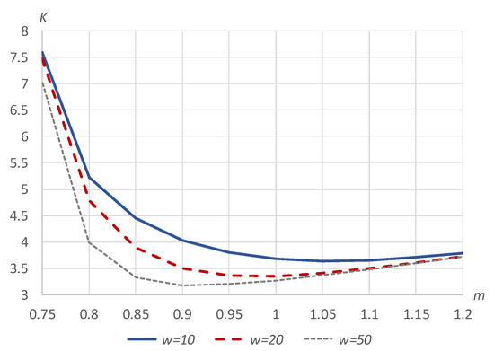
Figure 1. Values of the total cost $K\left(m\right)$ for various values of bound w.

9. Discussion

In this paper, we apply a new approach [22] for studying multi-server retrial queue with hyper-exponential service time. Analysis of the model is made under asymptotic condition of long delay in the orbit. Using asymptotic analysis technique [18,19], we obtain parameters of diffusion process Equation (45) which is used to build approximations for stationary probability distributions of the number of customers in the orbit Equation (51) and the number of busy servers Equations (52)–(54).

We use numerical experiments and simulations for estimation of the approximations accuracy. Using Kolmogorov distance $\Delta$ Equation (55) as an error of approximation and criteria of approximation applicability in the form $\Delta \le 0.05$, we obtain applicability areas of proposed approximations. As it shown, these areas are wide enough. At least in the most of cases, they are wider than applicability areas of approximations obtained using basic asymptotic analysis technique as it was made in [18,19,20,21].

We suppose to use asymptotic diffusion method and obtained results in future works that will be devoted as to analysis of retrial queues with other configurations both to study of multi-server retrial queue with arbitrary distributed service time. Using hyper-exponential distribution as an approximation for distributions of other types may be the first step in this direction. Further studies may involve supplementary variables technique or using Markov chains based on departure epochs.

We thank the reviewers of this paper whose comments allow us improve the work.

References

- Aguir, S.; Karaesmen, F.; Askin, O.Z.; Chauvet, F. The impact of retrials on call center performance. OR Spektrum 2004, 26, 353–376. [Google Scholar] [CrossRef]
- Stolletz, R. Performance Analysis and Optimization of Inbound Call Centers; Springer: Berlin/Heidelberg, Germany, 2003. [Google Scholar]
- Avrachenkov, K.; Yechiali, U. Retrial networks with finite buffers and their application to internet data traffic. Probab. Eng. Inf. Sci. 2008, 22, 519–536. [Google Scholar] [CrossRef]
- Roszik, J.; Sztrik, J.; Kim, C.S. Retrial queues in the performance modelling of cellular mobile networks using MOSEL. Int. J. Simul. 2005, 6, 38–47. [Google Scholar]
- Artalejo, J.R.; Lopez-Herrero, M.J. Cellular mobile networks with repeated calls operating in random environment. Comput. Oper. Res. 2010, 37, 1158–1166. [Google Scholar] [CrossRef]
- Ke, X.; Shi, L.; Guo, W.; Chen, D. Multi-Dimensional Traffic Congestion Detection Based on Fusion of Visual Features and Convolutional Neural Network. IEEE Trans. Intell. Trans. Syst. 2019, 20, 2157–2170. [Google Scholar] [CrossRef]
- Nazarov, A.A.; Moiseev, A.N. Distributed System of Processing of Data of Physical Experiments. Rus. Phys. J. 2014, 57, 984–990. [Google Scholar] [CrossRef]
- Phung-Duc, T. Retrial Queueing Models: A Survey on Theory and Applications. arXiv 2019, arXiv:1906.09560v1. [Google Scholar]
- Falin, G.I.; Templeton, J.G.C. Retrial Queues; Chapman & Hall: London, UK, 1997. [Google Scholar]
- Falin, G.I. A survey of retrial queues. Queueing Syst. 1990, 7, 127–168. [Google Scholar] [CrossRef]
- Artalejo, J.R.; Gomez-Corral, A. Retrial Queueing Systems: A Computational Approach; Springer: Berlin/Heidelberg, Germany, 2008. [Google Scholar]
- Shekhar, C.; Raina, A.A.; Kumar, A. A brief review on retrial queue: Progress in 2010–2015. Int. J. Appl. Sci. Eng. Res. 2016, 5, 324–336. [Google Scholar]
- Kim, C.; Mushko, V.; Dudin, A. Computation of the steady state distribution for multi-server retrial queues with phase type service process. Ann. Oper. Res. 2012, 201, 307–323. [Google Scholar] [CrossRef]
- Phung-Duc, T.; Masuyama, H.; Kasahara, S.; Takahashi, Y. A matrix continued fraction approach to multiserver retrial queues. Ann. Oper. Res. 2013, 203, 161–183. [Google Scholar] [CrossRef]
- Neuts, M.; Rao, B. Numerical investigation of a multiserver retrial mode. Queueing Syst. 2002, 7, 169–189. [Google Scholar] [CrossRef]
- Artalejo, J.; Pozo, M. Numerical calculation of the stationary distribution of the main multiserver retrial queue. Ann. Oper. Res. 2002, 116, 41–56. [Google Scholar] [CrossRef]
- Ridder, A. Fast simulation of retrial queues. In Proceedings of the 3rd Workshop on Rare Event Simulation and Related Combinatorial Optimization Problems, Pisa, Italy, 5–6 October 2000. [Google Scholar]
- Moiseeva, E.; Nazarov, A. Asymptotic analysis of RQ-systems M/M/1 on heavy load condition. In Proceedings of the IV International Conference Problems of Cybernetics and Informatics, Baku, Azerbaijan, 12–14 September 2012; pp. 164–166. [Google Scholar]
- Fedorova, E. Quasi-geometric and gamma approximation for retrial queueing systems. Commun. Comput. Inf. Sci. 2014, 487, 123–136. [Google Scholar]
- Nazarov, A.; Chernikova, Y. Gaussian approximations of probabilities distribution of states of the retrial queueing system with r-persistent exclusion of alternative customers. Commun. Comput. Inf. Sci. 2015, 564, 200–209. [Google Scholar]
- Lapatin, I.; Nazarov, A. Asymptotic Analysis of the Output Process in Retrial Queue with Markov-Modulated Poisson Input Under Low Rate of Retrials Condition. Commun. Comput. Inf. Sci. 2019, 1141, 315–324. [Google Scholar]
- Nazarov, A.; Phung-Duc, T.; Paul, S.; Lizura, O. Asymptotic-Diffusion Analysis for Retrial Queue with Batch Poisson Input and Multiple Types of Outgoing Calls. Lect. Notes Comput. Sci. 2019, 11965, 207–222. [Google Scholar]
- Moiseev, A.; Demin, A.; Dorofeev, V.; Sorokin, V. Discrete-event approach to simulation of queueing networks. Key Eng. Mater. 2016, 685, 939–942. [Google Scholar] [CrossRef]
- Mesheryakov, R.; Moiseev, A.; Demin, A.; Dorofeev, V.; Sorokin, V. Using parallel computing in queueing network simulation. Key Eng. Mater. 2016, 685, 943–947. [Google Scholar] [CrossRef]
© 2020 by the authors. Licensee MDPI, Basel, Switzerland. This article is an open access article distributed under the terms and conditions of the Creative Commons Attribution (CC BY) license (http://creativecommons.org/licenses/by/4.0/).