On the Connection between Spherical Laplace Transform and Non-Euclidean Fourier Analysis

Abstract

We prove that, if the coefficients of a Fourier–Legendre expansion satisfy a suitable Hausdorff-type condition, then the series converges to a function which admits a holomorphic extension to a cut-plane. Next, we introduce a Laplace-type transform (the so-called Spherical Laplace Transform) of the jump function across the cut. The main result of this paper is to establish the connection between the Spherical Laplace Transform and the Non-Euclidean Fourier Transform in the sense of Helgason. In this way, we find a connection between the unitary representation of $\mathrm{SO}\left(3\right)$ and the principal series of the unitary representation of $\mathrm{SU}(1,1)$.

1. Introduction

It is well known that the classical Fourier transform refers to the decomposition of a function belonging to an appropriate space into exponentials, which can be viewed as the irreducible unitary representations of the additive group of the real numbers. However, in the current most popular interpretation, particularly in connection with non-commutative groups, the phrase harmonic analysis has lost its original function-theoretic meaning and now it generally refers not to functions but to representations. It thus becomes natural to regard irreducible representations as the basic building blocks of the theory in place of exponential functions [1]. There are however examples in the theory of the semi-simple non-compact Lie groups where the classical setup prevails, in the sense that one can find a class of functions which play a role similar to that played by the exponentials on the real line. A typical example thereof is the group $\mathrm{SU}(1,1)$: hereafter, we shall work at the level of homogeneous spaces associated with this group and, accordingly, we shall study the spherical functions that can be constructed in these spaces.

Within this framework, a fundamental role is played by the Helgason construction of the so-called non-Euclidean Fourier analysis [2]. The working ambient is the symmetric space $\mathrm{SU}(1,1)/\mathrm{SO}\left(2\right)$, i.e., the non-Euclidean disk. By the use of the Poisson kernel, the analog of the plane waves are constructed in the case of the hyperbolic disk and, successively, an integral representation of the conical functions $P_{-\frac{1}{2}+\mathrm{i}\mu }(coshr)$ (i.e., the Legendre functions of the first kind with index $(-\frac{1}{2}+\mathrm{i}\mu )$, $\mu \in \mathbb{R}$) is derived in terms of these hyperbolic waves. It can thus be proved for these functions a product formula, which corresponds to the classical product formula of the exponentials. Finally, a Fourier transform on the non-Euclidean disk can be set up, which is exactly the tool analogous to the classical Fourier transform. In this connection, it is worth recalling that the conical functions can be associated with the principal series of the irreducible unitary representation of the group $\mathrm{SU}(1,1)$, which acts transitively on the hyperbolic disk.

Consider now an isotropic cone in ${\mathbb{R}}^3$. We focus on the two-sheeted hyperboloid interior to the cone. By stereographic projection, the upper sheet of the two-sheeted hyperboloid can be mapped into the interior of the unit disk. Since the connected component of the two-sheeted hyperboloid is the homogeneous space ${\mathrm{SO}}_0(1,2)/\mathrm{SO}\left(2\right)$, the non-Euclidean Fourier analysis coincides with the harmonic analysis on ${\mathrm{SO}}_0(1,2)/\mathrm{SO}\left(2\right)$. We can thus define and study the Fourier transform on the two-sheeted hyperboloid.

Harmonic analysis can be studied also on the one-sheeted hyperboloid, which is a pseudo-Riemannian symmetric space ${\mathrm{SO}}_0(1,2)/{\mathrm{SO}}_0(1,1)$. It is then possible to construct on this symmetric space spherical functions, which turn out to be the Legendre functions of the second kind. A peculiar feature of this space is that it can be equipped with the partial ordering associated with the light cone in ${\mathbb{R}}^3$: namely, $x⩾y\iff (x-y)$ belongs to the closed future cone of ${\mathbb{R}}^3$. The one-sheeted hyperboloid equipped with this ordering relation is a causal symmetric space [3]. Accordingly, we can introduce a Volterra algebra of kernels, i.e., kernels $K(x,y)$ whose support is contained in the set $\mathsf{\Gamma }\doteq \{(x,y)\in X_2\times X_2:x⩾y\}$, where $X_2$ is the one-sheteed hyperboloid. A kernel K is said to be invariant under $G\equiv {\mathrm{SO}}_0(1,2)$ if for any $g\in G$: $K(gx,gy)=K(x,y)$, $(x,y)\in \mathsf{\Gamma }$. An invariant Volterra kernel K can be identified with a function f on G through the equality: $K(g{e}_2,e_2)=f\left(g\right)$, where $g\in G$ and $e_2=(0,0,1)$ (see next Figure 1) is the point which features $h{e}_2=e_2$, with $h\in {\mathrm{SO}}_0(1,1)$ [4,5,6,7]. Successively, the spherical Laplace transform for this class of functions can be defined. This transform, as the ordinary Laplace transform, is holomorphic in a half-plane and, in the specific case of the spherical Laplace transform, this analyticity property follows from the analyticity property of the Legendre functions of the second kind $Q_{\lambda }(·)$, which are holomorphic in the half-plane ${\mathbb{C}}_{(-1)}^{(+)}\doteq \{\lambda \in \mathbb{C}:\mathrm{Re}\lambda >-1\}$. These latter functions are indeed the spherical functions on ordered symmetric spaces in the sense of Faraut et al. [7].

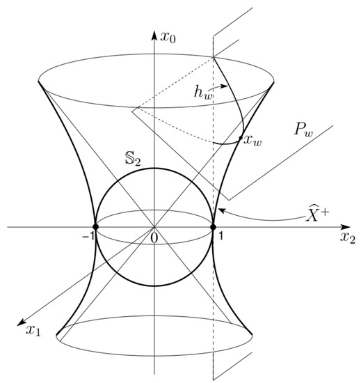
Figure 1. Horocyclic fibration of the one-sheteed hyperboloid $X_2^{+}$.

Another question closely related to this type of problems is the holomorphic extension associated with Fourier–Legendre expansions of the type: $\frac{1}{4\pi }{\sum }_{n=0}^{\infty }(2n+1)a_n{P}_n(cos\theta )$, where $P_n(·)$ denotes the Legendre polynomials. In this paper, we prove that, if the sequence ${\left\{{(n+1)}^2{a}_n\right\}}_{n=0}^{\infty }$ satisfies a suitable Hausdorff-type condition [8], then the function $f(cos\theta )$, to which the Fourier–Legendre series converges in the interval $(-1,1)$, admits a holomorphic extension to the complex $cos\theta$-plane cut along the semi-axis $[1,+\infty )$. The first result we prove is a basic feature of the holomorphic extension associated with Fourier–Legendre series: the dual analyticity property. To classes of functions which are holomorphic in the $cos\theta$-plane cut along $[1,+\infty )$, there correspond classes of functions, denoted $\tilde{a}\left(\lambda \right)$ ($\lambda \in \mathbb{C}$), which are expressed as a spherical Laplace transform, holomorphic in the half-plane $\mathrm{Re}\lambda >-\frac{1}{2}$, of Carlsonian-type (i.e., of suitable exponential growth; see next Theorem 1) and, therefore, unique interpolants of the coefficients $a_n$ of the Fourier-Legendre series, i.e., $\tilde{a}{\left(\lambda \right)|}_{\lambda =n}=a_n$ ($n=0,1,2,\dots$).

At this point, two strictly related problems emerge. On the one hand, the possibility of connecting, via analytic continuation, the completeness of the spherical functions for $\mathrm{SO}\left(3\right)$ to the completeness of the corresponding expansion of $\mathrm{SL}(2,\mathbb{R})$, which is the group acting transitively on the upper half-plane, where the model of the non-Euclidean geometry can be realized, while, on the other hand, continuing the unitary representations of $\mathrm{SO}\left(3\right)$ to give the unitary representations of $\mathrm{SL}(2,\mathbb{R})$. The first problem has been initially tackled by Stein and Wainger [9], while, for what concerns the second one, the reader is referred to the work of R. Hermann [10]. However, both of these problems require linking the spherical Laplace transform to the non-Euclidean Fourier analysis. When we consider the ordinary Laplace transform of a function $f\in L^1(0,+\infty )\cap L^2(0,+\infty )$,

$$\tilde{f}\left(\lambda \right)={\int }_0^{+\infty }{e}^{-\lambda v}f\left(v\right)\mathrm{d}v(\lambda \in \mathbb{C},\mathrm{Re}\lambda >0),$$

we obtain for $\lambda =\mathrm{i}\mu$ ($\mu \in \mathbb{R}$):

$$\tilde{f}\left(\mathrm{i}\mu \right)={\int }_{-\infty }^{+\infty }{e}^{-\mathrm{i}\mu v}f\left(v\right)\mathrm{d}v(\mu \in \mathbb{R}),$$

which is precisely the Fourier transform of $f\left(v\right)$, it being well-defined in view of the assumption $f\in L^1(0,+\infty )$. Since $f\in L^1(0,+\infty )\cap L^2(0,+\infty )$, the Fourier transform can be inverted to recover $f\left(v\right)$ in terms of $\tilde{f}\left(\mathrm{i}\mu \right)$ through the inverse Fourier transform, which converges to $f\left(v\right)$ as a limit in the mean order two. Correspondingly, we pass from the non-unitary representation $e^{-\lambda v}$ ($\lambda \in \mathbb{C},\mathrm{Re}\lambda >0,\mu \equiv \mathrm{Im}\lambda \in \mathbb{R}$) to the unitary irreducible representation $e^{-\mathrm{i}\mu v}$ ($\mu ,v\in \mathbb{R}$) that we mentioned at the beginning of the Introduction. This connection can be extended. One of our results consists indeed of proving that the spherical Laplace transform reduces to the non-Euclidean Fourier transform at $\mathrm{Re}\lambda =-\frac{1}{2}$, which is precisely the value corresponding to the principal series of the unitary representations of the group $\mathrm{SU}(1,1)$, which acts transitively on the hyperbolic disk. This result has been obtained by establishing a bridge between the harmonic analysis on the one-sheeted hyperboloid and the harmonic analysis on the two-sheeted hyperboloid.

The harmonic analysis in causal symmetric spaces has been a subject of growing interest in the last three decades, and the research on these topics has flowed in various directions. Some papers have been devoted to the proof of the Paley–Wiener theorem for spherical Laplace transform [11,12] and others have treated the inversion problem extended up to the so-called $\Theta$-transform [13]. In [14], Bertram has studied the compact symmetric space and its non-compact dual, both realized as real forms of their common complexification; this analysis has been performed by exploring the Ramanujan garden and by the use of the so-called Master Theorem. Working in a different direction, Gindinkin and Krötz [15] have studied the complex crown of Riemannian symmetric spaces and non-compactly causal symmetric spaces. This allowed them to prove the conjecture that every non-compactly causal symmetric space occurs as a component of a distinguished boundary of some complex crown [15]. Finally, it is worth recalling that the question of relating the harmonic analysis of different real forms of a complex symmetric space has been studied also in the context of scattering theory and resonances [16,17,18,19,20].

The paper is organized as follows. In Section 2, we study the holomorphic extension associated with the Fourier–Legendre expansion by means of the spherical Laplace transform. We are thus led to develop the harmonic analysis on the complex one-sheeted hyperboloid $X_2^{\left(c\right)}$, which contains as submanifolds either the Euclidean sphere $(\mathrm{i}\mathbb{R}\times {\mathbb{R}}^2)\cap X_2^{\left(c\right)}$ on which the Fourier–Legendre expansion can be developed, and the real one-sheeted hyperboloid, which contains the support of the cut. In Section 3, we analyze the relationship between the spherical Laplace transform and the non-Euclidean Fourier transform. For this purpose, we consider a real two-sheeted hyperboloid, and, in this geometrical setting, we can recover the non-Euclidean Fourier transform in the sense of Helgason. Finally, in Section 4, some conclusions will be drawn.

2. Holomorphic Extension Associated with the Fourier–Legendre Expansion and the Spherical Laplace Transform

2.1. The Complex One-Sheeted Hyperboloid

In the space ${\mathbb{C}}^3$ of the variable $z=(z_0,z_1,z_2)$, we consider the complex quadric $X_2^{\left(c\right)}$ with equation

$$-z_0^2+z_1^2+z_2^2=1,$$

which is a one-sheeted complex hyperboloid. Next, we introduce two systems of coordinates: polar and horocyclic coordinates.

Polar Coordinates:

$$\begin{array}{cc}\hfill z_0& =-\mathrm{i}sin\theta cosh\phi ,\hfill \end{array}$$

(1a)

$$\begin{array}{cc}\hfill z_1& =-\mathrm{i}sin\theta sinh\phi ,(\theta ,\phi \in \mathbb{C}),\hfill \end{array}$$

(1b)

$$\begin{array}{cc}\hfill z_2& =cos\theta .\hfill \end{array}$$

(1c)

If $\theta =u$ ($u\in \mathbb{R}$) and $\phi =\mathrm{i}\psi$ ($\psi \in \mathbb{R}$), (1) reads

$$\begin{array}{cc}\hfill x_0& =-\mathrm{i}sinucos\psi ,\hfill \end{array}$$

(2a)

$$\begin{array}{cc}\hfill x_1& =sinusin\psi ,(u,\psi \in \mathbb{R}),\hfill \end{array}$$

(2b)

$$\begin{array}{cc}\hfill x_2& =cosu.\hfill \end{array}$$

(2c)

It can be easily verified that: $-x_0^2+x_1^2+x_2^2={sin}^{2}u+{cos}^{2}u=1$ that is, one obtains as a real submanifold of the complex one-sheeted hyperboloid $X_2^{\left(c\right)}$ the Euclidean sphere ${\mathbb{S}}_2=(\mathrm{i}\mathbb{R}\times {\mathbb{R}}^2)\cap X_2^{\left(c\right)}$ ($\mathrm{i}\mathbb{R}$ referring to the coordinate $z_0$ of z).

Similarly, if $\theta =\mathrm{i}v$ ($v\in \mathbb{R}$) and $\phi =\psi$ ($\psi \in \mathbb{R}$), (1) becomes

$$\begin{array}{cc}\hfill x_0& =sinhvcosh\psi ,\hfill \end{array}$$

(3a)

$$\begin{array}{cc}\hfill x_1& =sinhvsinh\psi ,(v,\psi \in \mathbb{R}),\hfill \end{array}$$

(3b)

$$\begin{array}{cc}\hfill x_2& =coshv.\hfill \end{array}$$

(3c)

In this case, it is easily verified that: $-x_0^2+x_1^2+x_2^2={cosh}^{2}v-{sinh}^{2}v=1$. Equation (3) describes only the subset $X_2^{+}\doteq \{x\in X_2:x_2⩾1\}$ of the real one-sheeted hyperboloid $X_2$, which is precisely what we need for the current analysis. Finally, let ${\widehat{X}}^{+}$ denote the (real) meridian lying in the plane $x_1=0$ with equation: $x_0^2-x_2^2=-1$.

Horocyclic Coordinates:

We now introduce another system of coordinates $(\tau ,\zeta )$ as follows:

$$\begin{array}{cc}\hfill z_0& =-\mathrm{i}sin\tau +\frac{1}{2}{\zeta }^2{e}^{-\mathrm{i}\tau },\hfill \end{array}$$

(4a)

$$\begin{array}{cc}\hfill z_1& =\zeta e^{-\mathrm{i}u},(\tau ,\zeta \in \mathbb{C}),\hfill \end{array}$$

(4b)

$$\begin{array}{cc}\hfill z_2& =cos\tau -\frac{1}{2}{\zeta }^2{e}^{-\mathrm{i}\tau }.\hfill \end{array}$$

(4c)

For $\tau =\mathrm{i}w$ ($w\in \mathbb{R}$) and $\zeta \in \mathbb{R}$, Equation (4) reads

$$\begin{array}{cc}\hfill x_0& =sinhw+\frac{1}{2}{\zeta }^2{e}^w,\hfill \end{array}$$

(5a)

$$\begin{array}{cc}\hfill x_1& =\zeta e^w,(w,\zeta \in \mathbb{R}),\hfill \end{array}$$

(5b)

$$\begin{array}{cc}\hfill x_2& =coshw-\frac{1}{2}{\zeta }^2{e}^w.\hfill \end{array}$$

(5c)

Then, we consider the intersection points $x_w$ of ${\widehat{X}}^{+}$ with the family of planes $P_w:x_0+x_2=e^w$ ($w\in \mathbb{R}$) (see Equation (5)), i.e., the points $x_w=(sinhw,0,coshw)$. The sections of $X_2$ by these planes are the (real) parabolae ${\mathsf{\Pi }}_w^{+}$ (except in the case $x_0+x_2=0$). When $\zeta =0$ in (5), we obtain the point $x_w$, which is the apex of the corresponding parabola ${\mathsf{\Pi }}_w^{+}$ (see Figure 1).

This geometrical construction can now be extended to the complex one-sheeted hyperboloid $X_2^{\left(c\right)}$. We consider the (complex) hyperbola ${\widehat{X}}^{\left(c\right)}$ lying in the plane $z_1=0$, whose equation is: $z_0^2-z_2^2=-1$ (see Equation (4)), and its intersections with the family of planes $P_{\tau }$ with equation $z_0+z_2=e^{-\mathrm{i}\tau }$ ($\tau \in \dot{\mathbb{C}}\doteq \mathbb{C}/2\pi \mathbb{Z}$). Each plane $P_{\tau }$ intersects the hyperbola ${\widehat{X}}^{\left(c\right)}$ at the (unique) point $z_{\tau }=(z_0=-\mathrm{i}sin\tau ,z_1=0,z_2=cos\tau )$, thus defining a bijection from the set of planes $\mathcal{P}\doteq \{P_{\tau }:\tau \in \dot{\mathbb{C}}\}$ onto ${\widehat{X}}^{\left(c\right)}=\{z_{\tau }:\tau \in \dot{\mathbb{C}}\}$. For each $\tau \in \dot{\mathbb{C}}$, the manifold $P_{\tau }\cap X_2^{\left(c\right)}$ is a complex parabola ${\mathsf{\Pi }}_{\tau }$, which we call a complex horocycle. The set of horocycles $\{{\mathsf{\Pi }}_{\tau }:\tau \in \dot{\mathbb{C}}\}$ defines a fibration with basis ${\widehat{X}}^{\left(c\right)}$ on the dense domain ${X_2^{\prime }}^{\left(c\right)}\doteq \{z\in X_2^{\left(c\right)}:z_0+z_2\ne 0\}$ of $X_2^{\left(c\right)}$. We can therefore associate with this fibration the parametric representation of ${X_2^{\prime }}^{\left(c\right)}$ given by Equation (4), $(\tau ,\zeta )$ being the horocyclic coordinates of the point $z\in {X_2^{\prime }}^{\left(c\right)}$.

2.2. The Radon Transform

We now define a Radon-type transformation in $X_2$, where the horocycles defined above play the same role as the planes do in the ordinary Radon transformation. We introduce the following integral:

$${\int }_{h_w}\underline{F}\left(coshw-\frac{1}{2}{\zeta }^2{e}^w\right)\mathrm{d}\zeta =\widehat{F}\left(w\right),$$

(6)

where $h_w$ is the oriented segment of horocycle, which is represented by the arc of parabola whose apex is obtained by setting $\zeta =0$ in (5) (i.e., its coordinates are: $x_0=sinhw$, $x_1=0$, $x_2=coshw$; $w\in \mathbb{R}$), and whose endpoints lie on the plane $x_2=1$. The function $\underline{F}$ is assumed to satisfy the regularity conditions that make integral (6) convergent.

Remark 1.

Legendre expansions, which will be our concern later, involve functions depending only on $cosu=x_2$ (see (2c)). This is why, in the integral (6), we limit ourselves to consider functions only of the form $\underline{F}=\underline{F}(coshw-\frac{1}{2}{\zeta }^2{e}^w)$ (see (5c)).

Since the integrand in (6) is an even function of $\zeta$, the integration domain can be restricted to the part $h_w^{+}$ of $h_w$ with $x_1⩾0$, which can be parametrized as follows (see (5)):

$$h_w^{+}=\{x\in {\mathsf{\Pi }}_w^{+};x=x(\zeta ,w);\zeta \left(\delta \right)={\left[2e^{-w}(1-\delta )(coshw-1)\right]}^{\frac{1}{2}};0⩽\delta ⩽1\}(w\in \mathbb{R}),$$

(7)

positively oriented from the apex to the endpoint lying on $x_2=1$. For $\delta =1$, we have $\zeta =0$, which yields the apex of the parabola representing the horocycle; for $\delta =0$, we have $\zeta ={\left[2e^{-w}(coshw-1)\right]}^{1/2}$, which gives the intersection of the horocycle with the plane $x_2=1$.

We may now introduce another parametrization of the segment of horocycle $h_w^{+}$, which is obtained by setting $x_2=coshv$ (see (3c)):

$$h_w^{+}=\{x\in {\mathsf{\Pi }}_w^{+};x=x(\zeta ,w);\zeta \left(v\right)={\left[2e^{-w}(coshw-coshv)\right]}^{\frac{1}{2}};0⩽v⩽w\}(w\in \mathbb{R}).$$

(8)

Indeed, we have $\zeta =0$ for $v=w$ (the apex of the parabola) and $\zeta ={\left[2e^{-w}(coshw-1)\right]}^{1/2}$ for $v=0$ (endpoint of the parabola: $x_2=coshv=1$). Since $\mathrm{d}\zeta /\mathrm{d}v=-e^{-w/2}sinhv{\left[2(coshw-coshv)\right]}^{-1/2}$, integral (6) takes the form:

$$\widehat{F}\left(w\right)=2e^{-w/2}{\int }_0^w\underline{F}(coshv)\frac{sinhv}{{\left[2(coshw-coshv)\right]}^{\frac{1}{2}}}\mathrm{d}v\doteq e^{-w/2}\left(\mathcal{A}F\right)\left(w\right)(w\in \mathbb{R}),$$

(9)

where $\left(\mathcal{A}F\right)\left(w\right)$ is an Abel-type integral.

The fibration realized by the horocycles ${\mathsf{\Pi }}_w^{+}$ can now be extended to the complex domain by using the complex horocycles ${\mathsf{\Pi }}_{\tau }$ ($\tau =t+\mathrm{i}w;t,w\in \mathbb{R}$), whose intersection with the (complex) meridian hyperbola ${\widehat{X}}^{\left(c\right)}$ is the point $z_{\tau }=(-\mathrm{i}sin\tau ,0,cos\tau )$. Accordingly, we introduce the following integral:

$$2{\int }_{h_{\tau }^{+}}\underline{f}\left(cos\tau -\frac{1}{2}{\zeta }^2{e}^{-\mathrm{i}\tau }\right)\mathrm{d}\zeta =\widehat{f}\left(\tau \right),$$

(10)

$h_{\tau }^{+}$ being the (oriented) arc of the complex horocycle defined by (see (4) and (7)):

$$h_{\tau }^{+}=\{z\in {\mathsf{\Pi }}_{\tau };z=z(\zeta ,\tau );\zeta \left(\delta \right)={\left[2e^{\mathrm{i}\tau }(1-\delta )(cos\tau -1)\right]}^{\frac{1}{2}};0⩽\delta ⩽1\}(\tau \in \mathbb{C}).$$

For $\delta =1$, we have $\zeta =0$, i.e., the point $z_{\tau }$ belonging to ${\widehat{X}}^{\left(c\right)}$, while for $\delta =0$ we have $\zeta ={\left[2e^{\mathrm{i}\tau }(cos\tau -1)\right]}^{1/2}$, which is the intersection of $h_{\tau }^{+}$ with the plane $z_2=1$. Similarly to what done before, we may now introduce the following parametrization of $h_{\tau }^{+}$, obtained by setting $z_2=cos\theta$ ($\theta \in \mathbb{C},\theta =u+\mathrm{i}v$; see (1) and (8)):

$$h_{\tau }^{+}=\{z\in {\mathsf{\Pi }}_{\tau };z=z(\zeta ,\tau );\zeta \left(\theta \right)={\left[2e^{\mathrm{i}\tau }(cos\tau -cos\theta )\right]}^{\frac{1}{2}};\theta \in {\gamma }_{\tau }\}(\tau \in \mathbb{C}),$$

where ${\gamma }_{\tau }$ denotes the ray in the $\theta$-plane oriented from 0 to $\tau$:

$${\gamma }_{\tau }=\{\theta =\theta \left(\delta \right);cos\theta \left(\delta \right)-1=\delta (cos\tau -1);0⩽\delta ⩽1\}(\tau \in \mathbb{C}).$$

Now, since $\mathrm{d}\zeta /\mathrm{d}\theta =e^{\mathrm{i}\tau /2}{\left[2(cos\tau -cos\theta )\right]}^{-1/2}sin\theta$, integral (10) can be rewritten in the form:

$$\widehat{f}\left(\tau \right)=-2e^{\mathrm{i}\tau /2}{\int }_{{\gamma }_{\tau }}f\left(\theta \right)\frac{sin\theta }{{\left[2(cos\tau -cos\theta )\right]}^{\frac{1}{2}}}\mathrm{d}\theta ,$$

(11)

where $f\left(\theta \right)\equiv \underline{f}(cos\theta )$. The relevant branch of the function ${\left[2(cos\tau -cos\theta )\right]}^{-1/2}$ is specified by the condition that, for $\tau =\mathrm{i}w$ and $\theta =\mathrm{i}v$ (with $w>v$), it takes the value ${\left[2(coshw-coshv)\right]}^{-1/2}⩾0$. Putting in (11) $\tau =\mathrm{i}w$, $\theta =\mathrm{i}v$, we re-obtain precisely the r.h.s. of formula (9), once $\underline{f}$ is identified with $\underline{F}$.

Restricting formula (11) to the set of real values for the variables $\tau$ and $\theta$, namely, $\tau =t$ and $\theta =u$ ($t,u\in \mathbb{R}$), from (11), we obtain

$$\widehat{f}\left(t\right)=-2e^{\mathrm{i}t/2}{\int }_0^{t}f\left(u\right)\frac{sinu}{{\left[2(cost-cosu)\right]}^{\frac{1}{2}}}\mathrm{d}u.$$

(12)

Accounting for the relevant branch of the factor ${\left[2(cos\tau -cos\theta )\right]}^{-1/2}$ in (11), formula (12) can be written in the following more precise form (involving a positive bracket):

$$\widehat{f}\left(t\right)=-2\mathrm{i}\epsilon \left(t\right)e^{\mathrm{i}t/2}{\int }_0^{t}f\left(u\right)\frac{sinu}{{\left[2(cosu-cost)\right]}^{\frac{1}{2}}}\mathrm{d}u,$$

(13)

where $\epsilon \left(t\right)$ denotes the sign function.

2.3. Holomorphic Extension Associated with Trigonometric Series

2.3.1. Fourier–Legendre Expansions as Trigonometric Series

Consider the following Legendre series

$$\frac{1}{4\pi }\sum _{n=0}^{\infty }(2n+1)a_n{P}_n(cosu),$$

(14)

where $P_n(·)$ denotes the Legendre polynomials, which satisfy the following integral representation:

$$P_n(cosu)=\frac{1}{\pi }{\int }_0^{\pi }{(cosu+\mathrm{i}sinucos\eta )}^n\mathrm{d}\eta .$$

Suppose that expansion (14) converges to a function $\underline{f}(cosu)$ absolutely integrable in the interval $u\in [0,\pi ]$. Then, the Legendre coefficients $a_n$ can be written as

$$a_n=2\pi {\int }_0^{\pi }\underline{f}(cosu)P_n(cosu)sinu\mathrm{d}u.$$

In Ref. [21], we proved the following proposition.

Proposition 1.

The Legendre coefficients ${\left\{a_n\right\}}_{n=0}^{\infty }$ coincide with the Fourier coefficients of the following form:

$$a_n={\int }_{-\pi }^{\pi }\widehat{f}\left(t\right)e^{\mathrm{i}nt}\mathrm{d}t(n=0,1,2,\dots ),$$

(15)

where

$$\widehat{f}\left(t\right)=-2\mathrm{i}\epsilon \left(t\right)e^{\mathrm{i}t/2}{\int }_0^{t}f\left(u\right)\frac{sinu}{{\left[2(cosu-cost)\right]}^{\frac{1}{2}}}\mathrm{d}u,$$

(16)

with $f\left(u\right)\equiv \underline{f}(cosu)$, and $\epsilon \left(t\right)$ being the sign function.

Proof. 

See Proposition 3.1 of Ref. [21]. □

Note that (16) coincides with (13). From (16), it is easy to verify that

$$\widehat{f}\left(t\right)=-e^{\mathrm{i}t}\widehat{f}(-t),$$

(17)

which, through (15), yields the following symmetry relation for the Legendre coefficients:

$$a_n=-a_{-n-1}(n\in \mathbb{Z}).$$

(18)

Now, we can introduce the following trigonometric series, assuming (18) to hold:

$$\begin{array}{c}\frac{1}{2\pi }\sum _{n=-\infty }^{+\infty }{a}_n{e}^{-\mathrm{i}nt}=\frac{1}{2\pi }\left[\sum _{n=0}^{+\infty }{a}_n{e}^{-\mathrm{i}nt}-e^{\mathrm{i}t}\sum _{n=0}^{+\infty }{a}_n{e}^{\mathrm{i}nt}\right]\hfill \\ =\frac{1}{2\pi }{e}^{\mathrm{i}(t-\pi )/2}\sum _{n=-\infty }^{+\infty }{(-1)}^n{a}_{n}cos\left[\left(n+\frac{1}{2}\right)(t-\pi )\right]=\frac{1}{2\pi }{e}^{\mathrm{i}(t-\pi )/2}\sum _{n=-\infty }^{+\infty }{a}_{n}sin\left[\left(n+\frac{1}{2}\right)t\right],\hfill \end{array}$$

(19)

and study the associated holomorphic extension.

2.3.2. Holomorphic Extension Associated with Trigonometric Series

Consider a sequence ${\left\{f_n\right\}}_{n=0}^{\infty }$ of (real) numbers, and denote by $∆$ the difference operator:

$$∆f_n=f_{n+1}-f_n.$$

We have:

$${∆}^k{f}_n=\underset{k-\mathrm{times}}{\underbrace{∆\times ∆\times \cdots ∆}}{f}_n=\sum _{m=0}^k{(-1)}^m\left(\genfrac{}{}{0pt}{}{k}{m}\right)f_{n+k-m}$$

(for any integer $k⩾0$); ${∆}^0$ is the identity operator, by definition. Suppose that there exists a positive constant M such that

$${(n+1)}^{(1+\epsilon )}\sum _{i=0}^n{\left(\genfrac{}{}{0pt}{}{n}{i}\right)}^{(2+\epsilon )}{\left|{∆}^i{f}_{(n-i)}\right|}^{(2+\epsilon )}<M(n=0,1,2,\dots ;\epsilon >0).$$

(20)

We shall refer to (20) as the Hausdorff condition for its relevance in the solution of the Hausdorff moment problem [8]. The tool we use to guarantee uniqueness of the interpolation of a sequence of numbers ${\left\{f_n\right\}}_{n=0}^{\infty }$ is Carlson’s theorem [22]. Essentially, it gives growth conditions under which a function is uniquely determined by its values on non-negative integers. Let us recall that an entire function $f\left(z\right)$ is of exponential type $\tau <\infty$ if

$$\underset{r\to \infty }{lim\; sup}\frac{M_f\left(r\right))}{r}=\tau ,$$

(21)

where $M_f\left(r\right)$ denotes the maximum modulus of $f\left(z\right)$ for $\left|z\right|=r$. The rate of growth of entire functions can be specified along different directions by the Phragmén-Lindelöf indicator function,

$$h_f\left(\theta \right)=\underset{r\to \infty }{lim\; sup}\frac{log\left|f\left(r{e}^{\mathrm{i}\theta }\right)\right|}{r}.$$

(22)

Note that the preceding definitions can be extended to functions which are not entire, but regular (that is, analytic and single-valued) in a sector with vertex at the origin [22].

Theorem 1

(Carlson’s theorem (Section 9.2, p. 153, [22])). Let $f\left(z\right)$ be regular in the half-plane $\mathrm{Re}z⩾0$ and

(i) 

$f\left(z\right)$ is of exponential type $\tau <\infty$,

(ii) 

$h_f(\pi /2)+h_f(-\pi /2)<2\pi$,

(iii) 

$f\left(n\right)=0$ for $n=0,1,2,\dots$,

then $f\left(z\right)$ vanishes identically.

Among the functions of exponential type, condition (ii) requires $f\left(z\right)$ to be of exponential type less than $\pi$ on the imaginary axis that is: $f\left(\mathrm{i}y\right)=O\left(1\right)exp\left(c\right|y\left|\right)$ for some $c<\pi$. We shall refer to conditions (i) and (ii) as Carlson’s bound. Moreover, an analytic function which interpolates a sequence of numbers ${\left\{f_n\right\}}_{n=0}^{\infty }$ and satisfy conditions (i) and (ii) above will be called a Carlsonian interpolant, in view of the fact that the uniqueness of the interpolation is guaranteed by Carlson’s theorem.

Proposition 2.

Suppose that the set of numbers ${\left\{f_n\right\}}_{n=0}^{\infty }$, with $f_n\doteq {(n+1)}^2{a}_n$ ($a_n$ being the Fourier–Legendre coefficients of the series (14)), satisfies condition (20). Then:

(i) 

There exists a unique Carlsonian interpolant $\tilde{a}\left(\lambda \right)$ ($\lambda \in \mathbb{C},\mathrm{Re}\lambda ⩾-\frac{1}{2}$) of the coefficients ${\left\{a_n\right\}}_{n=0}^{\infty }$, which is holomorphic in the half-plane $\mathrm{Re}\lambda >-\frac{1}{2}$. Moreover, $\tilde{a}\left(\lambda \right)$ belongs to the Hardy space $H^2\left({\mathbb{C}}_{-1/2}^{(+)}\right)$.

(ii) 

${\lambda }^2\tilde{a}\left(\lambda \right)\in L^2(-\infty ,+\infty )$ for any fixed value of $\mathrm{Re}\lambda ⩾-\frac{1}{2}$.

(iii) 

${\lambda }^2\tilde{a}\left(\lambda \right)$ tends uniformly to zero as $\lambda \to \infty$ inside any fixed half-plane $\mathrm{Re}\lambda ⩾\delta >-\frac{1}{2}$.

(iv) 

$\lambda \tilde{a}\left(\lambda \right)\in L^1(-\infty ,+\infty )$ for any fixed value of $\mathrm{Re}\lambda ⩾-\frac{1}{2}$.

(v) 

$\tilde{a}(-\frac{1}{2}+\mathrm{i}\mu )$ ($\mu \in \mathbb{R}$) is a continuous function which tends to zero as $\mu \to \pm \infty$.

(vi) 

${sup}_{\stackrel{\sigma >-1/2}{\mu \in \mathbb{R}}}\left|\tilde{a}(\sigma +\mathrm{i}\mu )\right|=\left|\tilde{a}\left(-\frac{1}{2}+\mathrm{i}\mu \right)\right|$;

Proof. 

(i) Since the sequence ${\left\{f_n\right\}}_{n=0}^{\infty }$ satisfies condition (20), the numbers $f_n$ are moments of a suitable function, that is, the following representation holds [8]:

$$f_n={\int }_0^1{x}^n\phi \left(x\right)\mathrm{d}x(n=0,1,2,\dots ),$$

(23)

where $\phi \in L^{(2+\epsilon )}(0,1)$. Let $x=e^{-s}$ in formula (23):

$$f_n={\int }_0^{+\infty }{e}^{-(n+\frac{1}{2})s}{e}^{-s/2}\phi \left(e^{-s}\right)\mathrm{d}s(n=0,1,2,\dots ).$$

Then, the numbers ${\left\{f_n\right\}}_{n=0}^{\infty }$ can be formally regarded as the restriction to the (non-negative) integers of the following Laplace transform:

$$\tilde{f}\left(\lambda \right)={\int }_0^{+\infty }{e}^{-(\lambda +\frac{1}{2})s}{e}^{-s/2}\phi \left(e^{-s}\right)\mathrm{d}s\left(\mathrm{Re}\lambda >-\frac{1}{2}\right),$$

(24)

being $\tilde{f}{\left(\lambda \right)|}_{\lambda =n}=f_n$. We see that $e^{-s/2}\phi \left(e^{-s}\right)\in L^2(0,+\infty )$: in fact, ${\int }_0^{+\infty }|e^{-s/2}\phi \left(e^{-s}\right){|}^2\mathrm{d}s={\int }_0^1{\left|\phi \left(x\right)\right|}^2\mathrm{d}x<\infty$, since $\phi \in L^{(2+\epsilon )}(0,1)$ and, a fortiori, $\phi \left(x\right)\in L^2(0,1)$. Then, by the Paley–Wiener theorem [23], we have $\tilde{f}\left(\lambda \right)\in H^2\left({\mathbb{C}}_{-1/2}^{(+)}\right)$, which is the Hardy space whose norm is: $\parallel \tilde{f}{\parallel }_2\doteq {sup}_{\sigma >-1/2}({\int }_{-\infty }^{+\infty }|\tilde{f}(\sigma +\mathrm{i}\mu ){{|}^2\mathrm{d}\mu )}^{1/2}$, and ${\mathbb{C}}_{-1/2}^{(+)}\doteq \{\lambda \in \mathbb{C},\lambda =\sigma +\mathrm{i}\mu ;\sigma >-\frac{1}{2},\mu \in \mathbb{R}\}$. Hence, use can be made of Carlson’s theorem, which guarantees that $\tilde{f}\left(\lambda \right)$ is the unique Carlsonian interpolant of the sequence ${\left\{f_n\right\}}_{n=0}^{\infty }$. Let $\tilde{a}\left(\lambda \right)\doteq \tilde{f}\left(\lambda \right)/{(\lambda +1)}^2$. $\tilde{a}\left(\lambda \right)$ is a function holomorphic for $\mathrm{Re}\lambda >-\frac{1}{2}$, which satisfies Carlson’s bound since $\tilde{f}\left(\lambda \right)$ does. Then, $\tilde{a}\left(\lambda \right)$ is the unique Carlsonian interpolant of the set of Fourier–Legendre coefficients ${\left\{a_n\right\}}_{n=0}^{\infty }$ since $\tilde{a}{\left(\lambda \right)|}_{\lambda =n}={\left.\frac{\tilde{f}\left(\lambda \right)}{{(\lambda +1)}^2}\right|}_{\lambda =n}=\frac{f_n}{{(n+1)}^2}=a_n$. Finally, it is readily shown that $\tilde{a}\left(\lambda \right)\in H^2\left({\mathbb{C}}_{-1/2}^{(+)}\right)$:

$${∥\tilde{a}∥}_2^2=\underset{\sigma >-\frac{1}{2}}{sup}{\int }_{-\infty }^{+\infty }{\left|\frac{\tilde{f}(\sigma +\mathrm{i}\mu )}{{(\sigma +1+\mathrm{i}\mu )}^2}\right|}^2\mathrm{d}\mu ⩽16\underset{\sigma >-\frac{1}{2}}{sup}{\int }_{-\infty }^{+\infty }{\left|\tilde{f}(\sigma +\mathrm{i}\mu )\right|}^2\mathrm{d}\mu <\infty ,$$

(25)

and statement (i) is then proved. Regarding point (ii), since $\tilde{f}\left(\lambda \right)\in H^2\left({\mathbb{C}}_{-1/2}^{(+)}\right)$, then $\tilde{f}(\sigma +\mathrm{i}\mu )\in L^2(-\infty ,+\infty )$ for any fixed value of $\sigma ⩾-\frac{1}{2}$. Regarding point (iii), since $\tilde{f}\left(\lambda \right)\in H^2\left({\mathbb{C}}_{-1/2}^{(+)}\right)$, then $\tilde{f}\left(\lambda \right)$ tends to zero as $\lambda \to \infty$ inside any fixed half-plane $\mathrm{Re}\lambda ⩾\delta >-\frac{1}{2}$ [23]. By Schwarz’s inequality, we have for $\sigma ⩾-\frac{1}{2}$,

$${\int }_{-\infty }^{+\infty }\left|(\sigma +\mathrm{i}\mu )\tilde{a}(\sigma +\mathrm{i}\mu )\right|\mathrm{d}\mu ⩽{\left({\int }_{-\infty }^{+\infty }{\left|\frac{\sigma +\mathrm{i}\mu }{{(\sigma +1+\mathrm{i}\mu )}^2}\right|}^2\mathrm{d}\mu \right)}^{\frac{1}{2}}{\left({\int }_{-\infty }^{+\infty }{\left|\tilde{f}(\sigma +\mathrm{i}\mu )\right|}^2\mathrm{d}\mu \right)}^{\frac{1}{2}}<\infty ,$$

which proves statement (iv). Concerning point (v), return to the Laplace integral representation of $\tilde{f}\left(\lambda \right)$ in (24). First, we want to prove that $e^{-s/2}\phi \left(e^{-s}\right)\in L^1(0,+\infty )$, which amounts to showing that ${\int }_0^1\left|\frac{\phi \left(x\right)}{\sqrt{x}}\right|\mathrm{d}x<\infty$. By Hölder’s inequality,

$${\int }_0^1\frac{\left|\phi \right(x\left)\right|}{\sqrt{x}}\mathrm{d}x⩽{\left({\int }_0^1{\left|\phi \left(x\right)\right|}^{(2+\epsilon )}\mathrm{d}x\right)}^{\frac{1}{2+\epsilon }}·{\left({\int }_0^1{x}^{-\frac{2+\epsilon }{2+2\epsilon }}\mathrm{d}x\right)}^{\frac{1+\epsilon }{2+\epsilon }}<\infty ,$$

where the rightmost integral converges since $\frac{2+\epsilon }{2+2\epsilon }<1$ for $\epsilon >0$, and $\phi \in L^{(2+\epsilon )}(0,1)$. Then, from representation (24):

$${\left(\frac{1}{2}+\mathrm{i}\mu \right)}^2\tilde{a}\left(-\frac{1}{2}+\mathrm{i}\mu \right)=\tilde{f}\left(-\frac{1}{2}+\mathrm{i}\mu \right)={\int }_0^{+\infty }{e}^{-\mathrm{i}\mu s}{e}^{-s/2}\phi \left(e^{-s}\right)\mathrm{d}s=\mathcal{F}\left\{h\left(s\right)e^{-s/2}\phi \left(e^{-s}\right)\right\},$$

where $\mathcal{F}$ denotes the Fourier integral operator, and $h\left(s\right)$ is the Heaviside step function. The Riemann–Lebesgue theorem guarantees that $\tilde{a}(-\frac{1}{2}+\mathrm{i}\mu )$ is a continuous function tending to zero as $\mu \to \pm \infty$, and statement (v) is proved. Finally, in order to prove statement (vi), we note that the Laplace transform (24) holds also for $\mathrm{Re}\lambda =-\frac{1}{2}$ since $e^{-s/2}\phi \left(e^{-s}\right)\in L^1(0,+\infty )\cap L^2(0,+\infty )$. It follows that ${sup}_{\stackrel{\sigma >-1/2}{\mu \in \mathbb{R}}}|\tilde{f}(\sigma +\mathrm{i}\mu )|=|\tilde{f}\left(-\frac{1}{2}+\mathrm{i}\mu \right)|$. Therefore, recalling that $\tilde{a}\left(\lambda \right)=\tilde{f}\left(\lambda \right)/{(\lambda +1)}^2$:

$$\underset{\stackrel{\sigma >-1/2}{\mu \in \mathbb{R}}}{sup}\left|\tilde{a}(\sigma +\mathrm{i}\mu )\right|=\underset{\stackrel{\sigma >-1/2}{\mu \in \mathbb{R}}}{sup}\frac{|\tilde{f}(\sigma +\mathrm{i}\mu )|}{{|\sigma +1+\mathrm{i}\mu |}^2}=\frac{|\tilde{f}(-\frac{1}{2}+\mathrm{i}\mu )|}{{\mu }^2+1/4}=\left|\tilde{a}\left(-\frac{1}{2}+\mathrm{i}\mu \right)\right|,$$

where $\tilde{a}(-\frac{1}{2}+\mathrm{i}\mu )\in L^1(-\infty ,+\infty )$ (see statements (iv) and (v)). □

Let ${\xi }_0⩾0$. We introduce in the complex plane $\mathbb{C}$ of the variable $\tau =t+\mathrm{i}w$ ($t,w\in \mathbb{R}$) the following domains: ${}^{\tau }{\mathcal{I}}_{+}^{(\pm {\xi }_0)}\doteq \{\tau \in \mathbb{C}:\mathrm{Im}\tau >\pm {\xi }_0\}$ and ${}^{\tau }{\mathcal{I}}_{-}^{(\pm {\xi }_0)}\doteq \{\tau \in \mathbb{C}:\mathrm{Im}\tau <\pm {\xi }_0\}$. Correspondingly, we introduce the following cut-domains: ${}^{\tau }{\mathcal{I}}_{+}^{\left({\xi }_0\right)}\setminus {}^{\tau }{\mathsf{\Xi }}_{+}^{\left({\xi }_0\right)}$, where ${}^{\tau }{\mathsf{\Xi }}_{+}^{\left({\xi }_0\right)}\doteq \{\tau \in \mathbb{C}:\tau =2k\pi +\mathrm{i}w,w>{\xi }_0,k\in \mathbb{Z}\}$ (see Figure 2a) and ${}^{\tau }{\mathcal{I}}_{-}^{(-{\xi }_0)}\setminus {}^{\tau }{\mathsf{\Xi }}_{-}^{(-{\xi }_0)}$, where ${}^{\tau }{\mathsf{\Xi }}_{-}^{(-{\xi }_0)}\doteq \{\tau \in \mathbb{C}:\tau =2k\pi +\mathrm{i}w,w<-{\xi }_0,k\in \mathbb{Z}\}$ (see Figure 2b). Finally, we denote by $\dot{A}\doteq A/2\pi \mathbb{Z}$ any subset A of $\mathbb{C}$, which is invariant under the translation group $2\pi \mathbb{Z}$. We are now ready to state the following proposition.

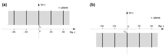
Figure 2. In the complex $\tau$-plane, the grey regions represent: (a) the cut-domain ${}^{\tau }{\mathcal{I}}_{+}^{\left({\xi }_0\right)}\setminus {}^{\tau }{\mathsf{\Xi }}_{+}^{\left({\xi }_0\right)}$, (b) the cut-domain ${}^{\tau }{\mathcal{I}}_{-}^{(-{\xi }_0)}\setminus {}^{\tau }{\mathsf{\Xi }}_{-}^{(-{\xi }_0)}$. The cuts (thick lines) are located at $\mathrm{Re}\tau =2k\pi$, $k\in \mathbb{Z}$.

Proposition 3.

Consider the trigonometric series

$$\frac{1}{2\pi }\sum _{n=0}^{+\infty }{a}_n{e}^{-\mathrm{i}n\tau }(\tau =t+\mathrm{i}w;t,w\in \mathbb{R}),$$

(26)

and suppose that the set of numbers ${\left\{f_n\right\}}_{n=0}^{\infty }$, with $f_n\doteq {(n+1)}^2{a}_n$, satisfies condition (20). Then:

(i) 

The series (26) converges uniformly on any compact subdomain of ${}^{\tau }{\mathcal{I}}_{-}^{\left(0\right)}$ to a function ${\widehat{f}}^{(+)}\left(\tau \right)$ holomorphic in ${}^{\tau }{\mathcal{I}}_{-}^{\left(0\right)}$, continuous on the axis $\mathrm{Im}\tau =0$.

(ii) 

The function ${\widehat{f}}^{(+)}\left(\tau \right)$ admits a holomorphic extension to the cut-domain ${}^{\tau }{\mathcal{I}}_{+}^{\left(0\right)}\setminus {}^{\tau }{\dot{\mathsf{\Xi }}}_{+}^{\left(0\right)}$: i.e., it is analytic in $\mathbb{C}\setminus \{\tau \in \mathbb{C}:\tau =2k\pi +\mathrm{i}w;k\in \mathbb{Z},w>0\}$.

(iii) 

The jump function ${\widehat{F}}^{(+)}\left(w\right)$, which is the discontinuity of $\left(\mathrm{i}{\widehat{f}}^{(+)}\left(\tau \right)\right)$ across the cut ${}^{\tau }{\dot{\mathsf{\Xi }}}_{+}^{\left(0\right)}$, is a function of class $C^1$ that satisfies the bound

$$\left|{\widehat{F}}^{(+)}\left(w\right)\right|⩽{∥{\tilde{a}}_{\sigma }∥}_1{e}^{\sigma w}\left(\sigma ⩾-\frac{1}{2},w\in {\mathbb{R}}^{+}\right),$$

where $\tilde{a}(\sigma +\mathrm{i}\mu )$ ($\mu \in \mathbb{R}$) is the unique Carlsonian interpolant of the coefficients $a_n$, and

$${∥{\tilde{a}}_{\sigma }∥}_1\doteq \frac{1}{2\pi }{\int }_{-\infty }^{+\infty }\left|\tilde{a}(\sigma +\mathrm{i}\mu )\right|\mathrm{d}\mu <\infty \left(\sigma ⩾-\frac{1}{2}\right).$$

(27)

(iv) 

${\widehat{F}}^{(+)}\left(w\right)=o\left(e^{-w/2}\right)$ for $w\to +\infty$ and ${\widehat{F}}^{(+)}\left(0\right)=0$.

(v) 

$\tilde{a}(\sigma +\mathrm{i}\mu )$ is the Laplace transform of the jump function ${\widehat{F}}^{(+)}\left(w\right)$:

$$\tilde{a}(\sigma +\mathrm{i}\mu )={\int }_0^{+\infty }{\widehat{F}}^{(+)}\left(w\right)e^{-(\sigma +\mathrm{i}\mu )w}\mathrm{d}w\left(\sigma >-\frac{1}{2}\right),$$

(28)

holomorphic in the half-plane $\sigma >-\frac{1}{2}$.

(vi) 

The following Plancherel equality holds:

$${\int }_{-\infty }^{+\infty }{\left|\tilde{a}(\sigma +\mathrm{i}\mu )\right|}^2\mathrm{d}\mu =2\pi {\int }_{-\infty }^{+\infty }{\left|{\widehat{F}}^{(+)}\left(w\right)e^{-\sigma w}\right|}^2\mathrm{d}w\left(\sigma ⩾-\frac{1}{2}\right).$$

Proof. 

Since the sequence ${\left\{f_n\right\}}_{n=0}^{\infty }$ satisfies condition (20), then, given an arbitrary constant C, there exists an integer $n_0$ such that $|a_n|⩽C$ for $n>n_0$ and, accordingly,

$$\left|\frac{1}{2\pi }\sum _{n=0}^{\infty }{a}_n{e}^{-\mathrm{i}n\tau }\right|⩽\frac{C}{2\pi }\sum _{n=n_0+1}^{\infty }{e}^{nw}(w\doteq \mathrm{Im}\tau ,C=\mathrm{constant}).$$

(29)

The series on the r.h.s. of (29) converges uniformly on any compact subdomain contained in the half-plane $w<0$. Since

$$\frac{1}{2\pi }\sum _{n=0}^{\infty }{a}_n{e}^{-\mathrm{i}n\tau }=\frac{1}{2\pi }\sum _{n=n_0+1}^{\infty }{a}_n{e}^{-\mathrm{i}n\tau }+T_{n_0}\left(\tau \right),$$

where $T_{n_0}\left(\tau \right)$ is a trigonometric polynomial, by the Weierstrass theorem on the uniformly convergent series of analytic functions, series (26) converges uniformly on any compact subdomain of ${}^{\tau }{\mathcal{I}}_{-}^{\left(0\right)}$ to a function ${\widehat{f}}^{(+)}\left(\tau \right)$ holomorphic in ${}^{\tau }{\mathcal{I}}_{-}^{\left(0\right)}$. Furthermore, since ${(n+1)}^2{a}_n\underset{n\to \infty }{\to }0$, given an arbitrary constant $C^{\prime }$, there exists an integer $n_1$ such that for $w=0$:

$$\left|\frac{1}{2\pi }\sum _{n=n_1}^{\infty }{a}_n{e}^{-\mathrm{i}nt}\right|⩽\frac{1}{2\pi }\sum _{n=n_1}^{\infty }\left|a_n\right|⩽\frac{C^{\prime }}{2\pi }\sum _{n=n_1}^{\infty }\frac{1}{n^2}⩽C^{\prime }\frac{\pi }{12}.$$

Then, applying once again the Weierstrass theorem on the uniformly convergent series of continuous functions, the series $\frac{1}{2\pi }{\sum }_{n=0}^{\infty }{a}_n{e}^{-\mathrm{i}nt}$ converges to a continuous function ${\widehat{f}}^{(+)}\left(t\right)$, and statement (i) is proved. Regarding statement (ii), we write the following integral:

$${\widehat{f}}_{\eta }^{(+)}\left(t\right)=\frac{\mathrm{i}}{4\pi }{\int }_{\mathcal{C}}\tilde{a}\left(\lambda \right)\frac{e^{-\mathrm{i}\lambda (t-\eta \pi )}}{sin\pi \lambda }\mathrm{d}\lambda (\eta =\pm ),$$

(30)

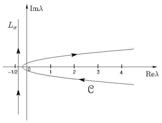
where $\tilde{a}\left(\lambda \right)$ ($\mathrm{Re}\lambda ⩾-\frac{1}{2}$) is the unique Carlsonian interpolant of the coefficients ${\left\{a_n\right\}}_{n=0}^{\infty }$, which is holomorphic in the half-plane $\mathrm{Re}\lambda >-\frac{1}{2}$ (see statement (i) of Proposition 2). The contour $\mathcal{C}$ is contained in the half-plane ${\mathbb{C}}_{-1/2}^{(+)}$, which encircles the semi-axis $\mathrm{Re}\lambda >-\frac{1}{2}$, and is chosen to cross the latter at a point $\sigma >-\frac{1}{2}$, $\sigma \notin \mathbb{N}$ (see Figure 3). Consider now the term $\frac{exp[-\mathrm{i}\lambda (t-\eta \pi \left)\right]}{sin\pi \lambda }$; the following inequalities hold ($\lambda =\sigma +\mathrm{i}\mu$):

$$\begin{array}{cc}\hfill & \left|e^{-\mathrm{i}(\sigma +\mathrm{i}\mu )(t-\eta \pi )}\right|⩽2cosh\pi \mu \mathrm{for}\left\{\begin{array}{cc}0⩽t⩽2\pi & \mathrm{if}\eta =+,\\ -2\pi ⩽t⩽0& \mathrm{if}\eta =-,\end{array}\right.\hfill \end{array}$$

(31)

$$\begin{array}{cc}\hfill & \left|sin\pi (\sigma +\mathrm{i}\mu )\right|⩾sinh\pi \mu ,\hfill \end{array}$$

(32)

$$\begin{array}{cc}\hfill & \left|sin\pi (\sigma +\mathrm{i}\mu )\right|⩾\left|sin\pi \sigma \right|cosh\pi \mu .\hfill \end{array}$$

(33)

Figure 3. Integration path of integral (30).

From (31) and (32):

$$\left|\frac{e^{-\mathrm{i}(\sigma +\mathrm{i}\mu )(t-\eta \pi )}}{sin\pi (\sigma +\mathrm{i}\mu )}\right|⩽2\left|\frac{cosh\pi \mu }{sinh\pi \mu }\right|\mathrm{for}\left\{\begin{array}{cc}0⩽t⩽2\pi & \mathrm{if}\eta =+,\\ -2\pi ⩽t⩽0& \mathrm{if}\eta =-,\end{array}\right.$$

(34)

while, combining (31) and (33):

$$\left|\frac{e^{-\mathrm{i}(\sigma +\mathrm{i}\mu )(t-\eta \pi )}}{sin\pi (\sigma +\mathrm{i}\mu )}\right|⩽\frac{2}{|sin\pi \sigma |}<\infty \mathrm{for}\left\{\begin{array}{cc}0⩽t⩽2\pi & \mathrm{if}\eta =+,\\ -2\pi ⩽t⩽0& \mathrm{if}\eta =-,\end{array}\right.\mathrm{and}\sigma \notin \mathbb{N}.$$

(35)

Integral (30) converges since ${\lambda }^2\tilde{a}\left(\lambda \right)$ tends uniformly to zero as $\lambda \to \infty$ in any fixed half-plane $\mathrm{Re}\lambda ⩾\delta >-\frac{1}{2}$ (statement (iii) of Proposition 2); the term $\left|\frac{exp[-\mathrm{i}(\sigma +\mathrm{i}\mu \left)\right(t-\eta \pi \left)\right]}{sin\pi (\sigma +\mathrm{i}\mu )}\right|$ is bounded by a constant for $\sigma \notin \mathbb{N}$ (see (35)), and is bounded by 2 as $\mu \to \pm \infty$ in view of inequality (34). The contour $\mathcal{C}$ can be distorted and replaced by a line $L_{\sigma }$ parallel to the imaginary axis and crossing the real axis at $\mathrm{Re}\lambda =\sigma$ with $\sigma ⩾-\frac{1}{2}$ ($\sigma \notin \mathbb{N}$) (see Figure 3) provided the real variable t is kept in $[0,2\pi ]$ for ${\widehat{f}}_{+}^{(+)}\left(t\right)$, and in $[-2\pi ,0]$ for ${\widehat{f}}_{-}^{(+)}\left(t\right)$, respectively. Note that the integral along $L_{\sigma }$ converges since $\lambda \tilde{a}\left(\lambda \right)\in L^1(-\infty ,+\infty )$ for any fixed value of $\mathrm{Re}\lambda ⩾-\frac{1}{2}$ (statement (iv) of Proposition 2) and by inequality (35). We may now apply the Watson resummation to integral (30). For $t\in [0,2\pi ]$, we obtain:

$$\frac{\mathrm{i}}{4\pi }{\int }_{\mathcal{C}}\tilde{a}\left(\lambda \right)\frac{e^{-\mathrm{i}\lambda (t-\pi )}}{sin\pi \lambda }\mathrm{d}\lambda =\frac{1}{2\pi }\sum _{n=0}^{\infty }{a}_n{e}^{-\mathrm{i}nt}\left(0⩽t⩽2\pi \right),$$

where the contour $\mathcal{C}$ encircles the semi-axis $\mathrm{Re}\lambda >-\frac{1}{2}$ and crosses it at a point $-\frac{1}{2}⩽\sigma <0$. Then, distorting the contour $\mathcal{C}$ into the line $L_{\sigma }$ ($-\frac{1}{2}⩽\sigma <0$), which is admissible as explained above, we obtain for $-\frac{1}{2}⩽\sigma <0$:

$${\widehat{f}}_{+}^{(+)}\left(t\right)=-\frac{1}{4\pi }{\int }_{-\infty }^{+\infty }\tilde{a}(\sigma +\mathrm{i}\mu )\frac{e^{-\mathrm{i}(\sigma +\mathrm{i}\mu )(t-\pi )}}{sin\pi (\sigma +\mathrm{i}\mu )}\mathrm{d}\mu =\frac{1}{2\pi }\sum _{n=0}^{\infty }{a}_n{e}^{-\mathrm{i}nt}\left(0⩽t⩽2\pi \right),$$

(36)

and, analogously, for $t\in [-2\pi ,0]$:

$${\widehat{f}}_{-}^{(+)}\left(t\right)=-\frac{1}{4\pi }{\int }_{-\infty }^{+\infty }\tilde{a}(\sigma +\mathrm{i}\mu )\frac{e^{-\mathrm{i}(\sigma +\mathrm{i}\mu )(t+\pi )}}{sin\pi (\sigma +\mathrm{i}\mu )}\mathrm{d}\mu =\frac{1}{2\pi }\sum _{n=0}^{\infty }{a}_n{e}^{-\mathrm{i}nt}\left(-2\pi ⩽t⩽0\right).$$

(37)

Now, substitute into integral (36) the real variable t with the complex variable $\tau =t+\mathrm{i}w$. The resulting integral can be proved to provide an analytic continuation of ${\widehat{f}}_{+}^{(+)}\left(t\right)$ in the strip $0<t<2\pi$, $w\in {\mathbb{R}}^{+}$, continuous in the closure of the latter. In fact, from the first equality in (36), we formally obtain:

$${\widehat{f}}_{+}^{(+)}(t+\mathrm{i}w)=\frac{1}{2\pi }{e}^{\sigma w}{\int }_{-\infty }^{+\infty }{H}_{\sigma }^t\left(\mu \right)e^{\mathrm{i}\mu w}\mathrm{d}\mu \left(0⩽t⩽2\pi ;w\in {\mathbb{R}}^{+},-\frac{1}{2}⩽\sigma <0\right),$$

(38)

where

$$H_{\sigma }^t\left(\mu \right)\doteq -\frac{\tilde{a}(\sigma +\mathrm{i}\mu )e^{-\mathrm{i}(\sigma +\mathrm{i}\mu )(t-\pi )}}{2sin\pi (\sigma +\mathrm{i}\mu )}.$$

(39)

By inequality (35) and statement (vi) of Proposition 2:

$$\left|H_{\sigma }^t\left(\mu \right)\right|⩽\frac{|\tilde{a}(-\frac{1}{2}+\mathrm{i}\mu )|}{|sin\pi \sigma |}\left(0⩽t⩽2\pi ;\sigma ⩾-\frac{1}{2},\sigma \notin \mathbb{N}\right),$$

(40)

which, along with statements (iv) and (v) of Proposition 2, guarantees that $H_{\sigma }^t\left(\mu \right)\in L^1(-\infty ,+\infty )$ for $0⩽t⩽2\pi ,\sigma >-\frac{1}{2},\sigma \notin \mathbb{N}$. Therefore, formulas (38), (39), and (40) define ${\widehat{f}}_{+}^{(+)}\left(\tau \right)$ ($\tau =t+\mathrm{i}w$) as an analytic continuation of ${\widehat{f}}_{+}^{(+)}\left(t\right)$ in the strip $\{\tau =t+\mathrm{i}w,0<t<2\pi ,w\in {\mathbb{R}}^{+}\}$, continuous in the closure of the latter in view of the Riemann–Lebesgue theorem. Proceeding analogously, we can obtain an analytic continuation of ${\widehat{f}}_{-}^{(+)}\left(t\right)$ in the strip $\{\tau =t+\mathrm{i}w,-2\pi <t<0,w\in {\mathbb{R}}^{+}\}$, continuous on the closure of the latter. It then follows that the function ${\widehat{f}}^{(+)}\left(\tau \right)$ admits a holomorphic extension to the cut-domain ${}^{\tau }{\mathcal{I}}_{+}^{\left(0\right)}{\setminus }^{\tau }{\dot{\mathsf{\Xi }}}_{+}^{\left(0\right)}$, and statement (ii) is proved.

The discontinuity ${\widehat{F}}^{(+)}\left(w\right)$ of $\left(\mathrm{i}{\widehat{f}}^{(+)}\left(\tau \right)\right)$ across the cut at $t=0$ equals $\mathrm{i}[{\widehat{f}}_{+}^{(+)}\left(\mathrm{i}w\right)-{\widehat{f}}_{-}^{(+)}\left(\mathrm{i}w\right)]$ ($w\in {\mathbb{R}}^{+}$) (for the $2\pi$-periodicity of ${\widehat{f}}^{(+)}\left(\tau \right)$, we may consider only the cut at $t=0$). It can be computed by replacing t by $\mathrm{i}w$ into integrals (36) and (37) and then subtracting Equation (37) from Equation (36):

$${\widehat{F}}^{(+)}\left(w\right)\doteq \mathrm{i}\left[{\widehat{f}}_{+}^{(+)}\left(\mathrm{i}w\right)-{\widehat{f}}_{-}^{(+)}\left(\mathrm{i}w\right)\right]=\frac{1}{2\pi }{\int }_{-\infty }^{+\infty }\tilde{a}(\sigma +\mathrm{i}\mu )e^{(\sigma +\mathrm{i}\mu )w}\mathrm{d}\mu \left(w\in {\mathbb{R}}^{+},\sigma ⩾-\frac{1}{2}\right),$$

(41)

which yields:

$$\left|{\widehat{F}}^{(+)}\left(w\right)\right|⩽{∥{\tilde{a}}_{\sigma }∥}_1{e}^{\sigma w}\left(w\in {\mathbb{R}}^{+},\sigma ⩾-\frac{1}{2}\right),$$

where ${∥{\tilde{a}}_{\sigma }∥}_1$, defined in (27), is guaranteed to be finite by statement (iv) of Proposition 2. Rewrite (41) as follows:

$${\widehat{F}}^{(+)}\left(w\right)e^{-\sigma w}=\frac{1}{2\pi }{\int }_{-\infty }^{+\infty }\tilde{a}(\sigma +\mathrm{i}\mu )e^{\mathrm{i}\mu w}\mathrm{d}\mu \left(w\in {\mathbb{R}}^{+},\sigma ⩾-\frac{1}{2}\right).$$

(42)

Since for any fixed $\mathrm{Re}\lambda ⩾-\frac{1}{2}$, $\lambda \tilde{a}\left(\lambda \right)$ and $\tilde{a}\left(\lambda \right)$ belong to $L^1(-\infty ,+\infty )$, the Riemann–Lebesgue theorem guarantees that ${\widehat{F}}^{(+)}\left(w\right)e^{-\sigma w}$ is a function of class $C^1$ tending to zero as $w\to +\infty$, and statement (iii) is proved. Hence, ${\widehat{F}}^{(+)}\left(w\right)$ is a continuous function of w ($w\in {\mathbb{R}}^{+}$) and ${\widehat{F}}^{(+)}\left(w\right)=o\left(e^{-w/2}\right)$ as $w\to +\infty$. Moreover, ${\widehat{F}}^{(+)}\left(0\right)=0$ for the continuity of ${\widehat{f}}^{(+)}\left(\tau \right)$ on the real axis, and statement (iv) is proved. Inverting (42), we have:

$$\tilde{a}(\sigma +\mathrm{i}\mu )={\int }_0^{+\infty }{\widehat{F}}^{(+)}\left(w\right)e^{-(\sigma +\mathrm{i}\mu )w}\mathrm{d}w\left(\sigma >-\frac{1}{2}\right),$$

where the integral on the r.h.s. converges for $\sigma >-\frac{1}{2}$. It defines the Laplace transform of ${\widehat{F}}^{(+)}\left(w\right)$, holomorphic in the half-plane $\mathrm{Re}\lambda >-\frac{1}{2}$, and statement (v) follows. Finally, recalling that $\tilde{a}(\sigma +\mathrm{i}\mu )$ ($\mu \in \mathbb{R}$) belongs to $L^2(-\infty ,+\infty )$ for any fixed value $\sigma ⩾-\frac{1}{2}$ (statement (ii) of Proposition 2 and inequality (25)), we obtain the Plancherel equality:

$${\int }_{-\infty }^{+\infty }{\left|\tilde{a}\left(\sigma +\mathrm{i}\mu \right)\right|}^2\mathrm{d}\mu =2\pi {\int }_0^{+\infty }{\left|{\widehat{F}}^{(+)}\left(w\right)e^{-\sigma w}\right|}^2\mathrm{d}w\left(\sigma ⩾-\frac{1}{2}\right),$$

proving statement (vi). □

Proposition 4.

If in the trigonometric series (see (19))

$$\frac{1}{2\pi }\left[\sum _{n=0}^{\infty }{a}_n{e}^{-\mathrm{i}nt}-e^{\mathrm{i}t}\sum _{n=0}^{\infty }{a}_n{e}^{\mathrm{i}nt}\right](t\in \mathbb{R}),$$

(43)

the coefficients $a_n$ satisfy the assumptions required by Propositions 2 and 3, i.e., the set of numbers $f_n={(n+1)}^2{a}_n$ satisfies condition (20), then:

(i) 

The series (43) converges to a continuous function $\widehat{f}\left(t\right)$ ($t\in \mathbb{R}$).

(ii) 

The function $\widehat{f}\left(t\right)$ admits a holomorphic extension to the cut-domain ${(}^{\tau }{\mathcal{I}}_{+}^{\left(0\right)}\setminus {}^{\tau }{\dot{\mathsf{\Xi }}}_{+}^{\left(0\right)})\cup ({}^{\tau }{\mathcal{I}}_{-}^{\left(0\right)}\setminus {}^{\tau }{\dot{\mathsf{\Xi }}}_{-}^{\left(0\right)})$, i.e., it is analytic in $\mathbb{C}\setminus \{\tau =2k\pi +\mathrm{i}w;k\in \mathbb{Z},w\in \mathbb{R},w\ne 0\}$.

(iii) 

The jump function across the cuts ${}^{\tau }{\dot{\mathsf{\Xi }}}_{\pm }^{\left(0\right)}$ enjoys properties, mutatis mutandis, analogous to conditions (iii)–(vi) of Proposition 3.

Proof. 

These statements can be proved by using obvious extensions of the arguments used in the proof of Proposition 3. □

Through the holomorphic extension associated with the trigonometric series (43), we obtain a function, denoted by $\widehat{f}\left(\tau \right)$ ($\tau =t+\mathrm{i}w;t,w\in \mathbb{R}$), which is the analytic continuation of $\widehat{f}\left(t\right)$ ($t\in \mathbb{R}$) from the real axis to the domain ${}^{\tau }\dot{\mathcal{I}}\doteq ({}^{\tau }{\mathcal{I}}_{+}^{\left(0\right)}\setminus {}^{\tau }{\dot{\mathsf{\Xi }}}_{+}^{\left(0\right)})\cup ({}^{\tau }{\mathcal{I}}_{-}^{\left(0\right)}\setminus {}^{\tau }{\dot{\mathsf{\Xi }}}_{-}^{\left(0\right)})$. We can then prove the following corollary to Proposition 4.

Corollary 1.

The function $\widehat{f}\left(\tau \right)$ is holomorphic in the $2\pi$-periodic strips ${\mathsf{\Sigma }}_{\tau }\doteq \{\tau \in \mathbb{C}:\tau =t+\mathrm{i}w,2\pi k<t<2\pi (k+1),k\in \mathbb{Z},w\in \mathbb{R}\}$.

Proof. 

We start from statement (ii) of Proposition 4. Next, by applying the Schwarz reflection principle and taking into account that the function $\widehat{f}\left(t\right)$ (i.e., the restriction of $\widehat{f}\left(\tau \right)$ to the real axis) is continuous (statement (i) of Proposition 4), the statement of the corollary follows. □

Remark 2.

In Ref. [21], the Hausdorff condition (20) was assumed to hold for the set of numbers $f_n=n^p{a}_n$ ($p⩾2$). However, this condition does not guarantee obtaining a unique Carlsonian interpolation of the whole sequence $a_n$, including the first coefficient $a_0$. Therefore, it must be replaced by the same condition on the numbers $f_n={(n+1)}^p{a}_n$ ($p⩾2$). However, for the purpose of the current analysis, it is sufficient to take $p=2$. Let us note that the results of Ref. [21] hold true and, in particular, the proofs of Propositions 5.1 and 6.1 of that paper, which will be used below, are correct modulo the following change: $f_n=n^p{a}_n\to f_n={(n+1)}^p{a}_n$.

2.4. Inversion of the Radon–Abel Transformation and Holomorphic Extension Associated with the Legendre Series

The first step consists of determining the inversion of the Radon–Abel transformation (12). We can prove the following proposition.

Proposition 5.

Suppose that the sequence $f_n={(n+1)}^2{a}_n$ ($a_n$ being the coefficients of the Legendre expansion (14)) satisfies the Hausdorff condition (20). Then, the Radon–Abel transformation (see (12))

$$\widehat{f}\left(t\right)=-2e^{\mathrm{i}t/2}{\int }_0^{t}f\left(u\right)\frac{sinu}{{\left[2(cost-cosu)\right]}^{\frac{1}{2}}}\mathrm{d}u$$

(44)

admits the following inversion:

$$f\left(u\right)=\frac{1}{\pi sinu}\frac{\mathrm{d}}{\mathrm{d}u}{\int }_0^u{e}^{-\mathrm{i}t/2}\widehat{f}\left(t\right)\frac{sint}{{\left[2(cosu-cost)\right]}^{\frac{1}{2}}}\mathrm{d}t.$$

Proof. 

See Proposition 5.1 of Ref. [21]. □

By following the same procedure used in the proof of Proposition 5 (i.e., introducing Riemann–Liouville integrals and related properties), Proposition 5 can be extended to give the inversion of the Radon–Abel transformation (11). We can state, without proof, the following proposition.

Proposition 6.

Assume that the coefficients $a_n$ (see (14)) satisfy the conditions of Proposition 5; then, the function $\widehat{f}\left(\tau \right)$, i.e., the analytic continuation of the function $\widehat{f}\left(t\right)$ given in (44), is holomorphic in the strips ${\mathsf{\Sigma }}_{\tau }$ and can be represented by the following Radon–Abel transformation (see (11)):

$$\widehat{f}\left(\tau \right)=-2e^{\mathrm{i}\tau /2}{\int }_{{\gamma }_{\tau }}f\left(\theta \right)\frac{sin\theta }{{\left[2(cos\tau -cos\theta )\right]}^{\frac{1}{2}}}\mathrm{d}\theta ,$$

which admits the following inversion:

$$f\left(\theta \right)=\frac{1}{\pi sin\theta }\frac{\mathrm{d}}{\mathrm{d}\theta }{\int }_{{\gamma }_{\theta }}{e}^{-\mathrm{i}\tau /2}\widehat{f}\left(\tau \right)\frac{sin\tau }{{\left[2(cos\theta -cos\tau )\right]}^{\frac{1}{2}}}\mathrm{d}\tau ,$$

(45)

${\gamma }_{\tau }$ and ${\gamma }_{\theta }$ denoting the rays from zero to τ and from zero to θ, respectively.

We can now prove the following proposition.

Proposition 7.

Suppose that the sequence $f_n={(n+1)}^2{a}_n$ ($n=0,1,2,\dots$) satisfies the Hausdorff condition (20), then the function $f\left(\theta \right)$ ($\theta \in \mathbb{C}$), represented by formula (45), is even, $2\pi$-periodic, and holomorphic in ${}^{\theta }\dot{\mathcal{I}}=({}^{\theta }{\mathcal{I}}_{+}^{\left(0\right)}\setminus {}^{\theta }{\dot{\mathsf{\Xi }}}_{+}^{\left(0\right)})\cup ({}^{\theta }{\mathcal{I}}_{-}^{\left(0\right)}\setminus {}^{\theta }{\dot{\mathsf{\Xi }}}_{-}^{\left(0\right)})$.

Proof. 

The assumptions on the Legendre coefficients $a_n$ allow us to state that $\widehat{f}\left(\tau \right)$ is a $2\pi$-periodic function, holomorphic in the domain ${}^{\tau }\dot{\mathcal{I}}$ (see Corollary 1). Moreover, it enjoys the symmetry property:

$$\widehat{f}\left(\tau \right)=-e^{\mathrm{i}\tau }\widehat{f}(-\tau ),$$

which follows from (17) and from the uniqueness of the analytic continuation. The properties mentioned above imply that $\widehat{f}\left(\tau \right)$ is of the form: $\widehat{f}\left(\tau \right)=e^{\mathrm{i}\tau /2}{(1-cos\tau )}^{\frac{1}{2}}b(cos\tau )$, with $b(cos\tau )$ analytic in ${}^{\tau }\underline{D}=\{cos\tau \in \mathbb{C},\tau \in {}^{\tau }\dot{\mathcal{I}}\}$. Through the following parametrization of ${\gamma }_{\theta }$: $cos\tau =1+\delta (cos\theta -1)$, ($0⩽\delta ⩽1$), formula (45) can be rewritten as:

$$f\left(\theta \right)=\frac{\mathrm{i}}{\sqrt{2}\pi }\frac{\mathrm{d}}{\mathrm{d}(cos\theta )}\left[(cos\theta -1){\int }_0^{1}b(1+\delta (cos\theta -1)){\delta }^{\frac{1}{2}}{(1-\delta )}^{-\frac{1}{2}}\mathrm{d}\delta \right],$$

which represents a function holomorphic in ${}^{\theta }\underline{D}=\{cos\theta \in \mathbb{C},\theta \in {}^{\theta }\dot{\mathcal{I}}\}$. Accordingly, regarded as a function of $\theta$, it represents an even function, $2\pi$-periodic, and holomorphic in ${}^{\theta }\dot{\mathcal{I}}$. □

From the previous proposition and Corollary 1, it derives the following corollary.

Corollary 2.

If the sequence ${\left\{a_n\right\}}_{n=0}^{\infty }$ of the Legendre coefficients satisfies the conditions of Proposition 7, then $f\left(\theta \right)$ is a function analytic in the $2\pi$-periodic strips ${\mathsf{\Sigma }}_{\theta }\doteq \{\theta \in \mathbb{C}:\theta =u+\mathrm{i}v,2\pi k<u<2\pi (k+1),k\in \mathbb{Z},v\in \mathbb{R}\}$.

Formula (45) allows us to compute the boundary values $f_{\pm }^{(+)}\left(\mathrm{i}v\right)$, which are defined by $f_{\eta }^{(+)}\left(v\right)\doteq {lim}_{u\to 0^{+}}{f}^{(+)}(\eta u+\mathrm{i}v),\eta =\pm ,v⩾0$, on the semi-axis $\theta =\mathrm{i}v$, $v⩾0$, with ${\gamma }_{\mathrm{i}v}=\{\tau =\mathrm{i}w,0⩽w⩽v\}$, in terms of the corresponding boundary values ${\widehat{f}}_{\pm }^{(+)}\left(\mathrm{i}w\right)$, provided ${\widehat{f}}_{\pm }^{(+)}\left(\mathrm{i}w\right)$ satisfies a $C^1$-type regularity condition; the latter condition is necessary in order to perform the inversion of the Radon–Abel transform at the boundary. The $C^1$-continuity of the boundary values follows from the fact that the sequence $f_n={(n+1)}^2{a}_n$ is required to satisfy the Hausdorff condition (20) (see Propositions 2 and 3). We thus obtain:

$$F^{(+)}\left(v\right)\doteq \mathrm{i}[f_{+}^{(+)}\left(\mathrm{i}v\right)-f_{-}^{(+)}\left(\mathrm{i}v\right)]=\frac{1}{\pi sinhv}\frac{\mathrm{d}}{\mathrm{d}v}{\int }_0^v{e}^{w/2}{\widehat{F}}^{(+)}\left(w\right)\frac{sinhw}{{\left[2(coshv-coshw)\right]}^{\frac{1}{2}}}\mathrm{d}w,$$

(46)

where ${\widehat{F}}^{(+)}\left(w\right)\doteq \mathrm{i}[{\widehat{f}}_{+}^{(+)}\left(\mathrm{i}w\right)-{\widehat{f}}_{-}^{(+)}\left(\mathrm{i}w\right)]$, ${\widehat{f}}_{\eta }^{(+)}\left(\mathrm{i}w\right)={lim}_{t\to 0^{+}}{\widehat{f}}^{(+)}(\eta t+\mathrm{i}w),\eta =\pm$. At this point, let us note that, for the current analysis, it is sufficient to consider the cuts in the $\tau$- and $\theta$-planes at $\tau =2k\pi +\mathrm{i}w$ ($k\in \mathbb{Z},w>0$) and $\theta =2k\pi +\mathrm{i}v$ ($k\in \mathbb{Z},v>0$), respectively. Therefore, we can limit ourselves to consider the functions: ${\widehat{F}}^{(+)}\left(w\right)=e^{-v/2}\left(\mathcal{A}F\right)\left(w\right)$ ($w⩾0$) and, correspondingly, $F^{(+)}\left(v\right)\equiv {\underline{F}}^{(+)}(coshv)$ ($v⩾0$). For simplicity, hereafter we shall omit the superscript $(+)$ in these notations.

Next, we can apply the inverse Radon–Abel operator (defined by (45)) to the series on the r.h.s. of formula (19), i.e.,

$$\widehat{f}\left(t\right)=\frac{1}{2\pi }{e}^{\mathrm{i}(t-\pi )/2}\sum _{n=-\infty }^{+\infty }{(-1)}^n{a}_{n}cos\left[\left(n+\frac{1}{2}\right)(t-\pi )\right],$$

whose term by term integration is legitimate for the uniform convergence of the series, which follows from the Hausdorff conditions satisfied by the coefficients $\left\{a_n\right\}$. We now introduce the functions

$${\psi }_n(cosu)\doteq -\frac{\mathrm{i}}{\pi sinu}\frac{\mathrm{d}}{\mathrm{d}u}{\int }_0^{u}cos\left[\left(n+\frac{1}{2}\right)(t-\pi )\right]\frac{sint}{{\left[2(cosu-cost)\right]}^{\frac{1}{2}}}\mathrm{d}t(0<u<2\pi ),$$

which are related to the Legendre polynomials $P_n(cosu)$ by [21]:

$${\psi }_n(cosu)=\frac{{(-1)}^n}{4}(2n+1)P_n(cosu).$$

Recalling that $a_n=-a_{-n-1}$ ($n\in \mathbb{Z}$) (formula (18)), we finally obtain the original Legendre expansion

$$f\left(u\right)=\underline{f}(cosu)=\frac{1}{\pi }\sum _{n=0}^{\infty }{(-1)}^n{a}_n{\psi }_n(cosu)=\frac{1}{4\pi }\sum _{n=0}^{\infty }(2n+1)a_n{P}_n(cosu).$$

All the results obtained for the function $\underline{f}(cos\theta )$ in the $cos\theta$-plane can be summarized in the following theorem.

Theorem 2.

If the sequence $f_n={(n+1)}^2{a}_n$ ($n=0,1,2,\dots$) satisfies the Hausdorff condition (20), then:

(i) 

Series (14) converges to a function $\underline{f}(cosu)$ ($u\equiv \mathrm{Re}\theta$), analytic in the interval $-1<cosu<1$.

(ii) 

The function $\underline{f}(cosu)$ admits a holomorphic extension to the complex $cos\theta$-plane ($\theta =u+\mathrm{i}v$) cut along the semi-axis $[1,+\infty )$.

2.5. Spherical Laplace Transform and Analyticity Properties in the Complex $\lambda$-Plane

A basic feature of the holomorphic extensions associated with the series expansions is the dual analyticity that we shall illustrate in the specific case that we have considered here, of the Legendre series (14). To classes of functions $\underline{f}(cos\theta )$ holomorphic in the $cos\theta$-plane cut along the semi-axis $[1,+\infty )$ (see Theorem 2), there correspond classes of analytic functions $\tilde{a}\left(\lambda \right)$ ($\lambda \in \mathbb{C}$), which enjoy the following properties:

(a)

$\tilde{a}\left(\lambda \right)$ is the composition of the standard Laplace transform with the Abel transform (multiplied by the factor $e^{-w/2}$) of the jump function of $\left[\mathrm{i}\widehat{f}\left(\theta \right)\right]$ across the cut ${}^{\theta }{\dot{\mathsf{\Xi }}}_{+}^{\left(0\right)}$, that is, the spherical Laplace transform.

(b)

$\tilde{a}\left(\lambda \right)$ is holomorphic in the half-plane $\mathrm{Re}\lambda >-\frac{1}{2}$.

(c)

$\tilde{a}\left(\lambda \right)$ is the (unique) Carlsonian interpolant of the Fourier–Legendre coefficients: $\tilde{a}{\left(\lambda \right)|}_{\lambda =n}=a_n$.

Formulas (9) and (28) give

$$\tilde{a}\left(\lambda \right)={\int }_0^{+\infty }{e}^{-(\lambda +\frac{1}{2})w}\left(\mathcal{A}F\right)\left(w\right)\mathrm{d}w\left(\mathrm{Re}\lambda >-\frac{1}{2}\right),$$

which is precisely the spherical Laplace transform, holomorphic in the half-plane $\mathrm{Re}\lambda >-\frac{1}{2}$ (statement (v) of Proposition 3). Moreover, $\tilde{a}{\left(\lambda \right)|}_{\lambda =n}=a_n$ (statement (i) of Proposition 2). Writing explicitly the Abel transform $\left(\mathcal{A}F\right)\left(w\right)$ (see (9)), we obtain

$$\tilde{a}\left(\lambda \right)=2{\int }_0^{+\infty }{e}^{-(\lambda +\frac{1}{2})w}\left\{{\int }_0^w\underline{F}(coshv)\frac{sinhv}{{\left[2(coshw-coshv)\right]}^{\frac{1}{2}}}\mathrm{d}v\right\}\mathrm{d}w\left(\mathrm{Re}\lambda >-\frac{1}{2}\right),$$

which, interchanging the order of integration, becomes

$$\tilde{a}\left(\lambda \right)=2{\int }_0^{+\infty }\underline{F}(coshv)sinhv\left\{{\int }_v^{+\infty }\frac{e^{-(\lambda +\frac{1}{2})w}}{{\left[2(coshw-coshv)\right]}^{\frac{1}{2}}}\mathrm{d}w\right\}\mathrm{d}v\left(\mathrm{Re}\lambda >-\frac{1}{2}\right).$$

(47)

Using the integral representation of the Legendre functions of the second kind [24]

$$Q_{\lambda }(coshv)={\int }_v^{+\infty }\frac{e^{-(\lambda +\frac{1}{2})w}}{{\left[2(coshw-coshv)\right]}^{\frac{1}{2}}}\mathrm{d}w\left(\mathrm{Re}\lambda >-1,v>0\right),$$

(48)

formula (47) can be written as follows:

$$\tilde{a}\left(\lambda \right)=2{\int }_0^{+\infty }\underline{F}(coshv)Q_{\lambda }(coshv)sinhv\mathrm{d}v\left(\mathrm{Re}\lambda >-\frac{1}{2}\right).$$

(49)

Remark 3.

The Legendre function of the second kind has a logarithmic singularity at $v=0$, then the integral representation (48) holds if $v>0$; nevertheless, the integral in (49) converges if $\underline{F}(coshv)$ is regular at $v=0$.

We can now state the following theorem.

Theorem 3.

If the sequence $f_n={(n+1)}^2{a}_n$ ($n=0,1,2,\dots$), $a_n$ being the Legendre coefficients of expansion (14), satisfies the Hausdorff condition (20), then the jump function $F\left(v\right)=\underline{F}(coshv)$ (defined in (46)) admits the following integral representation:

$$\begin{array}{c}F\left(v\right)=\underline{F}(coshv)=\frac{1}{2\pi }{\int }_{-\infty }^{+\infty }\tilde{a}(\sigma +\mathrm{i}\mu )\left(\sigma +\frac{1}{2}+\mathrm{i}\mu \right)P_{\sigma +\mathrm{i}\mu }(coshv)\mathrm{d}\mu \hfill \\ =\frac{1}{2\pi \mathrm{i}}{\int }_{\sigma -\mathrm{i}\infty }^{\sigma +\mathrm{i}\infty }\tilde{a}\left(\lambda \right)\left(\lambda +\frac{1}{2}\right)P_{\lambda }(coshv)\mathrm{d}\lambda \left(\lambda =\sigma +\mathrm{i}\mu ;\sigma ⩾-\frac{1}{2}\right),\hfill \end{array}$$

(50)

where $P_{\lambda }(·)$ denotes the Legendre function of the first kind.

Proof. 

See Proposition 6.1 of Ref. [21]. □

3. From Spherical Laplace Transform to Non-Euclidean Fourier Transform

3.1. Formal Derivation of Mehler’s Transform from the Spherical Laplace Transform

Let us begin by considering the integral representation (48) of the Legendre function of the second kind $Q_{\lambda }(coshv)$. If $\mathrm{Re}\lambda =-\frac{1}{2}$, the function $Q_{-\frac{1}{2}+\mathrm{i}\mu }(coshv)$ can be written as the sum of its even (in $\mu$) and odd parts, which are defined as follows:

$$\begin{array}{cc}\hfill Q_{-\frac{1}{2}+\mathrm{i}\mu }^{\left(\mathrm{E}\right)}(coshv)=& {\int }_v^{+\infty }\frac{cos\mu w}{{\left[2(coshw-coshv)\right]}^{\frac{1}{2}}}\mathrm{d}w,\hfill \\ \hfill Q_{-\frac{1}{2}+\mathrm{i}\mu }^{\left(\mathrm{O}\right)}(coshv)=& -\mathrm{i}{\int }_v^{+\infty }\frac{sin\mu w}{{\left[2(coshw-coshv)\right]}^{\frac{1}{2}}}\mathrm{d}w.\hfill \end{array}$$

Recalling the relation between the Legendre functions of first and second kind (p. 140, [24])

$$P_{\lambda }\left(z\right)=\frac{tan\pi \lambda }{\pi }\left[Q_{\lambda }\left(z\right)-Q_{-\lambda -1}\left(z\right)\right],$$

and exploiting the evenness (in $\mu$) of the conical Legendre functions, i.e., $P_{-\frac{1}{2}+\mathrm{i}\mu }(coshv)=P_{-\frac{1}{2}-\mathrm{i}\mu }(coshv)$ ($\mu \in \mathbb{R}$), we obtain:

$$P_{-\frac{1}{2}+\mathrm{i}\mu }(coshv)=P_{-\frac{1}{2}-\mathrm{i}\mu }(coshv)=\frac{2}{\pi }tan\left[\pi \left(-\frac{1}{2}+\mathrm{i}\mu \right)\right]Q_{-\frac{1}{2}+\mathrm{i}\mu }^{\left(\mathrm{O}\right)}(coshv).$$

(51)

Let us now return to Theorem 3 and to formula (50) in the specific case $\sigma =-\frac{1}{2}$. By the $\mu$-evenness of $P_{-\frac{1}{2}+\mathrm{i}\mu }(coshv)$, it follows that only the odd component ${\tilde{a}}^{\left(\mathrm{O}\right)}(-\frac{1}{2}+\mathrm{i}\mu )$ of $\tilde{a}(-\frac{1}{2}+\mathrm{i}\mu )$ ($\mu \in \mathbb{R}$) contributes to the integral in formula (50):

$$F\left(v\right)=\underline{F}(coshv)=\frac{\mathrm{i}}{\pi }{\int }_0^{+\infty }{\tilde{a}}^{\left(\mathrm{O}\right)}\left(-\frac{1}{2}+\mathrm{i}\mu \right)P_{-\frac{1}{2}+\mathrm{i}\mu }(coshv)\mu \mathrm{d}\mu .$$

(52)

Moving back to formula (49), which for the moment we assume to hold also for $\mathrm{Re}\lambda =-\frac{1}{2}$ (this statement will be proved later in Section 3.4.3), and accounting for relationship (51), we can formally rewrite the odd component of $\tilde{a}(-\frac{1}{2}+\mathrm{i}\mu )$ ($\mu \in \mathbb{R}$) as follows:

$${\tilde{a}}^{\left(\mathrm{O}\right)}\left(-\frac{1}{2}+\mathrm{i}\mu \right)=\frac{\pi }{tan\left[\pi \left(-\frac{1}{2}+\mathrm{i}\mu \right)\right]}{\int }_0^{+\infty }\underline{F}(coshv)P_{-\frac{1}{2}+\mathrm{i}\mu }(coshv)sinhv\mathrm{d}v(\mu \in \mathbb{R}).$$

(53)

Noting that ${(tan\left[\pi (-\frac{1}{2}+\mathrm{i}\mu )\right])}^{-1}=-\mathrm{i}tanh\pi \mu$, we may introduce the following function: $\tilde{F}\left(\mu \right)\doteq \tilde{a}(-\frac{1}{2}+\mathrm{i}\mu )/(-\mathrm{i}\pi tanh\pi \mu )$ (we omit here the superscript “$\left(\mathrm{O}\right)$” in ${\tilde{a}}^{\left(\mathrm{O}\right)}\left(-\frac{1}{2}+\mathrm{i}\mu \right)$ since only the odd part of $\tilde{a}(-\frac{1}{2}+\mathrm{i}\mu )$ plays a role in these transformations). Then, formulas (52) and (53) can be rewritten as

$$\begin{array}{cc}\hfill F\left(v\right)& =\underline{F}(coshv)={\int }_0^{+\infty }\tilde{F}\left(\mu \right)P_{-\frac{1}{2}+\mathrm{i}\mu }(coshv)tanh\left(\pi \mu \right)\mu \mathrm{d}\mu ,\hfill \end{array}$$

(54a)

$$\begin{array}{cc}\hfill \tilde{F}\left(\mu \right)& ={\int }_0^{+\infty }\underline{F}(coshv)P_{-\frac{1}{2}+\mathrm{i}\mu }(coshv)sinhv\mathrm{d}v,\hfill \end{array}$$

(54b)

which coincide with the Mehler transform pair, indeed (see (p. 175, [24])).

Remark 4.

(i) As we have already remarked above, we do not consider the whole spherical Laplace transform but only its odd (with respect to μ) component since only this component plays a role in the transformations being treated here.

(ii) The class of functions $F\left(v\right)$ which we are led to consider here are of the form $\underline{F}=\underline{F}(coshv)$. Accordingly, the connection between spherical Laplace transform and non-Euclidean Fourier transform can be limited to this class of functions. In the non-Euclidean geometry, these functions belong to the class of radial functions in a sense that will be clarified in what follows (see Remarks 5 and 6).

3.2. Geometry of the Two-Sheeted Hyperboloid: Polar and Horocyclic Coordinates

Let us now return to the geometrical representation of the real one-sheeted hyperboloid $X_2$. It can be easily noted that, by simply swapping two coordinate axes (see Figure 1 and Figure 4), the real meridian ${\widehat{X}}^{+}$ can be regarded as the real meridian of one of the sheets of a suitable real two-sheeted hyperboloid. It is therefore reasonable to expect that an integral representation of $\underline{F}(coshv)$ can be obtained also from the geometry of the two-sheeted hyperboloid.

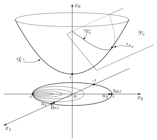
Figure 4. Upper sheet ${}^2{X}_2^{+}$ of the real two-sheteed hyperboloid. $\mathrm{Re}z$ is directed along $u_1$ and $\mathrm{Im}z$ along $u_2$.

In the space ${\mathbb{R}}^3$ of variables $x=(x_0,x_1,x_2)$, we consider the two-sheeted hyperboloid with equation:

$$x_0^2-x_1^2-x_2^2=1.$$

(55)

In the present analysis, we can limit ourselves to consider the upper sheet of this two-sheeted hyperboloid, the one with $x_0⩾1$ that will be denoted by ${}^2{X}_2^{+}$. By analogy with what we have done is Section 2, we consider two systems of coordinates: polar and horocyclic coordinates.

Polar Coordinates:

$$\begin{array}{cc}\hfill x_0& =coshv,\hfill \end{array}$$

(56a)

$$\begin{array}{cc}\hfill x_1& =sinhvsin\psi ,(v⩾0,\psi \in [0,2\pi \left)\right),\hfill \end{array}$$

(56b)

$$\begin{array}{cc}\hfill x_2& =sinhvcos\psi .\hfill \end{array}$$

(56c)

It is easy to verify that $x_0^2-x_1^2-x_2^2={cosh}^{2}v-{sinh}^{2}v=1$, and $x_0⩾1$.

Horocyclic Coordinates:

$$\begin{array}{cc}\hfill x_0& =coshw+\frac{1}{2}{\zeta }^2{e}^w,\hfill \end{array}$$

(57a)

$$\begin{array}{cc}\hfill x_1& =\zeta e^w,(w,\zeta \in \mathbb{R}),\hfill \end{array}$$

(57b)

$$\begin{array}{cc}\hfill x_2& =sinhw-\frac{1}{2}{\zeta }^2{e}^w.\hfill \end{array}$$

(57c)

Even in this case, it is straightforward to verify that $x_0^2-x_1^2-x_2^2=1$, and $x_0⩾1$; accordingly, the horocyclic coordinates (57) are appropriate for describing the upper sheet ${}^2{X}_2^{+}$ of the real two-sheeted hyperboloid. In particular, we focus our attention on the meridian section ${}^2{\widehat{X}}^{+}$ of the upper sheet ${}^2{X}_2^{+}$, which lies in the plane $x_1=0$ and whose equation is $x_0^2-x_2^2=1$. We consider the intersections of ${}^2{\widehat{X}}^{+}$ with the family of planes ${}^2{P}_w$ with equation $x_0+x_2=e^w$ ($w\in \mathbb{R}$), i.e., the points ${}^2{x}_w$, whose coordinates are $x_0=coshw$, $x_1=0$, $x_2=sinhw$. The sections of ${}^2{X}_2^{+}$ by these planes are the (real) parabolae ${}^2{\mathsf{\Pi }}_w^{+}$. Setting $\zeta =0$ in (57), we obtain the point ${}^2{x}_w$ ($w\in \mathbb{R}$), which is the apex of the corresponding parabola ${}^2{\mathsf{\Pi }}_w^{+}$ (see Figure 4).

Remark 5.

As we shall see in the next section, the parabolae ${}^2{\mathsf{\Pi }}_w^{+}$ generate (through a stereographic projection on the non-Euclidean disk) a family of horocycles, represented by the Euclidean circles (illustrated in Figure 4) which are tangent to the boundary of the unit disk at the point $x_1=0,x_2=-1$. It is worth emphasizing that this is the sole family of horocycles which is generated by the fibration illustrated above. On the other hand, the non-Euclidean Fourier transform, which will be studied in the next section, demands considering in the non-Euclidean disk all the families of horocycles which are obtained by moving the point of tangency along the entire horizon from 0 to $2\pi$. We shall see in Lemma 2 of Section 3.4.1 how this difficulty will be overcome (see also Remark 6).

3.3. Stereographic Projection from the Upper Sheet of the Two-Sheeted Hyperboloid to the Non-Euclidean Unit Disk

Let $u=(u_1,u_2)$ denote the Cartesian coordinate system in the open unit disk $D\doteq \{u:u_1^1+u_2^2<1\}$, which lies in the plane $x_0=0$:

$$\begin{array}{cc}\hfill u_1& =tanh\left(\frac{v}{2}\right)sin\psi (v⩾0,\psi \in [0,2\pi )),\hfill \end{array}$$

(58a)

$$\begin{array}{cc}\hfill u_2& =tanh\left(\frac{v}{2}\right)cos\psi .\hfill \end{array}$$

(58b)

Then: ${\left|u\right|}^2=u_1^2+u_2^2={tanh}^2(v/2)$. Let $B\doteq \{u:u_1^1+u_2^2=1\}$ denote the boundary of D, i.e., the horizon. Consider the Riemannian structure

$$\mathrm{d}{s}^2=\frac{4(\mathrm{d}{u}_1^2+\mathrm{d}{u}_2^2)}{{[1-(u_1^2+u_2^2)]}^2}=\mathrm{d}{v}^2+{sinh}^{2}v\mathrm{d}{\psi }^2,$$

(59)

where $\mathrm{d}{v}^2+{sinh}^{2}v\mathrm{d}{\psi }^2$ can also be obtained from (56) through the equality: $\mathrm{d}{s}^2=-\mathrm{d}{x}_0^2+\mathrm{d}{x}_1^2+\mathrm{d}{x}_2^2$. Let us embed the non-Euclidean disk in the complex z-plane so that each point of the unit disk can be represented either by the coordinates $(u_1,u_2)$ in (58) or through the polar representation of z, which in the present case reads: $z=\left|z\right|exp\left[\mathrm{i}(\frac{\pi }{2}-\psi )\right]$, $\left|z\right|=tanh\left(\frac{v}{2}\right)$. Note that in this latter representation we are forced to write $exp\left[\mathrm{i}(\frac{\pi }{2}-\psi )\right]$ with $\psi$ induced by (56) (instead of the standard expression $exp\left(\mathrm{i}\psi \right)$) in order to have the correct correspondence between Cartesian and polar representations. Accordingly, the points b of the boundary B of the non-Euclidean disk will be described by $b=exp\left[\mathrm{i}(\frac{\pi }{2}-\varphi )\right]$, $\varphi$ being defined analogously to $\psi$ that is, measured from the positive $u_2$-axis and increasing toward the positive $u_1$-axis. The Riemannian structure (59) induces the usual non-Euclidean distance on D:

$$d(0,z)=ln\frac{1+\left|z\right|}{1-\left|z\right|}z=\left|z\right|e^{\mathrm{i}(\frac{\pi }{2}-\psi )},$$

where $\left|z\right|=tanh(v/2)$ and 0 is the center of the unit disk. In D, the geodesics are circular arcs intersecting the unit circle at right angles. In particular, all diameters of the unit circle are straight lines since these diameters can be considered as arcs of infinite large radius. A pencil of parallel straight lines is given by arcs of Euclidean circles orthogonal to the unit circle, lying in its interior and intersecting the boundary B at a common point b. The lines orthogonal to this pencil of parallel geodesics are the circles tangent from within to the horizon at the point b. Since these circles are the Euclidean images of the horocycles, we shall refer to the point of contact b as the normal to the horocycle.

The coordinates $(x_0,x_1,x_2)$ that describe the point P varying on the upper sheet ${}^2{X}_2^{+}$ of the two-sheeted hyperboloid are related to the coordinates $(u_1,u_2)$ in the open non-Euclidean unit disk D through the following formulas (Lemma 1, p. 49, [25]):

$$x_0=\frac{1+{\left|u\right|}^2}{1-{\left|u\right|}^2},x_1=\frac{2u_1}{1-{\left|u\right|}^2},x_2=\frac{2u_2}{1-{\left|u\right|}^2}.$$

(60)

Each line of intersection of ${}^2{X}_2^{+}$ with the plane $a{x}_0+b{x}_1+c{x}_2=0$ ($a,b,c\in \mathbb{R}$) is mapped by the transformation (60) into a circular arc intersecting the horizon at right angles (Lemma 3, p. 51, [25]). In order to find the curve into which a straight line on ${}^2{X}_2^{+}$ is mapped, it is sufficient to substitute into the equation of the plane $a{x}_0+b{x}_1+c{x}_2=0$ the explicit expression (60) of the variables $x_i$ ($i=0,1,2$) in terms of $u_1,u_2$. Then, the equation

$$a\frac{1+{\left|u\right|}^2}{1-{\left|u\right|}^2}+\frac{2b{u}_1}{1-{\left|u\right|}^2}+\frac{2c{u}_2}{1-{\left|u\right|}^2}=0$$

(61)

is reduced after simple algebra to the equation of the circle

$${\left(u_1+\frac{b}{a}\right)}^2+{\left(u_2+\frac{c}{a}\right)}^2=\frac{b^2+c^2-a^2}{a^2}(a\ne 0),$$

(62)

with radius $r=\sqrt{b^2+c^2-a^2}/\left|a\right|$ and center at the point $(-b/a,-c/a)$ if $a\ne 0$, and to the line $b{u}_1+c{u}_2=0$ if $a=0$. Note that the image into D of a straight line on ${}^2{X}_2^{+}$ is not the entire circle (62) but only its part contained in the unit disk.

Let us now map the hyperbola ${}^2{\widehat{X}}^{+}{=}^2{X}_2^{+}\cap \{x_1=0\}$, namely, the meridian of the upper sheet of the two-sheeted hyperboloid, into the non-Euclidean unit disk. By setting $a=c=0$ and $b=1$ in the equation of the planes given above, from (61), we see that ${}^2{\widehat{X}}^{+}$ is mapped into the diameter $u_1=0$ of the non-Euclidean disk: precisely (see (58)), we have the diameter $u_1=0$, $u_2=tanh(v/2)$, which tends to $u_2=+1$ (i.e., $z=+\mathrm{i}$) for $v\to +\infty$ and $\psi =0$, and to $u_2=-1$ (i.e., $z=-\mathrm{i}$) for $v\to +\infty$ and $\psi =\pi$ (see Figure 4).

Next, we map the parabola ${}^2{\mathsf{\Pi }}_w^{+}$, with apex ${}^2{x}_w=(coshw,0,sinhw)$ lying on the meridian ${}^2{\widehat{X}}^{+}$, which is represented in horocyclic coordinates by Equation (57). The apex ${}^2{x}_w$ of the parabola lies on the right branch $x_2>0$ of the meridian ${}^2{\widehat{X}}^{+}$ for $w>0$, and on the left branch $x_2<0$ for $w<0$; for $w=0$, the apex of the parabola has coordinates $(1,0,0)$. These parabolae are generated by the intersection of ${}^2{X}_2^{+}$ with the plane ${}^2{P}_w$ whose equation is: $x_0+x_2=e^w$. By substituting in this latter equation the expressions of $x_0$ and $x_2$ given in (60), we obtain:

$$u_1^2+{\left(u_2+\frac{1}{1+e^w}\right)}^2=\frac{e^{2w}}{{(1+e^w)}^2},$$

(63)

which represents a circle. In view of (63), we can thus say that the mapping of the parabolae ${}^2{\mathsf{\Pi }}_w^{+}$ into the unit non-Euclidean disk are the Euclidean circles (images of horocycles) with center in $(u_1=0$, $u_2=-{(1+e^w)}^{-1})$, radius $r_w={(1+e^{-w})}^{-1}$, and tangent from within to the horizon at the point $(u_1=0,u_2=-1)$ (i.e., $z=-\mathrm{i}$; see Figure 4). Moreover, these circles cut orthogonally the diameter $u_1=0$ of D in the point $(u_1=0,u_2=tanh(w/2))$, which lies above the center of D when $w>0$ and below the center of D when $w<0$.

3.4. Connection between Spherical Laplace Transform and Non-Euclidean Fourier Transform

3.4.1. Preparatory Lemmas

Lemma 1.

(i) The Poisson kernel

$$\mathsf{P}(z,b)=\frac{1-{\left|z\right|}^2}{1+{\left|z\right|}^2-2\left|z\right|cos(\psi -\varphi )}\left(z=\left|z\right|e^{\mathrm{i}{\psi }^{\prime }},{\psi }^{\prime }=\frac{\pi }{2}-\psi ;b=e^{\mathrm{i}{\varphi }^{\prime }},{\varphi }^{\prime }=\frac{\pi }{2}-\varphi \right),$$

is constant on each horocycle $H_b\left(z\right)$ with normal b and passing through $z\in D$.

(ii) The function

$${\left[\mathsf{P}(z,b)\right]}^{\lambda }={\left[\frac{1-{\left|z\right|}^2}{1+{\left|z\right|}^2-2\left|z\right|cos(\psi -\varphi )}\right]}^{\lambda }(\lambda \in \mathbb{C}),$$

(64)

is an eigenfunction of the Laplace–Beltrami operator on the hyperbolic disk D, corresponding to the eigenvalue $\lambda (\lambda -1)$.

(iii) The hyperbolic waves (horocyclic waves) are represented by the following expression:

$$e^{\lambda ⟨z,b⟩}={\left[\frac{1-{\left|z\right|}^2}{1+{\left|z\right|}^2-2\left|z\right|cos(\psi -\varphi )}\right]}^{\lambda }(\lambda \in \mathbb{C}),$$

(65)

where $⟨z,b⟩$ is the signed non-Euclidean distance between the center of the unit disk D and the horocycle $H_b\left(z\right)$ with normal b that passes through $z\in D$.

(iv) The following equality holds:

$${\left[\frac{1-{\left|z\right|}^2}{1+{\left|z\right|}^2-2\left|z\right|cos(\psi -\varphi )}\right]}^{\lambda }=\frac{1}{{[coshv-sinhvcos(\psi -\varphi )]}^{\lambda }}(\lambda \in \mathbb{C}).$$

(66)

Proof. 

(i) The level lines of the Poisson kernel $\mathsf{P}(z,b)$ are the circles tangent from within to the unit circle at the point $b=e^{\mathrm{i}{\varphi }^{\prime }}$; when interpreted in a non-Euclidean fashion, they represent horocycles $H_b\left(z\right)$ with normal b (p. 7, [26]).

(ii) The Laplace–Beltrami operator ${∆}_D$ on the non-Euclidean unit disk D is given by [2,27]

$${∆}_D=\frac{1}{4}{\left[1-(u_1^2+u_2^2)\right]}^2\left(\frac{{\partial }^2}{\partial u_1^2}+\frac{{\partial }^2}{\partial u_2^2}\right).$$

For $\lambda \in \mathbb{C}$, a direct computation gives [2,27]

$${∆}_D{\left[\mathsf{P}(z,b)\right]}^{\lambda }=\lambda (\lambda -1){\left[\mathsf{P}(z,b)\right]}^{\lambda }(\lambda \in \mathbb{C}).$$

(67)

(iii) In the Euclidean case, the function $\mathit{x}\mapsto e^{\mathrm{i}k(\mathit{x},\mathit{\omega })}$, $k\in \mathbb{R}$, $\mathit{\omega }\in {\mathbb{S}}^{(n-1)}$, $\mathit{x}\in {\mathbb{R}}^n$, represents a plane wave with normal $\mathit{\omega }$: it is an eigenfunction of the Laplacian in ${\mathbb{R}}^n$ and is constant on every hyperplane perpendicular to $\mathit{\omega }$. In the case of the non-Euclidean disk D, the geometric analog of the plane wave is the function represented by Equation (65) [2,27]. In fact, it is an eigenfunction of the Laplace–Beltrami operator on D, as proved by statement (ii) (see (67)). Let $z_{\min }=\left|z_{\min }\right|e^{\mathrm{i}\chi }$ denote the point on the horocycle $H_b\left(z\right)$ (i.e., the one with normal $b=e^{\mathrm{i}{\varphi }^{\prime }}$ and passing through z) that is closest to the center of D. Then, $\chi ={\varphi }^{\prime }$ or $\chi ={\varphi }^{\prime }+\pi$ depending on whether the origin of D lies, respectively, outside or inside the horocycle $H_b\left(z\right)$. Therefore, from the definition of $⟨z,b⟩$, we have:

$$\left|⟨z,b⟩\right|\doteq ln\frac{1+|z_{\min }|}{1-|z_{\min }|}=\left|ln\mathsf{P}(z_{\min },b)\right|=\left|ln\mathsf{P}(z,b)\right|,$$

the last equality following from statement (i). If we define $⟨z,b⟩\doteq ln\mathsf{P}(z,b)$, then $⟨z,b⟩$ is indeed constant on each horocycle $H_b\left(z\right)$ and represents the hyperbolic analog of $(\mathit{x},\mathit{\omega })$. Moreover, $⟨z,b⟩$ is positive if z is such that the origin of D lies outside the horocycle $H_b\left(z\right)$, whereas it is negative if the origin falls inside.

(iv) Equality (66) follows by plugging $\left|z\right|=tanh(v/2)$ in formula (64). □

We now introduce the Spherical Functions ${\mathsf{\Phi }}_{\lambda }\left(g\right)$ on $G/K$ ($g\in G=\mathrm{SU}(1,1)$, $K=\mathrm{SO}\left(2\right)$).

Definition 1.

The Spherical Functions on $G/K$ are defined by [28]

$${\mathsf{\Phi }}_{\lambda }\left(g\right)\doteq {\int }_B{\left|\frac{\mathrm{d}(g^{-1}·b)}{\mathrm{d}b}\right|}^{\lambda }\mathrm{d}b(g\in G,\lambda \in \mathbb{C}),$$

where $B=\{z:|z|=1\}$ is the boundary of the non-Euclidean disk D.

Lemma 2

(Eymard [28]). The functions ${\mathsf{\Phi }}_{\lambda }\left(g\right)$ satisfy the following properties:

(i) 

${\mathsf{\Phi }}_{\lambda }\left(g\right)=P_{-\lambda }(coshv)$, $(g\in G,\lambda \in \mathbb{C},v\in \mathbb{R})$, where $P_{-\lambda }(·)$ are the Legendre functions of the first kind.

(ii) 

${∆}_D{\mathsf{\Phi }}_{\lambda }\left(g\right)=\lambda (\lambda -1){\mathsf{\Phi }}_{\lambda }\left(g\right)$, $(g\in G,\lambda \in \mathbb{C})$, where ${∆}_D$ is the non-Euclidean Laplace–Beltrami operator.

(iii) 

For $\lambda =-\frac{1}{2}+\mathrm{i}\mu$ ($\mu \in \mathbb{R}$):

$$\begin{array}{cc}\hfill (\mathit{iii}.\mathit{a})P_{-\frac{1}{2}+\mathrm{i}\mu }(coshv)& =P_{-\frac{1}{2}-\mathrm{i}\mu }(coshv),\hfill \\ \hfill (\mathit{iii}.\mathit{b})P_{-\frac{1}{2}+\mathrm{i}\mu }(coshv)& =\frac{1}{2\pi }{\int }_0^{2\pi }{\left(\frac{1}{coshv-sinhvcos(\psi -\varphi )}\right)}^{\frac{1}{2}-\mathrm{i}\mu }\mathrm{d}\varphi \hfill \\ \hfill & =\frac{1}{2\pi }{\int }_0^{2\pi }{\left(\frac{1-{\left|z\right|}^2}{1+{\left|z\right|}^2-2\left|z\right|cos(\psi -\varphi )}\right)}^{\frac{1}{2}-\mathrm{i}\mu }\mathrm{d}\varphi \hfill \\ \hfill & =\frac{1}{2\pi }{\int }_B{e}^{(\frac{1}{2}-\mathrm{i}\mu )⟨z,b⟩}\mathrm{d}b(z\in D).\hfill \end{array}$$

(68)

Proof. 

See Ref. [28]. □

Remark 6.

Representation (68) of the conical function is attained by varying within the integral the angle ϕ (or, equivalently, the normal b) in such a way as to span the entire horizon ($\varphi \in [0,2\pi ]$). This amounts to considering in the non-Euclidean disk all the families of horocycles which are obtained by varying the normal b on the horizon. On the other hand, we have seen in Section 3.2 that only one family of horocycles (the one with tangency point at $z=-\mathrm{i}$) results from the fibration of the upper sheet ${}^2{X}_2^{+}$ of the real two-sheeted hyperboloid. However, from formula (68), we see that the same representation of the conical function can be obtained by keeping ϕ fixed and varying ψ in the range $[0,2\pi ]$. Let us recall once again that here we consider only functions of the form $\underline{F}=\underline{F}(coshv)$ and therefore not depending on b (see Remark 4(ii)). Consequently, in the non-Euclidean transform (that will be analyzed in the next subsection), the b-dependence of the integrand derives solely from the integral representation (68) of the conical function.

3.4.2. Non-Euclidean Fourier Transform

It is well known that the classical Fourier transform refers to the decomposition of a function, belonging to an appropriate space, into exponentials of the form $e^{\mathrm{i}kx}$ (k real), which can also be viewed as the irreducible unitary representations of the additive group of the real numbers. However, the non-Euclidean disk is not a group. Therefore, a straightforward generalization of this viewpoint is not applicable here. Nevertheless, in view of the fact that the functions $P_{-\lambda }(coshv)$ correspond for $\lambda =\frac{1}{2}-\mathrm{i}\mu$ to the principal series of the irreducible unitary representations of the group $\mathrm{SU}(1,1)$, the exponentials $e^{(\frac{1}{2}-\mathrm{i}\mu )⟨z,b⟩}$ ($\mu \in \mathbb{R}$) (see statement (iii.b) of Lemma 2) represent the analog of the Euclidean exponentials and play the same role in the non-Euclidean Fourier analysis. We can now state the following classical theorem due to Helgason.

Theorem 4

(Helgason [2,27]). For $f\in C_c^{\infty }\left(D\right)$, let $\tilde{f}$ denote the Fourier transform

$$\tilde{f}(\mu ,b)={\int }_D{e}^{(\frac{1}{2}-\mathrm{i}\mu )⟨z,b⟩}f\left(z\right)\mathrm{d}z(\mu \in \mathbb{R},b\in B),$$

(69)

where $\mathrm{d}z$ is the invariant surface element on D. Then:

(i) The inverse Fourier transform is given by

$$f\left(z\right)=\frac{1}{{\left(2\pi \right)}^2}{\int }_{{\mathbb{R}}^{+}}{\int }_B{e}^{(\frac{1}{2}+\mathrm{i}\mu )⟨z,b⟩}\tilde{f}(\mu ,b)\mu tanh\pi \mu \mathrm{d}\mu \mathrm{d}b,$$

(70)

where $\mathrm{d}b$ is the angular measure on B.

(ii) The mapping $f\to \tilde{f}$ extends to an isometry of the space $L^2(D,\mathrm{d}z)$ onto the space $L^2({\mathbb{R}}^{+}\times B,\frac{1}{2\pi }\mu tanh\pi \mu \mathrm{d}\mu \mathrm{d}b)$.

Proof. 

See Refs. [2,27]. □

Remark 7.

(i) Since we are considering functions of the form $\underline{F}=\underline{F}(coshv)$, we can restrict the integrals (69) and (70) to the case of radial functions [27] that is, to functions $f\left(z\right)=F\left(d\right(0,z\left)\right)$, F even. In fact, since $d(0,z)=ln\frac{1+\left|z\right|}{1-\left|z\right|}$ and $\left|z\right|=tanh(v/2)$, then $d(0,z)=v$ and $f\left(z\right)=F\left(v\right)=\underline{F}(coshv)$. Hence, $\tilde{f}(\mu ,b)$ is an even function of μ alone. In view of statements (iii.a) and (iii.b) of Lemma 2 (see also Remark 6), noting that the expression of the invariant surface element $\mathrm{d}z$ in the coordinates $(v,\psi )$ is $\mathrm{d}z=sinhv\mathrm{d}v\mathrm{d}\psi$, and writing $\tilde{f}(\mu ,b)=2\pi \tilde{F}\left(\mu \right)$, then formulas (69) and (70) read

$$\begin{array}{cc}\hfill \tilde{F}\left(\mu \right)& ={\int }_0^{+\infty }\underline{F}(coshv)P_{-\frac{1}{2}+\mathrm{i}\mu }(coshv)sinhv\mathrm{d}v,\hfill \end{array}$$

(71a)

$$\begin{array}{cc}\hfill F\left(v\right)& =\underline{F}(coshv)={\int }_0^{+\infty }\tilde{F}\left(\mu \right)P_{-\frac{1}{2}+\mathrm{i}\mu }(coshv)\mu tanh\pi \mu \mathrm{d}\mu ,\hfill \end{array}$$

(71b)

which coincide with formulas (54), i.e., the Mehler transform pair.

(ii) It is worth noting the close analogy between the non-Euclidean Fourier transform pair (69) and (70) and the Euclidean Fourier transform in the plane ${\mathbb{R}}^2$. The Fourier transform $\tilde{f}$ of a function f on ${\mathbb{R}}^2$ is given by

$$\tilde{f}\left(\mu \mathit{\omega }\right)={\int }_{{\mathbb{R}}^2}f\left(\mathit{x}\right)e^{-\mathrm{i}\mu (\mathit{x},\mathit{\omega })}\mathrm{d}\mathit{x}.$$

Then, the Fourier inversion formula, valid, for example, if $f\in C_c^{\infty }\left({\mathbb{R}}^2\right)$, reads

$$f\left(\mathit{x}\right)=\frac{1}{{\left(2\pi \right)}^2}{\int }_{{\mathbb{R}}^{+}}{\int }_{{\mathbb{S}}^1}\tilde{f}\left(\mu \mathit{\omega }\right)e^{\mathrm{i}\mu (\mathit{x},\mathit{\omega })}\mu \mathrm{d}\mathit{\omega }\mathrm{d}\mu ,$$

$\mathrm{d}\mathit{\omega }$ denoting the circular measure on ${\mathbb{S}}^1$ (p. 4, [2]).

3.4.3. Connection between the Spherical Laplace Transform at $\mathrm{Re}\lambda =-\frac{1}{2}$ and the Non-Euclidean Fourier Transform

We can now prove the following theorem.

Theorem 5.

Suppose that the sequence ${\left\{f_n\right\}}_{n=0}^{\infty }$, where $f_n={(n+1)}^2{a}_n$ ($a_n$ being the Legendre coefficients of expansion (14)) satisfies the Hausdorff condition (20). Then:

(i) The spherical Laplace transform at $\mathrm{Re}\lambda =-\frac{1}{2}$, restricted to the odd component (in μ) of $\tilde{a}(\sigma +\mathrm{i}\mu )$ (see Section 3.1) reads

$$\tilde{F}\left(\mu \right)={\int }_0^{+\infty }\underline{F}(coshv)P_{-\frac{1}{2}+\mathrm{i}\mu }(coshv)sinhv\mathrm{d}v,$$

(72)

where the equality holds in the sense of the $L^2$-norm. Precisely, $\underline{F}(coshv)\in L^2(1,+\infty )$ and $\tilde{F}\left(\mu \right)$ is an even function of μ which belongs to $L^2({\mathbb{R}}^{+},\mu tanh\pi \mu \mathrm{d}\mu )$.

(ii) The inverse of formula (72) reads

$$F\left(v\right)=\underline{F}(coshv)={\int }_0^{+\infty }\tilde{F}\left(\mu \right)P_{-\frac{1}{2}+\mathrm{i}\mu }(coshv)\mu tanh\pi \mu \mathrm{d}\mu .$$

(73)

(iii) The following equality holds:

$${\int }_0^{+\infty }{\left|\tilde{F}\left(\mu \right)\right|}^2\mu tanh\pi \mu \mathrm{d}\mu ={\int }_1^{+\infty }{\left|\underline{F}(coshv)\right|}^2\mathrm{d}(coshv).$$

(74)

(iv) The spherical Laplace transform coincides at $\mathrm{Re}\lambda =-\frac{1}{2}$ with the non-Euclidean Fourier transform.

Proof. 

We start by proving statements (ii) and (iii) and, successively, we shall prove (i) and (iv).

(ii) In view of the assumptions on ${\left\{f_n\right\}}_{n=0}^{\infty }$, we may use the results of Theorem 3 and from formula (50) with $\sigma \equiv \mathrm{Re}\lambda =-\frac{1}{2}$:

$$F\left(v\right)=\underline{F}(coshv)=\frac{1}{4\pi }{\int }_{-\infty }^{+\infty }\tilde{a}\left(-\frac{1}{2}+\mathrm{i}\mu \right)\left(2\mathrm{i}\mu \right)P_{-\frac{1}{2}+\mathrm{i}\mu }(coshv)\mathrm{d}\mu .$$

(75)

Let $\tilde{F}\left(\mu \right)\doteq \frac{\tilde{a}(-1/2+\mathrm{i}\mu )}{-\mathrm{i}\pi tanh\pi \mu }$, as we already did when passing from (53) to (54b). Formula (75) can be rewritten as

$$F\left(v\right)=\underline{F}(coshv)={\int }_0^{+\infty }\tilde{F}\left(\mu \right)P_{-\frac{1}{2}+\mathrm{i}\mu }(coshv)\mu tanh\pi \mu \mathrm{d}\mu ,$$

(76)

which coincides with the inverse spherical Laplace transform (73). Note that formula (76) coincides with the inversion of the non-Euclidean Fourier transform (70) in the specific case of radial functions.

(iii) First, we prove that the l.h.s. of (74) is convergent. The integral ${\int }_0^{+\infty }{\left|\tilde{F}\left(\mu \right)\right|}^2\mu tanh\pi \mu \mathrm{d}\mu$ is split into the integral over $[0,1]$ plus the integral over $[1,+\infty )$. We have ${\int }_0^1|\tilde{F}{\left(\mu \right)|}^2\mu tanh\pi \mu \mathrm{d}\mu =\frac{1}{{\pi }^2}{\int }_0^1{\left|\tilde{a}(-\frac{1}{2}+\mathrm{i}\mu )\right|}^2\frac{\mu }{tanh\pi \mu }\mathrm{d}\mu$, which is convergent since ${lim}_{\mu \to 0}(\mu /tanh\pi \mu )=1/\pi$, and $\tilde{a}(-\frac{1}{2}+\mathrm{i}\mu )$ belongs to $L^2(0,1)$ for inequality (25). The integral ${\int }_1^{+\infty }{\left|\tilde{F}\left(\mu \right)\right|}^2\mu tanh\pi \mu \mathrm{d}\mu$ is convergent since ${\left|tanh\pi \mu \right|}^{-1}⩽M$ (M constant) for $\mu \in [1,+\infty )$ and ${\int }_1^{+\infty }|\sqrt{\mu }\tilde{a}(-\frac{1}{2}+\mathrm{i}\mu ){|}^2\mathrm{d}\mu <{\int }_1^{+\infty }{\left|{\mu }^2\tilde{a}(-\frac{1}{2}+\mathrm{i}\mu )\right|}^2\mathrm{d}\mu <\infty$ in view of statement (ii) of Proposition 2. We have proved above that (76) coincides with the inverse non-Euclidean Fourier transform (70). From statement (ii) of Theorem 4, we know that the mapping $f\to \tilde{f}$ (which, in our case, corresponds to the mapping $F\left(v\right)=\underline{F}(coshv)\to \tilde{F}\left(\mu \right)$) is an isometry of $L^2(D,\mathrm{d}z)$ onto $L^2({\mathbb{R}}^{+}\times B,\frac{1}{2\pi }\mu tanh\pi \mu \mathrm{d}\mu \mathrm{d}b)$. Therefore, the convergence of integral ${\int }_0^{+\infty }{\left|\tilde{F}\left(\mu \right)\right|}^2\mu tanh\pi \mu \mathrm{d}\mu$ along with the above mentioned isometry allows us to state equality (74) and that $\underline{F}(coshv)\in L^2(1,+\infty )$.

(i) Consider formula (54b), which is the formal expression of the spherical Laplace transform at $\mathrm{Re}\lambda =-\frac{1}{2}$ (restricted to its odd component with respect to the variable $\mu \in \mathbb{R}$). We note that it coincides with formula (72) which, by formula (74) proved above, holds as an equality in the sense of the $L^2$-norm, as specified by statement (i).

(iv) We have indeed proved that formulas (72) and (73) coincide, respectively, with formulas (71a) and (71b), which are the Mehler reduction of the non-Euclidean Fourier transform pair (69) and (70). □

4. Conclusions

In summary, we have proved the following results. Let the Fourier–Legendre expansion $\frac{1}{4\pi }{\sum }_{n=0}^{\infty }(2n+1)a_n{P}_n(cos\theta )$, and assume the numbers ${\left\{f_n\right\}}_{n=0}^{\infty }$ ($f_n={(n+1)}^2{a}_n$) to satisfy the Hausdorff-type condition (20). Then:

• (a) The Fourier–Legendre expansion converges to a function $\underline{f}(cosu)$ analytic in the interval $-1<cosu<1$.
  (b) The function $\underline{f}(cosu)$ admits a holomorphic extension to the complex $(cos\theta )$-plane ($\theta =u+\mathrm{i}v$) cut along the semi-axis $[1,+\infty )$.
• (a) The Fourier–Legendre coefficients ${\left\{a_n\right\}}_{n=0}^{\infty }$ are the restrictions to non-negative integers of a transform, called spherical Laplace transform, which is the composition of the ordinary Laplace transform with the Abel transform of $F\left(v\right)\equiv \underline{F}(coshv)$, which is the jump function across the cut $[1,+\infty )$. Namely, for $\mathrm{Re}\lambda >-\frac{1}{2}$,

  $$\tilde{a}\left(\lambda \right)={\int }_0^{+\infty }{e}^{-(\lambda +\frac{1}{2})w}\left(\mathcal{A}F\right)\left(w\right)\mathrm{d}w=2{\int }_0^{+\infty }\underline{F}(coshv)Q_{\lambda }(coshv)sinhv\mathrm{d}v,$$

  (77)

  $Q_{\lambda }(·)$ being the Legendre function of the second kind.
  (b) The function $\tilde{a}\left(\lambda \right)$, holomorphic in the half-plane $\mathrm{Re}\lambda >-\frac{1}{2}$, satisfies Carlson’s bound and interpolates uniquely the coefficients ${\left\{a_n\right\}}_{n=0}^{\infty }$, that is, $a_n=\tilde{a}{\left(\lambda \right)|}_{\lambda =n}$.
• The jump function across the cut admits the following integral representation:

  $$\begin{array}{c}F\left(v\right)=\underline{F}(coshv)=\frac{1}{2\pi }{\int }_{-\infty }^{+\infty }\tilde{a}(\sigma +\mathrm{i}\mu )\left(\sigma +\frac{1}{2}+\mathrm{i}\mu \right)P_{\sigma +\mathrm{i}\mu }(coshv)\mathrm{d}\mu \hfill \\ =\frac{1}{2\pi \mathrm{i}}{\int }_{\sigma -\mathrm{i}\infty }^{\sigma +\mathrm{i}\infty }\tilde{a}\left(\lambda \right)\left(\lambda +\frac{1}{2}\right)P_{\lambda }(coshv)\mathrm{d}\lambda \left(\sigma ⩾-\frac{1}{2}\right),\hfill \end{array}$$

  (78)

  where $P_{\lambda }(·)$ denotes the Legendre function of the first kind. Representation (78) is the inverse of the spherical Laplace transform (77).
• (a) For $\mathrm{Re}\lambda =-\frac{1}{2}$ the spherical Laplace transform, restricted to the odd component in $\mu$ of $\tilde{a}(\sigma +\mathrm{i}\mu )$, reads

  $$\tilde{F}\left(\mu \right)={\int }_0^{+\infty }\underline{F}(coshv)P_{-\frac{1}{2}+\mathrm{i}\mu }(coshv)sinhv\mathrm{d}v,$$

  (79)

  where $\tilde{F}\left(\mu \right)=\frac{{\tilde{a}}^{\left(\mathrm{O}\right)}(-\frac{1}{2}+\mathrm{i}\mu )}{-\mathrm{i}\pi tanh\pi \mu }$ (${\tilde{a}}^{\left(\mathrm{O}\right)}(-\frac{1}{2}+\mathrm{i}\mu )$ denoting the odd component of $\tilde{a}(-\frac{1}{2}+\mathrm{i}\mu )$). Equality (79) holds in the sense of $L^2$-norm: $\underline{F}(coshv)\in L^2(1,+\infty )$, $\tilde{F}\left(\mu \right)\in L^2({\mathbb{R}}^{+},\mu tanh\pi \mu \mathrm{d}\mu )$. The inverse of formula (79) reads

  $$F\left(v\right)=\underline{F}(coshv)={\int }_0^{+\infty }\tilde{F}\left(\mu \right)P_{-\frac{1}{2}+\mathrm{i}\mu }(coshv)\mu tanh\pi \mu \mathrm{d}\mu .$$

  (80)
  (b) Formulas (79) and (80) can be written explicitly, passing through Mehler transform, in terms of non-Euclidean Fourier transform as follows:

  $$\tilde{f}(\mu ,b)={\int }_D{e}^{(\frac{1}{2}-\mathrm{i}\mu )⟨z,b⟩}f\left(z\right)\mathrm{d}z(\mu \in \mathbb{R},b\in B),$$

  (81)

  where $\tilde{f}(\mu ,b)=2\pi \tilde{F}\left(\mu \right)$ and $\mathrm{d}z$ is the invariant surface element on the non-Euclidean disk D. The inverse of (81) is

  $$f\left(z\right)=\frac{1}{{\left(2\pi \right)}^2}{\int }_{{\mathbb{R}}^{+}}{\int }_B{e}^{(\mathrm{i}\mu +\frac{1}{2})⟨z,b⟩}\tilde{f}(\mu ,b)\mu tanh\pi \mu \mathrm{d}\mu \mathrm{d}b,$$

  where $\mathrm{d}b$ is the angular measure on the boundary B of the unit disk D.
  (c) The functions $P_{-\frac{1}{2}+\mathrm{i}\mu }(coshv)$ can be represented as follows:

  $$P_{-\frac{1}{2}+\mathrm{i}\mu }(coshv)=\frac{1}{2\pi }{\int }_B{e}^{(\frac{1}{2}-\mathrm{i}\mu )⟨z,b⟩}\mathrm{d}b(\mu \in \mathbb{R},z\in D,|z|=tanh(v/2)),$$

  where: $⟨z,b⟩=ln\mathsf{P}(z,b)$ is the signed non-Euclidean distance from the center of D to the horocycle with normal b passing through $z\in D$, and $\mathsf{P}$ denotes the Poisson kernel.
  (d) The conical functions $P_{-\frac{1}{2}+\mathrm{i}\mu }(coshv)=P_{-\frac{1}{2}-\mathrm{i}\mu }(coshv)$ correspond to the fundamental series of the unitary irreducible representation of the group $\mathrm{SU}(1,1)$, which acts transitively on the non-Euclidean disk D.
• Last but not least, we wish to spend a few words to emphasize the differences between the classical Stein and Wainger approach and ours. First of all, we want to stress the great relevance of the pioneering work of Stein and Wainger; nevertheless, we believe that some remarks are in order.
  (a) Stein and Wainger [9] assume that the Legendre coefficients are the restriction to the integers of a function (denoted by $a\left(s\right)$ in their notation), which belongs to a space $H_{\ast }^2(\mathrm{Re}s>-\frac{1}{2})$. This latter is the space of functions $a\left(s\right)$ which belong to $H^2(\mathrm{Re}s>-\frac{1}{2})$ and, for which, in addition, the squared norm ${\parallel a\parallel }_{\ast }^2={\int }_{-\infty }^{+\infty }{|a(-\frac{1}{2}+\mathrm{i}t)-a(-\frac{1}{2}-it)|}^2\frac{t\mathrm{d}t}{tanh\pi t}$ is finite. In their approach, it remained open and rather obscure the following question: How can it be established if the coefficients $\left\{a_n\right\}$ are the restriction of a function belonging to $H_{\ast }^2(\mathrm{Re}s>-\frac{1}{2})$? Conversely, in our approach, we start directly from the Legendre coefficients, which are required to satisfy a suitable Hausdorff-type condition strictly connected with the moment theory. This second approach seems more direct, especially in the applications (e.g., scattering theory), where only the coefficients of the expansion are known.
  (b) A geometrical analysis of the problem (see Section 3 of this paper) is missing in Stein and Wainger’s work. Correspondingly, the remarkable results of Helgason on the non-Euclidean Fourier analysis are not mentioned.
  (c) In Stein and Wainger’s paper, the analytical properties of the Spherical Laplace Transform, as well as its character of being the composition of a Laplace and an Abel-type transform, do not emerge. This also makes the connection between the Mehler transform and the spherical Laplace transform not transparent.

References

- Furstenberg, H. Translation-invariant cones of functions on semi-simple Lie groups. Bull. Am. Math. Soc. 1965, 71, 271–326. [Google Scholar] [CrossRef]
- Helgason, S. Groups and Geometric Analysis: Integral Geometry, Invariant Differential Operators, and Spherical Functions; Academic Press: Orlando, FL, USA, 1984. [Google Scholar]
- Hilgert, J.; Ólafsson, G. Causal Symmetric Spaces: Geometry and Harmonic Analysis; Academic Press: San Diego, CA, USA, 1997. [Google Scholar]
- Faraut, J.; Viano, G.A. Volterra algebra and the Bethe–Salpeter equation. J. Math. Phys. 1986, 27, 840–848. [Google Scholar] [CrossRef]
- Faraut, J. Algèbres de Volterra et Transformation de Laplace Sphérique sur Certains Espaces Symétriques Ordonnés. In Symposia Mathematica; Istituto Nazionale di Alta Matematica: Roma, Italy, 1987; Volume 29, pp. 183–196. [Google Scholar]
- Faraut, J. Espaces symétriques ordonnés et algèbres de Volterra. J. Math. Soc. Jpn. 1991, 43, 133–147. [Google Scholar] [CrossRef]
- Faraut, J.; Hilgert, J.; Ólafsson, G. Spherical functions and ordered symmetric spaces. Ann. Inst. Fourier 1994, 44, 927–966. [Google Scholar] [CrossRef]
- Widder, D.V. The Laplace Transform; Princeton University Press: Princeton, NJ, USA, 1966. [Google Scholar]
- Stein, E.M.; Wainger, S. Analytic properties of expansions, and some variants of Parseval–Plancherel formulas. Ark. Mat. 1965, 5, 553–567. [Google Scholar] [CrossRef]
- Hermann, R. Lie Groups for Physicists; W.A. Benjamin: New York, NY, USA, 1966. [Google Scholar]
- Andersen, N.B.; Ólafsson, G. A Paley-Wiener theorem for the spherical Laplace transform on causal symmetric space of rank 1. Proc. Am. Math. Soc. 2001, 129, 173–179. [Google Scholar] [CrossRef]
- Ólafsson, G.; Schlichtkrull, H. A local Paley–Wiener theorem for compact symmetric spaces. Adv. Math. 2008, 129, 202–215. [Google Scholar] [CrossRef][Green Version]
- Pasquale, A. The Θ-spherical transform and its inversion. Math. Scand. 2004, 95, 265–284. [Google Scholar] [CrossRef][Green Version]
- Bertram, W. Ramanujan’s Master Theorem and duality of symmetric spaces. J. Funct. Anal. 1997, 148, 117–151. [Google Scholar] [CrossRef]
- Gindinkin, S.; Krötz, B. Complex crowns of Riemannian symmetric spaces and non-compactly causal symmetric spaces. Trans. Am. Math. Soc. 2002, 354, 3299–3327. [Google Scholar] [CrossRef]
- Guillopè, L.; Zworski, M. The wave trace for Riemann surfaces. Geom. Funct. Anal. 1999, 9, 1156–1168. [Google Scholar] [CrossRef]
- Hilgert, J.; Pasquale, A.; Przebinda, T. Resonances for the Laplacian on products of two rank one Riemannian symmetric spaces. J. Funct. Anal. 2017, 272, 1477–1523. [Google Scholar] [CrossRef]
- Mazzeo, R.; Vasy, A. Analytic continuation of the resolvent of the Laplacian on SL(3)∖SO(3). Am. J. Math. 2004, 126, 821–844. [Google Scholar] [CrossRef]
- Miatello, R.; Wallach, N.R. The resolvent of the Laplacian on locally symmetric spaces. J. Differ. Geom. 1992, 36, 663–698. [Google Scholar] [CrossRef]
- Strohmaier, A. Analytic continuation of resolvent kernels on noncompact symmetric spaces. Math. Z. 2005, 250, 411–425. [Google Scholar] [CrossRef]
- De Micheli, E.; Viano, G.A. Holomorphic extension associated with Fourier–Legendre expansions. J. Geom. Anal. 2002, 12, 355–374. [Google Scholar] [CrossRef]
- Boas, R.P. Entire Functions; Academic Press: New York, NY, USA, 1954. [Google Scholar]
- Hoffman, K. Banach Spaces of Analytic Functions; Prentice–Hall Inc.: Englewood Cliffs, NJ, USA, 1962. [Google Scholar]
- Erdélyi, A. (Ed.) Functions. In Bateman Manuscript Project; McGraw–Hill: New York, NY, USA, 1953; Volume 1. [Google Scholar]
- Mishchenko, A.; Fomenko, A. A Course of Differential Geometry and Topology; Mir: Moscow, Russia, 1980. [Google Scholar]
- Nevanlinna, R. Analytic Functions; Springer: Berlin, Germany, 1970. [Google Scholar]
- Helgason, S. Lie Groups and Symmetric Spaces. In Battelle Rencontres – 1967 Lectures in Mathematics and Physics; De Witt-Morette, C., Wheeler, J.A., Eds.; Benjamin: New York, NY, USA, 1968; pp. 1–71. [Google Scholar]
- Eymard, P. Le noyau de Poisson et la theorie des groupes. In Symposia Mathematica; Istituto Nazionale di Alta Matematica: Roma, Italy, 1977; Volume 22, pp. 107–132. [Google Scholar]
© 2020 by the author. Licensee MDPI, Basel, Switzerland. This article is an open access article distributed under the terms and conditions of the Creative Commons Attribution (CC BY) license (http://creativecommons.org/licenses/by/4.0/).