Abstract
The K-nearest neighbors (KNN) machine learning algorithm is a well-known non-parametric classification method. However, like other traditional data mining methods, applying it on big data comes with computational challenges. Indeed, KNN determines the class of a new sample based on the class of its nearest neighbors; however, identifying the neighbors in a large amount of data imposes a large computational cost so that it is no longer applicable by a single computing machine. One of the proposed techniques to make classification methods applicable on large datasets is pruning. LC-KNN is an improved KNN method which first clusters the data into some smaller partitions using the K-means clustering method; and then applies the KNN for each new sample on the partition which its center is the nearest one. However, because the clusters have different shapes and densities, selection of the appropriate cluster is a challenge. In this paper, an approach has been proposed to improve the pruning phase of the LC-KNN method by taking into account these factors. The proposed approach helps to choose a more appropriate cluster of data for looking for the neighbors, thus, increasing the classification accuracy. The performance of the proposed approach is evaluated on different real datasets. The experimental results show the effectiveness of the proposed approach and its higher classification accuracy and lower time cost in comparison to other recent relevant methods.
1. Introduction
With the emergence of big data applications, traditional software tools are no longer able to process and manage them in an acceptable time. Exploring large amounts of data and extracting useful information or knowledge is one of the most challenging problems for big data applications [1]. For solving this problem, two general solutions have been proposed; one approach is to distribute the data among different processing machines and do calculations on them simultaneously. By so doing, the high processing capacity of the parallel or distributed system is employed to address the problem of processing large datasets. Another approach is to prune the data and, thus, computation. Indeed, in this way, an attempt is made to reduce the size of the training dataset, which is the input of the learning algorithm in order to be manageable and processable by a single computing machine.
One of the popular and useful data mining methods is the KNN classifier. KNN classifies each test sample based on its k nearest neighbors. For finding the k nearest neighbors, the distance between the test samples and all training ones should be calculated. In the case of big data, this requires a vast amount of computational overhead. Some researchers employ distributed frameworks, such as Hadoop, to find the k nearest neighbors overall training samples [2]. These approaches usually lead to finding the exact k nearest neighbors, but at the cost of using a large distributed system. However, some other researchers propose to search for the nearest neighbors in a reduced training dataset [3,4]. For instance, in the research conducted by Deng et al. [5], k-means clustering algorithm was used to partition data into k clusters. The cluster whose center has the minimum distance from the test sample is selected as the suitable reduced training dataset. The quality of the KNN’s classification depends on how well the nearest neighbors are found. The chance of finding the exact k nearest neighbors also depends on how well the large dataset has been pruned.
In this paper, a new KNN algorithm is proposed for dealing with large datasets based on the method suggested in [5]. Since the distance to the clusters’ center could not be an adequate metric on its own, a new algorithm is proposed for choosing the proper cluster which also takes other metrics, such as a cluster’s density and spread shape, into account. The experimental results indicate that the proposed KNN algorithm results in a more accurate classification in comparison to the method proposed in [5]. Therefore, the main contributions of this paper are as follows:
- Taking into account two new factors (cluster’s density and spread shape) in order to prune the training dataset more efficiently; and
- Implementing the proposed method and evaluating its classification accuracy and time cost in comparison to KNN, LC-KNN, and RFKNN methods.
2. Related Work
Applying a KNN classifier on big data requires high computational power. In this classification method, the class label of a test sample is determined based on the k nearest samples from the training dataset [6]. For finding the k nearest neighbors, the distance between the test samples and all training ones should be calculated. Totally, previous attempts for using KNN on big data can be classified into two groups.
In some studies, authors employed parallel and distributed frameworks, such as Hadoop and Apache Spark, to speed up the computations and, thus, the process of finding the k nearest neighbors overall training samples [2,7,8,9]. For example, Plaku and Kavraki [10] have presented a distributed framework for computing KNN graphs and discussed extending the distributed framework to compute graphs based on KNN approximations and query ranges. The experiments showed an excellent speed up with more than 100 processors. Kim et al. [11] proposed a vector projection pruning approach to reduce the computational cost of KNN joins and the network cost of communications for a parallel KNN in the map-reduced framework. Garcia et al. [12] have employed a graphical processing unit (GPU) for the KNN search in a large amount of data. They showed that using of the NVIDIA CUDA API can speed up the KNN algorithm up to 120 times. Additionally, Garcia et al. have proposed two fast GPU-based implementations of the naive brute-force KNN search algorithm using the CUDA and CUBLAS APIs in [13]. They showed that CUDA and CUBLAS implementations were faster than the ANN C++ library. Lu et al. [14] have proposed an effective mapping algorithm that reduced the number of replicas, shuffling and, thus, reducing the computational cost of the parallel KNN method in the map-reduced platform. Connor and Kumar [15] have presented a parallel algorithm for constructing a k-nearest neighbor graph using Morton ordering. They showed that the proposed algorithm can construct the KNN graph faster and has better ability to handle large datasets in comparison to other existing methods. The idea of these methods for scaling the KNN classifier to large-scale datasets is the use of a high-performance computing system.
With the increase in the volume of data generated every day and the emergence of the big data concept, sometimes data cannot be stored in a single machine. In such situations, classic methods, such as the original KNN, would be unusable since they cannot work on distributed datasets. Some research has focused on this issue to address the problem. For example, Valero-Mas et al. [16] have proposed the prototype selection strategies that could be used to develop KNN classification for distributed data.
On the other hand, other studies have proposed to search for the nearest neighbors in a reduced training dataset [3,5]. In fact, they suggested that the training data should be pruned first and then the k nearest neighbors should be searched in that reduced dataset. For example, Deng et al. [5] have proposed to initially cluster the training dataset employing the K-means algorithm. This clustering is done only once and then for each test sample the appropriate cluster is selected (based on the Euclidean distance of that test sample from clusters’ center) for searching the neighbors. Therefore, the KNN would be applied on the closest cluster. Angiullihas [17] presented a new incremental algorithm for computing a consistent subset from training data. His proposed approach showed better learning speed and lower model complexity while it still had acceptable prediction accuracy. Seidl and Kriegel [18] have presented a novel multi-step algorithm which employed a filtering mechanism for reducing the number of candidates and, thus, the amount of distance measurement computations at each step. Li et al. [19] decreased the amount of training data based on a density-based approach and then used that reduced training set for classification. Chen et al. [20] used the FLANN library, which contains fast approximate KNN searches in high-dimensional spaces, for the purpose of large-scale data fast density peak clustering. In [21], rough and fuzzy sets concepts are used to distinguish between core and border objects. The author partitions data into several clusters, and then, for each unseen data sample, the nearest neighbors would be searched in one core and some border partitions according to its membership in the clusters. This work is the most related recent work to our proposed approach and, thus, the performance of the proposed approach is compared with it in Section 4.
Since the effect of choosing the proper data cluster on finding the true k nearest neighbors and, thus, the performance of the KNN approach proposed in [5], could not be ignored, in this paper we considered some other factors, such as different cluster shapes and densities which had influences on choosing the proper cluster.
3. The Proposed KNN Algorithm for Big Data
When the amount of data becomes very large and sufficient computational power is not available to process it in an acceptable time, one possible solution is to make decisions based on a smaller part of the data [3,4,5]. In the research conducted by Deng et al. [5], the K-means clustering algorithm was used to separate the large training dataset into different clusters; then, the KNN algorithm was used to classify each test instances based on the k nearest neighbors in the closest data cluster. The cluster whose center had the minimum Euclidean distance from the test sample was the closest one.
Since the accuracy of the KNN classifier depends on finding the true k nearest neighbors, the effect of choosing the proper cluster of data on KNN performance cannot be ignored. Although the Euclidean distance between a cluster’s center and a test sample is a good metric for choosing that cluster as a proper part of the data for KNN classification, it cannot be effective enough alone. Data clusters almost have different shapes and more efficient metrics should be employed. As it can be seen in Figure 1, although the test sample is closer to cluster 1’s center (c1), most of its nearest neighbors are located in the other cluster. Consequently, using cluster 2’s training samples helps the KNN to find better neighbors and probably yield a more accurate classification.
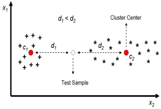
Figure 1.
Inefficiency of the distance to cluster’s center measure as a single criterion for choosing the proper cluster.
In the proposed approach, the large set of training data is first clustered using the K-means method similarly as it was done in [5]. These clusters may have different shapes and variant spread over axes. As it can be seen in Figure 1, considering this fact can affect the final classification results. To take into account the clusters spread over the axes, the following parameters are calculated for each cluster after the K-means process is finished:
where is the maximum Euclidean distance between data points of the cluster and it’s center () along the axis.
The idea is to define a metric which at least approximately shows the distance of a test data sample to a cluster border. To have more accurate approximate, this distance is calculated based on both the data point coordinates and the cluster’s spread on different axes as follows:
where is the approximate distance of the test sample from the cluster border, and is the Euclidean distance between the test sample and the center of the cluster (). Furthermore, the parameter indicates the number of dimensions in the data space.
Another factor which has an influence on choosing the proper cluster is its density. For example, between two clusters which their centers are at the same (or almost the same) distance from the test sample, the one with higher density will probably have better candidates to be the nearest neighbors for the test sample. Figure 2 shows two clusters with different densities. As it can be seen, for a 4-nn algorithm, for example, the four nearest neighbors can be found at closer distances by choosing cluster 2’s data as the training samples.
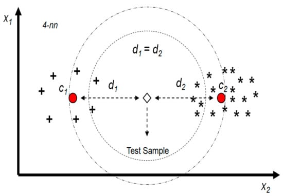
Figure 2.
The effect of cluster density on the KNN algorithm performance.
The density of a cluster is defined as follows:
where indicates the number of dimensions of the data space.
Based on these factors, the following Algorithms 1 and 2 are proposed for choosing a more proper cluster of data.
| Algorithm 1. Choosing the proper cluster. |
| Input: a test sample () to be classified by KNN and clusters of data |
| Output: a data cluster which is used for finding the nearest neighbors |
| 1. Begin |
| 2. for |
| 3. Find the Euclidean distance between and cluster center () |
| 4. end for |
| 5. for |
| 6. if |
| 7. return |
| 8. for each cluster which |
| 9. Calculate the distance defined by Equation (2) () |
| 10. for each cluster which |
| 11. if |
| 12. return |
| 13. for each cluster which |
| 14. Calculate the density of the cluster using Equation (3) () |
| 15. Choose the cluster with maximum density |
| 16. End |
The idea behind this algorithm is to take into account the distance to the clusters’ border metrics in the process of choosing the proper cluster when there is no considerable difference between the distances of the test sample from the clusters’ centers. As stated in lines 4–6, the cluster selection is the same as the base method if the center of one cluster (such as i) is significantly closer to the test sample in comparison to the other cluster’s center. However, if such a cluster does not exist, then the one in which the distance between its borders and the test sample is at a minimum is selected among the clusters with the closest centers (lines 9–11). When there is no significant difference between the distances to the clusters’ borders, the density of the clusters can play an effective role in choosing the proper cluster. The cluster with maximum density would be selected in this condition (line 14).
Finally, the proposed KNN algorithm for application on big data can be proposed based on Algorithm 1. First, the large amount of training data is clustered to m separate parts. After the clusters are determined, their size and their spread over different axes on the data space () should be calculated for each cluster. Employing Algorithm 1, the most proper cluster of data can be selected. Since the output of the KNN process depends on the training data used, selecting the best cluster of the data can have considerable effect on the final classification process. Consequently, the KNN algorithm is applied on the selected part of training data to finds the k nearest neighbors and, thus, to estimate the test sample’s class. The pseudocode of the proposed Algorithm 2 is shown below.
| Algorithm 2. The proposed KNN for big data. |
| Input: a large amount of data and a set of test samples that should be classified (data space has n dimension) |
| Output: the estimated class of each test sample |
| 1. Begin |
| 2. Divide the large amount of data to separate clusters using k-means algorithm |
| 3. For each cluster |
| 4. Calculate the size of cluster (number of data samples) |
| 5. Calculate |
| 6. For each test sample |
| 7. Choose the proper cluster of data by using Algorithm 1. |
| 8. Employ the KNN algorithm on the selected cluster to find the estimatedclass of the test sample |
| 9. End |
The performance of the proposed algorithm in comparison with some relevant recent studies is evaluated in the following section.
Parameters and represent the average distance between the test sample and the clusters’ centers and clusters’ borders, respectively. Furthermore, and are two tuning parameters (in the range of 0 to 1) which are suggested to be 0.5 and 0.7, respectively, based on experimental results. The higher value of the parameter means giving more importance to the distance to the clusters’ center metrics for choosing the proper cluster. In addition, the lower value of the parameters gives more importance to the density of clusters metric.
From a computational load point of view, the time complexity of the LC-KNN method is linear to the sample size, as stated in [5]. Since no loop of computation is added to the LC-KNN method and just two new cluster selection metrics are computed and employed by the proposed method, the time complexity of the proposed method is also linear to the sample size. The significant reduction in the size of the sample set which is explored for finding the nearest neighbors has led to the temporal superiority of the LC-KNN method and the proposed methods in comparison with the classic KNN one. It should be noted that the k-means clustering method is applied to the dataset only once, and the resulting clusters are used repeatedly for unseen samples. Furthermore, the metrics defined by Equations (1) and (3) are just calculated once for each cluster.
4. Experimental Results
As the proposed approach is an extension of the algorithm suggested in [5] (LC-KNN), its performance is compared with LC-KNN (as the baseline) on different real datasets [22,23,24,25,26,27]. The effect of some parameters’ value such as the number of clusters (m), number of neighbors (k), and on performance of the proposed approach has been also investigated in these experiments. The experimental results show the effectiveness of the proposed approach in comparison to the LC-KNN method. Before presenting and discussing the experimental results, the characteristics of the datasets used in the experiments are described in the following section.
4.1. The Characteristic of the Datasets
Nine datasets with different characteristics which are usually used in the previous related works are used for the evaluation. The number of instances and attributes which each dataset contains are stated in Table 1. An attempt was made to select different datasets from several fields with variant numbers of instances and attributes to have a more comprehensive and convincing evaluation.

Table 1.
The characteristics of the datasets.
4.2. Performance Evaluation with Different Values of the m Parameter
The value of the m parameter indicates the number of clusters which are the output of the k-means algorithm. As stated in [5], increasing the number of clusters usually leads to a decrease in classification accuracy. On the other hand, a higher value of the m parameter means breaking the vast amount of data into more clusters and, thus, spending less processing time for classification. However, when the number of clusters increases, choosing the proper cluster to search the neighbors in becomes more crucial. As the experiments show, the proposed approach selects the more appropriate cluster in comparison to LC-KNN method and, thus, shows better performance especially in the case of high numbers of cluster. Table 2 shows the classification accuracy of the proposed approach and LC-KNN on several datasets. The value of k, , and parameters are considered 1, 0.5, and 0.7, respectively, for this experiment.
Table 2.
Classification accuracy (mean of 10 runs) of the proposed approach and LC-KNN algorithm at different values of the m parameter.
As it can be seen, the proposed approach shows better classification accuracy almost in all situations. However, by decreasing the number of clusters (m parameter), the performance of the proposed approach becomes closer to LC-KNN.
4.3. The Effect of and Parameters’ Values on the Accuracy of the Proposed Method
Other factors that can have an effect on the performance are the values of and parameters. These parameters’ values are real numbers in the range of 0 to 1. Close to one value for the parameter makes the performance of the proposed approach and LC-KNN algorithm more similar, while smaller values for this parameter mean more usage of the distance to the boundary and the density criteria in the proper cluster selection process. Figure 3 shows the classification accuracy of the proposed approach for different values of the parameter on three different sample datasets. In these experiments, the value of the m, k, and parameters are considered 20, 1, and 0.7, respectively.
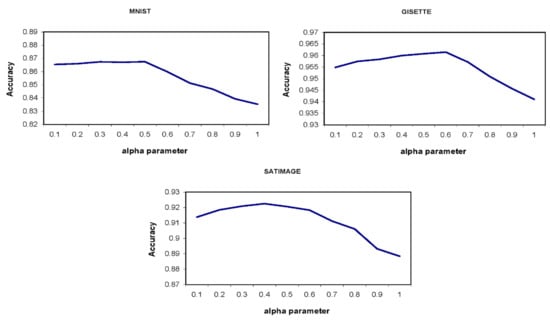
Figure 3.
Classification accuracy of the proposed approach for different values of the parameter. As it can be seen, the proposed approach has a better performance for the value of 0.5 on average.
As it can be seen, the optimal value for the parameter depends on the structure of the data; however, based on the results obtained from all experiments, the value of 0.5 is presented as a suggestion for this parameter. Similar experiments are conducted for investigating the effects of the value of the parameter on the proposed approach’s performance. Figure 4 shows the classification accuracy of the proposed approach for different values of the parameter. Higher value (near to 1) of the beta parameter means that most of the times the proper cluster is selected based on the distance from the clusters’ boundary. While lower values (near to zero) of this parameter mean taking the clusters’ density into account in the process of selecting the proper cluster more. The higher the value of the k parameter is, the grater the impact the clusters’ density may have on selecting the proper cluster; therefore, its value is considered 10 in this experiment. Furthermore, the value of the parameter is considered to be 0.5.
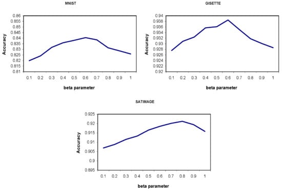
Figure 4.
Classification accuracy of the proposed approach for different values of the β parameter. As it can be seen, the proposed approach has a better performance for the value of 0.7 on average.
Based on all of the experiments done on different datasets, a value of 0.7 is suggested for the β parameter. Although the proposed approach shows better performance on average when 0.5 and 0.7 values are used for the and β parameters, it has also better classification accuracy in comparison to the LC-KNN approach even if other values in the range of (0,1) are used for these parameters.
Finally, the performance of the proposed approach (PA) is evaluated for different values of the k parameter. As the results show, the appropriate k value depends on the structural characteristics of the training dataset, such as the number of samples, density of the samples, each class’ sample frequency, etc. However, the overall classification accuracy decreases with the increase in the value of the k parameter. This reduction is much lower for the proposed approach because it takes the factors such as distance to the cluster’s border and the density of each cluster into account for the process of choosing the proper cluster. Figure 5 shows the experimental results over three different datasets. The value of m, , and parameters are considered 10, 0.5, and 0.7, respectively.
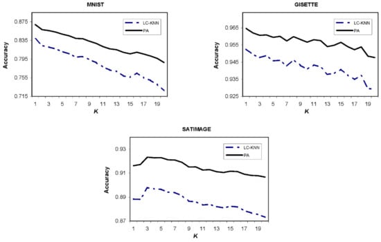
Figure 5.
Classification accuracy of the proposed approach (PA) and LC-KNN for different k values. As it can be seen, the higher values of the k parameter lead to the lower classification accuracy, in general, for both the proposed approach and LC-KNN.
4.4. Classification Accuracy and Time Cost Comparisons
In addition to LC-KNN, the performance of the proposed approach is compared with the original KNN and RFKNN methods in the classification accuracy and time cost points of view. In comparison with the original KNN, which is an exact method, helps to offer a better evaluation regarding the accuracy of the proposed method. On the other hand, RFKNN is an extension of the KNN for big data classification, which is the most related recent work to our proposed method, and also LC-KNN (as stated in Section 2). Table 3 shows the classification accuracy and time cost (in seconds) of these methods on the nine datasets. The experiments are repeated ten times, and the results are reported as the mean of these repetitions. It should be noted that the value of m, k, , and parameters are considered 20, 1, 0.5, and 0.7, respectively, in these experiments. Experiments are performed on a computer with 2.67 GHz CPU and 6 GB of RAM running Windows 7 as the operating system. In addition, all the methods are implemented and performed using the MATLAB (Massachusetts, USA) environment. During these experiments, all unnecessary OS services are disabled, and no concurrent program is run. As it can be seen, the proposed approach has better accuracy in comparison to the LC-KNN method and approximately the same accuracy in comparison with the RFKNN classifier. However, the proposed approach has lower computational complexity and, thus, time cost in comparison to the RFKNN classifier. This higher execution time is due to the fact that the RFKNN classifier usually searches for the nearest neighbors of a test sample in a larger dataset than of the one searched in the proposed approach. Obviously, the original KNN method can achieve better accuracy at the cost of greater execution time.
Table 3.
Classification accuracy and time cost of the proposed approach in comparison to the other related works on different datasets.
5. Conclusions
With increases in databases’ volumes, traditional machine learning methods almost cannot be performed by a single processing machine in an acceptable time anymore. Therefore, two main approaches have been proposed by researchers to address this problem: using high-performance computing systems or reducing the amount of required computation. This paper has focused on devising an efficient KNN classification algorithm for big data. The proposed classifier initially partitions the large amount of training data into smaller subsets by using a clustering algorithm, such as k-means, and then applies the KNN method for each new unseen sample on the cluster with the nearest center for the classification phase. It has been shown and discussed with some examples, in the proposed approach section, that the minimum distance between the cluster’s center and the test sample alone is not an efficient criterion. The shape and density of the clusters are also two important factors that have significant impacts on choosing the proper cluster and, thus, classification accuracy. Two parameters have been defined in order to consider these two factors in choosing the proper cluster and, thus, reducing the data volume more intelligently. Experimental results show that the proposed approach has better classification accuracy in comparison to other recent relevant methods. It has also been shown that the proposed method has a shorter execution time in comparison to the RFKNN method.
Author Contributions
Methodology: H.S., S.K., J.H.J., and A.M.; software: H.S., S.K., J.H.J., and, A.M.; validation: H.S., S.K., J.H.J., and A.M.; formal analysis: H.S., S.K., J.H.J., and A.M.; investigation: H.S., S.K., J.H.J., and A.M.; resources: H.S., S.K., J.H.J., and A.M.; data curation: H.S., S.K., J.H.J., and A.M.; writing—original draft preparation: H.S., S.K., J.H.J., and A.M.; writing—review and editing: H.S., S.K., J.H.J., and A.M.; visualization: H.S., S.K., J.H.J., and A.M.; supervision: S.S.; project administration and research submission: S.S.; funding acquisition: A.M. All authors have read and agreed to the published version of the manuscript.
Funding
We acknowledge the financial support of this work by the Hungarian State and the European Union under the EFOP-3.6.1-16-2016-00010 project and the 2017-1.3.1-VKE-2017-00025 project.
Acknowledgments
We acknowledge the support of the German Research Foundation (DFG) and the Bauhaus-Universität Weimar within the Open-Access Publishing Programme.
Conflicts of Interest
The authors declare no conflict of interest.
References
- Wu, X.; Zhu, X.; Wu, G.Q.; Ding, W. Data mining with big data. IEEE Trans. Knowl. Data Eng. 2014, 26, 97–107. [Google Scholar]
- Anchalia, P.P.; Roy, K. The k-Nearest Neighbor Algorithm Using MapReduce Paradigm. In Proceedings of the 2014 5th International Conference on Intelligent Systems, Modelling and Simulation, Langkawi, Malaysia, 27–29 January 2014; pp. 513–518. [Google Scholar]
- Neeb, H.; Kurrus, C. Distributed K-Nearest Neighbors; Stanford University Publishing: Stanford, CA, USA, 2016. [Google Scholar]
- Yong, Z.; Youwen, L.; Shixiong, X. An improved KNN text classification algorithm based on clustering. J. Comput. 2009, 4, 230–237. [Google Scholar]
- Deng, Z.; Zhu, X.; Cheng, D.; Zong, M.; Zhang, S. Efficient kNN classification algorithm for big data. Neurocomputing 2016, 195, 143–148. [Google Scholar] [CrossRef]
- Wu, X.; Kumar, V.; Quinlan, J.R.; Ghosh, J.; Yang, Q.; Motoda, H.; Philip, S.Y. Top 10 algorithms in data mining. Knowl. Inf. Syst. 2008, 14, 1–37. [Google Scholar] [CrossRef]
- Zhang, C.; Li, F.; Jestes, J. Efficient parallel kNN joins for large data in MapReduce. In Proceedings of the 15th International Conference on Extending Database Technology, Berlin, Germany, 26–30 March 2012; pp. 38–49. [Google Scholar]
- Sun, K.; Kang, H.; Park, H.-H. Tagging and classifying facial images in cloud environments based on KNN using MapReduce. Opt. Int. J. Light Electron Opt. 2015, 126, 3227–3233. [Google Scholar] [CrossRef]
- Chatzigeorgakidis, G.; Karagiorgou, S.; Athanasiou, S.; Skiadopoulos, S. FML-kNN: Scalable machine learning on Big Data using k-nearest neighbor joins. J. Big Data 2018, 5, 4. [Google Scholar] [CrossRef]
- Plaku, E.; Kavraki, L.E. Distributed Computation of the knn Graph for Large High-Dimensional Point Sets. J. Parallel Distrib. Comput. 2007, 67, 346–359. [Google Scholar] [CrossRef]
- Kim, W.; Kim, Y.; Shim, K. Parallel computation of k-nearest neighbor joins using MapReduce. In Proceedings of the 2016 IEEE International Conference on Big Data, Washington, DC, USA, 5–8 December 2016; pp. 696–705. [Google Scholar]
- Garcia, V.; Debreuve, E.; Barlaud, M. Fast k Nearest Neighbor Search using GPU. In Proceedings of the 2008 IEEE Computer Society Conference on Computer Vision and Pattern Recognition Workshops, Anchorage, AK, USA, 23–28 June 2008; pp. 1–6. [Google Scholar]
- Garcia, V.; Debreuve, E.; Nielsen, F.; Barlaud, M. K-nearest neighbor Search: Fast gpu-based implementations and application to high-dimensional feature matching. In Proceedings of the 2010 IEEE International Conference on Image Processing, Hong Kong, China, 12–15 September 2010; pp. 3757–3760. [Google Scholar]
- Lu, W.; Shen, Y.; Chen, S.; Chin Ooi, B. Efficient Processing of k Nearest Neighbor Joins using MapReduce. Proc. VLDB Endow. 2012, 5, 1016–1027. [Google Scholar] [CrossRef]
- Connor, M.; Piyush, K. Fast construction of k-nearest neighbor graphs for point clouds. IEEE Trans. Vis. Comput. Gr. 2010, 16, 599–608. [Google Scholar] [CrossRef] [PubMed]
- Valero-Mas, J.J.; Calvo-Zaragoza, J.; Rico-Juan, J.R. On the suitability of Prototype Selection methods for kNN classification with distributed data. Neurocomputing 2016, 203, 150–160. [Google Scholar] [CrossRef]
- Angiulli, F. Fast condensed nearest neighbor rule. In Proceedings of the 22nd International Conference on Machine Learning, Bonn, Germany, 7–11 August 2005; pp. 25–32. [Google Scholar]
- Seidl, T.; Kriegel, H.-P. Optimal multi-step k-nearest neighbor search. ACM SIGMOD Rec. 1998, 27, 154–165. [Google Scholar] [CrossRef]
- Li, R.-L.; Hu, Y. A density-based method for reducing the amount of training data in kNN text classification. J. Comput. Res. Dev. 2004, 41, 539–545. [Google Scholar]
- Chen, Y.; Hu, X.; Fan, W.; Shen, L.; Zhang, Z.; Liu, X.; Li, H. Fast density peak clustering for large scale data based on kNN. Knowl. Based Syst. 2020, 187, 104824. [Google Scholar] [CrossRef]
- Mahfouz, M. Rfknn: Rough-Fuzzy Knn for Big Data Classification. Int. J. Adv. Res. Comput. Sci. 2018, 9, 274. [Google Scholar] [CrossRef]
- Chang, C.-C.; Lin, C.-J. LIBSVM: A library for support vector machines. ACM Trans. Intell. Syst. Technol. 2011, 2, 1–27. [Google Scholar] [CrossRef]
- Gao, Y.; Wang, M.; Zha, Z.J.; Shen, J.; Li, X.; Wu, X. Visual-textual joint relevance learning for tag-based social image search. IEEE Trans. Image Process. 2013, 22, 363–376. [Google Scholar] [CrossRef] [PubMed]
- Gao, Y.; Wang, M.; Tao, D.; Ji, R.; Dai, Q. 3-D object retrieval and recognition with hypergraph analysis. IEEE Trans. Image Process. 2012, 21, 4290–4303. [Google Scholar] [CrossRef] [PubMed]
- Liu, W.; Zhang, H.; Tao, D.; Wang, Y.; Lu, K. Large-scale paralleled sparse principal component analysis. Multimed. Tools Appl. 2016, 75, 1481–1493. [Google Scholar] [CrossRef]
- Bache, K.; Lichman, M. UCI Machine Learning Repository 2013. University of California, School of Information and Computer Science. Available online: http://archive.ics.uci.edu/ml (accessed on 26 November 2019).
- Shabani, S.; Samadianfard, S.; Sattari, M.T.; Mosavi, A.; Shamshirband, S.; Kmet, T.; Várkonyi-Kóczy, A.R. Modeling Pan Evaporation Using Gaussian Process Regression K-Nearest Neighbors Random Forest and Support Vector Machines; Comparative Analysis. Atmosphere 2020, 11, 66. [Google Scholar] [CrossRef]
© 2020 by the authors. Licensee MDPI, Basel, Switzerland. This article is an open access article distributed under the terms and conditions of the Creative Commons Attribution (CC BY) license (http://creativecommons.org/licenses/by/4.0/).