Alternating Asymmetric Iterative Algorithm Based on Domain Decomposition for 3D Poisson Problem

Abstract

Poisson equation is a widely used partial differential equation. It is very important to study its numerical solution. Based on the strategy of domain decomposition, the alternating asymmetric iterative algorithm for 3D Poisson equation is provided. The solution domain is divided into several sub-domains, and eight asymmetric iterative schemes with the relaxation factor for 3D Poisson equation are constructed. When the numbers of iteration are odd or even, the computational process of the presented iterative algorithm are proposed respectively. In the calculation of the inner interfaces, the group explicit method is used, which makes the algorithm to be performed fast and in parallel, and avoids the difficulty of solving large-scale linear equations. Furthermore, the convergence of the algorithm is analyzed theoretically. Finally, by comparing with the numerical experimental results of Jacobi and Gauss Seidel iterative algorithms, it is shown that the alternating asymmetric iterative algorithm based on domain decomposition has shorter computation time, fewer iteration numbers and good parallelism.

1. Introduction

Poisson equation is an elliptic partial differential equation, which frequently appears in many fields such as fluid dynamics, heat transfer, electromagnetics, acoustics, electrostatics mechanical engineering and so on. Many researches on studding the numerical techniques to approximate the solution of Poisson equation have been made in the past few decades. The application of finite difference methods for solving Poisson equation will normally lead to a large, block, and sparse system of equations. Direct methods and iterative methods [1] are normally considered as common approaches for solving such system of equations. Several high precision multigrid and compact difference methods are given in [2,3,4,5,6]. Romao et al. [7,8] provides the Galerkin and least-squares finite element methods in the solution of 3D Poisson equation. In [9,10], the Haar wavelet methods are given. Speyer et al. [11] provide a preconditioned bi-conjugate gradient stabilized method which is efficient, albeit nonmonotonic and convergent.

With the continuous improvement of computer hardware, people are more and more focused on solving large-scale scientific and engineering problems quickly and efficiently on parallel computers. Therefore, people wish to find some direct methods and iterative methods, which have the characteristic of much better solving elliptic equations and easier parallel implementation. In recent years, parallel algorithms are also constantly emerging. Several new parallel methods of direct solution are proposed. P. Valero-Lara and A. Pinelli et al. [12] provide the implementation of a fast solver based on a block cyclic reduction algorithm for the linear systems of a three dimensional separable elliptic problem. And they also study on the parallel characteristics of an algorithm for the direct solution of linear systems with a block-tridiagonal coefficient matrix (BLKTRI problem) [13]. C. P. Stone et al. [14] analyze the performance of a block tridiagonal benchmark. Many authors have given the implementation of scalar tridiagonal solver on GPUs [15,16,17]. Y. Zhang [16] also illustrates several methods to solve tridiagonal systems on GPUs. Because of the direct method to solve large-scale sparse and block diagonal equation systems, when the coefficient matrix is close to singularity, the calculation will often stop or make mistakes. So people also find iterative methods which can be solved by constructing some efficient iterative schemes to approximate the problem itself, so that the iteration can reach a certain accuracy. In [18,19,20,21], a class of efficient parallel finite difference iterative algorithms for Poisson equation were also proposed.

In addition, the domain decomposition method [22] is also a powerful tool for parallel implementation, which studies parallelization from the model level of physical problems. This kind of method can decompose scale problem into small-scale problem and solve serial problem into parallel problem. The explicit-implicit domain decomposition method is proposed by Kuznetsov [23]. Because the numerical boundary conditions on the internal boundary are often not the same as those of the original mathematical model or the corresponding physical problems, different methods to obtain the internal boundary information form different explicit-implicit domain decomposition (EIDD) methods. This leads to the idea of parallel implementation for iterative method based on domain decomposition. In [24], the authors have proposed a kind of finite difference parallel iterative algorithm for two-dimensional Poisson problem, and verified its efficiency and accuracy.

This paper extends to the study of the domain decomposition method for three-dimensional Poisson problem. Several finite difference asymmetric iterative schemes are constructed, and each asymmetric iterative schemes are used to solve the sub-domains alternatively and in parallel; in the processing of inner interfaces, group explicit (GE) method [25,26] is used. The calculation on the whole solution domain is explicit but using the implicit iterative schemes, which greatly avoids the difficulty of solving linear equations and improves the calculation speed and accuracy. When the number of iteration is odd or even, the iterative process of the presented algorithm is given respectively, and a kind of efficient iterative algorithm is established based on domain decomposition for solving three-dimensional Poisson equation.

This paper is outlined as follows. In Section 2, we present several asymmetric iterative schemes. Section 3 gives the alternating asymmetric iterative algorithm. And the convergence and the optimal relaxation factor are obtained in Section 4. In Section 5, we perform the numerical experiments to examine the presented algorithm. Finally we give the conclusion of this paper in Section 6.

2. Asymmetric Iterative Schemes

Consider the three-dimensional Poisson problem,

$$\frac{{\partial }^{2}u}{\partial x^2}+\frac{{\partial }^{2}u}{\partial y^2}+\frac{{\partial }^{2}u}{\partial z^2}=f(x,y,z),(x,y,z)\in \mathsf{\Omega },$$

(1)

with the boundary condition,

$$u(x,y,z)=g(x,y,z),(x,y,z)\in \partial \mathsf{\Omega }.$$

(2)

where $\mathsf{\Omega }=[0,L]\times [0,M]\times [0,K]$, and $\partial \mathsf{\Omega }$ is the boundary of the domain $\mathsf{\Omega }$. We divide the solution domain $\mathsf{\Omega }$ into uniform grid, the space step $h_x=L/l$ in x direction, $h_y=M/m$ in y direction and $h_z=K/s$ in z direction. For implicity, the space steps are assumed equal that $h_x=h_y=h_z=h$. Denote $x_i=ih,i=0,1,\dots ,l$; $y_j=jh,j=0,1,\dots ,m$; $z_k=kh,k=0,1,\dots ,s$; $u_{i,j,k}^{\left(n\right)}$ as numerical solution on the nth iteration level at the grid node $(x_i,y_j,z_k)$. We can give the classical difference discretization in Equation (3) for the 3D Poisson Equation (1),

$$\frac{u_{i+1,j,k}-2u_{i,j,k}+u_{i-1,j,k}}{h^2}+\frac{u_{i,j+1,k}-2u_{i,j,k}+u_{i,j-1,k}}{h^2}+\frac{u_{i,j,k+1}-2u_{i,j,k}+u_{i,j,k-1}}{h^2}=f_{i,j,k},$$

(3)

namely,

$$u_{i,j,k}-\frac{1}{6}(u_{i+1,j,k}+u_{i-1,j,k}+u_{i,j+1,k}+u_{i,j-1,k}+u_{i,j,k+1}+u_{i,j,k-1}-h^2{f}_{i,j,k})=0.$$

(4)

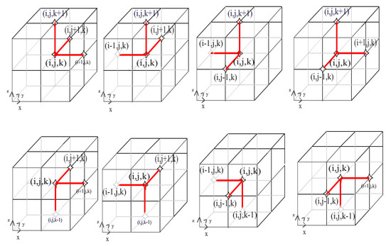
Then we construct eight asymmetric iterative schemes by the difference operator L with the relaxation factor $\omega$ as follows,

$$\begin{array}{cc}\hfill L_1{u}_{i,j,k}^{(n+1)}=u_{i,j,k}^{(n+1)}-\frac{1}{6}\left[\omega (u_{i+1,j,k}^{(n+1)}\right.& +u_{i,j+1,k}^{(n+1)}+u_{i,j,k+1}^{(n+1)})+u_{i-1,j,k}^{\left(n\right)}+u_{i,j-1,k}^{\left(n\right)}+u_{i,j,k-1}^{\left(n\right)}\hfill \\ & \left.+(1-\omega )(u_{i+1,j,k}^{\left(n\right)}+u_{i,j+1,k}^{\left(n\right)}+u_{i,j,k+1}^{\left(n\right)})-h^2{f}_{i,j,k}\right],\hfill \end{array}$$

(5)

$$\begin{array}{cc}\hfill L_2{u}_{i,j,k}^{(n+1)}=u_{i,j,k}^{(n+1)}-\frac{1}{6}\left[\omega (u_{i-1,j,k}^{(n+1)}\right.& +u_{i,j+1,k}^{(n+1)}+u_{i,j,k+1}^{(n+1)})+u_{i+1,j,k}^{\left(n\right)}+u_{i,j-1,k}^{\left(n\right)}+u_{i,j,k-1}^{\left(n\right)}\hfill \\ & \left.+(1-\omega )(u_{i-1,j,k}^{\left(n\right)}+u_{i,j+1,k}^{\left(n\right)}+u_{i,j,k+1}^{\left(n\right)})-h^2{f}_{i,j,k}\right],\hfill \end{array}$$

(6)

$$\begin{array}{cc}\hfill L_3{u}_{i,j,k}^{(n+1)}=u_{i,j,k}^{(n+1)}-\frac{1}{6}\left[\omega (u_{i-1,j,k}^{(n+1)}\right.& +u_{i,j-1,k}^{(n+1)}+u_{i,j,k+1}^{(n+1)})+u_{i+1,j,k}^{\left(n\right)}+u_{i,j+1,k}^{\left(n\right)}+u_{i,j,k-1}^{\left(n\right)}\hfill \\ & \left.+(1-\omega )(u_{i-1,j,k}^{\left(n\right)}+u_{i,j-1,k}^{\left(n\right)}+u_{i,j,k+1}^{\left(n\right)})-h^2{f}_{i,j,k}\right],\hfill \end{array}$$

(7)

$$\begin{array}{cc}\hfill L_4{u}_{i,j,k}^{(n+1)}=u_{i,j,k}^{(n+1)}-\frac{1}{6}\left[\omega (u_{i+1,j,k}^{(n+1)}\right.& +u_{i,j-1,k}^{(n+1)}+u_{i,j,k+1}^{(n+1)})+u_{i-1,j,k}^{\left(n\right)}+u_{i,j+1,k}^{\left(n\right)}+u_{i,j,k-1}^{\left(n\right)}\hfill \\ & \left.+(1-\omega )(u_{i+1,j,k}^{\left(n\right)}+u_{i,j-1,k}^{\left(n\right)}+u_{i,j,k+1}^{\left(n\right)})-h^2{f}_{i,j,k}\right],\hfill \end{array}$$

(8)

$$\begin{array}{cc}\hfill L_5{u}_{i,j,k}^{(n+1)}=u_{i,j,k}^{(n+1)}-\frac{1}{6}\left[\omega (u_{i+1,j,k}^{(n+1)}\right.& +u_{i,j+1,k}^{(n+1)}+u_{i,j,k-1}^{(n+1)})+u_{i-1,j,k}^{\left(n\right)}+u_{i,j-1,k}^{\left(n\right)}+u_{i,j,k+1}^{\left(n\right)}\hfill \\ & \left.+(1-\omega )(u_{i+1,j,k}^{\left(n\right)}+u_{i,j+1,k}^{\left(n\right)}+u_{i,j,k-1}^{\left(n\right)})-h^2{f}_{i,j,k}\right],\hfill \end{array}$$

(9)

$$\begin{array}{cc}\hfill L_6{u}_{i,j,k}^{(n+1)}=u_{i,j,k}^{(n+1)}-\frac{1}{6}\left[\omega (u_{i-1,j,k}^{(n+1)}\right.& +u_{i,j+1,k}^{(n+1)}+u_{i,j,k-1}^{(n+1)})+u_{i+1,j,k}^{\left(n\right)}+u_{i,j-1,k}^{\left(n\right)}+u_{i,j,k+1}^{\left(n\right)}\hfill \\ & \left.+(1-\omega )(u_{i-1,j,k}^{\left(n\right)}+u_{i,j+1,k}^{\left(n\right)}+u_{i,j,k-1}^{\left(n\right)})-h^2{f}_{i,j,k}\right],\hfill \end{array}$$

(10)

$$\begin{array}{cc}\hfill L_7{u}_{i,j,k}^{(n+1)}=u_{i,j,k}^{(n+1)}-\frac{1}{6}\left[\omega (u_{i-1,j,k}^{(n+1)}\right.& +u_{i,j-1,k}^{(n+1)}+u_{i,j,k-1}^{(n+1)})+u_{i+1,j,k}^{\left(n\right)}+u_{i,j+1,k}^{\left(n\right)}+u_{i,j,k+1}^{\left(n\right)}\hfill \\ & \left.+(1-\omega )(u_{i-1,j,k}^{\left(n\right)}+u_{i,j-1,k}^{\left(n\right)}+u_{i,j,k-1}^{\left(n\right)})-h^2{f}_{i,j,k}\right],\hfill \end{array}$$

(11)

$$\begin{array}{cc}\hfill L_8{u}_{i,j,k}^{(n+1)}=u_{i,j,k}^{(n+1)}-\frac{1}{6}\left[\omega (u_{i+1,j,k}^{(n+1)}\right.& +u_{i,j-1,k}^{(n+1)}+u_{i,j,k-1}^{(n+1)})+u_{i-1,j,k}^{\left(n\right)}+u_{i,j+1,k}^{\left(n\right)}+u_{i,j,k+1}^{\left(n\right)}\hfill \\ & \left.+(1-\omega )(u_{i+1,j,k}^{\left(n\right)}+u_{i,j-1,k}^{\left(n\right)}+u_{i,j,k-1}^{\left(n\right)})-h^2{f}_{i,j,k}\right],\hfill \end{array}$$

(12)

Figure 1 represents the distribution of unknown solution at the $(n+1)$th iteration level for the eight asymmetric iterative schemes (5)–(12).

Figure 1. The asymmetric iterative schemes (5)–(12) for the 3D Poisson equation with the relaxation factor $\omega$.

3. Alternating Asymmetric Iterative Algorithm Based on Domain Decomposition

3.1. The Domain Decomposition

We can divide the 3D solution domain $\mathsf{\Omega }$ into multi-subdomains. For simplicity, we use six grid planes $x=p,x=p+1,y=q,y=q+1,z=r,z=r+1$ to discrete the solution domain $\mathsf{\Omega }$ into eight sub-domains, and note ${\mathsf{\Omega }}_i,i=1,2,\dots ,8$ as subsets of grid points, while $p,q,r$ are positive integers with $p\in [1,l],q\in [1,m],r\in [1,s]$. Denote ${\pi }_i$ is the interfaces of the sub-domain ${\mathsf{\Omega }}_i$. The sorting order of sub-domains is as follows: the subspaces above $z=r+1$ are sorted anticlockwise starting from the upper right sub-domain of the inner layer, and the sub-domains under $z=r$ are sorted anticlockwise starting from the lower right subspace (as shown in Figure 2). The specific description is as follows:

$$\begin{array}{cc}{\mathsf{\Omega }}_1:& \left\{(x,y,z)|x=l-1,l-2,\dots ,p+1;y=m-1,m-2,\dots ,q+1;z=s-1,s-2,\dots ,r+1\right\},\hfill \\ {\mathsf{\Omega }}_2:& \left\{(x,y,z)|x=1,2,\dots ,p;y=m-1,m-2,\dots ,q+1;z=s-1,s-2,\dots ,r+1\right\},\hfill \\ {\mathsf{\Omega }}_3:& \left\{(x,y,z)|x=1,2,\dots ,p;y=1,2,\dots ,q;z=s-1,s-2,\dots ,r+1\right\},\hfill \\ {\mathsf{\Omega }}_4:& \left\{(x,y,z)|x=l-1,l-2,\dots ,p+1;y=1,2,\dots ,q;z=s-1,s-2,\dots ,r+1\right\},\hfill \\ {\mathsf{\Omega }}_5:& \left\{(x,y,z)|x=l-1,l-2,\dots ,p+1;y=m-1,m-2,\dots ,q+1;z=1,2,\dots ,r\right\},\hfill \\ {\mathsf{\Omega }}_6:& \left\{(x,y,z)|x=1,2,\dots ,p;y=m-1,m-2,\dots ,q+1;z=1,2,\dots ,r\right\},\hfill \\ {\mathsf{\Omega }}_7:& \left\{(x,y,z)|x=1,2,\dots ,p;y=1,2,\dots ,q;z=1,2,\dots ,r\right\},\hfill \\ {\mathsf{\Omega }}_8:& \left\{(x,y,z)|x=l-1,l-2,\dots ,p+1;y=1,2,\dots ,q;z=1,2,\dots ,r\right\}.\hfill \end{array}$$

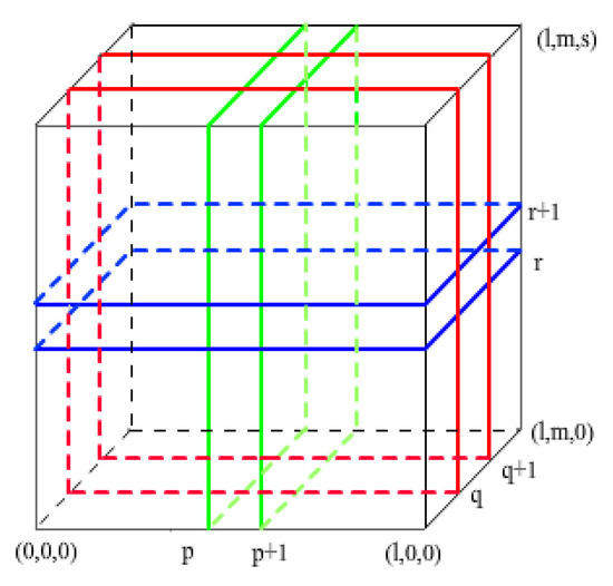
Figure 2. The solution domain is divided into eight sub-domains.

3.2. Algorithm Implementation

In this subsection, we provide a new alternating asymmetric iterative (AAI) algorithm based on domain decomposition for 3D Poisson problem (1) and (2). We give different computational processes in each sub-domains at the odd iteration layers and even iteration layers respectively, and use the asymmetric iterative schemes alternatively. The Group Explicit (GE) method is used to solve the inner interfaces, which makes the algorithm to be computed fast and in parallel, and avoids the difficulty of solving large-scale linear equations.

3.2.1. Implementation of Odd Level Iteration

When the iteration number are odd, namely, $n=2a+1,a=0,1,\dots$, we solve the grid nodes from the boundaries to the inner interfaces step by step, that is, using the asymmetric iterative schemes (5)–(12) to solve the grid points in ${\mathsf{\Omega }}_i,i=1,2,\dots ,8$ respectively:

$$\left\{\begin{array}{cc}{L}_1{u}_{i,j,k}^{(2a+1)}=0,& (i,j,k)\in {\mathsf{\Omega }}_1,\\ L_2{u}_{i,j,k}^{(2a+1)}=0,& (i,j,k)\in {\mathsf{\Omega }}_2,\\ L_3{u}_{i,j,k}^{(2a+1)}=0,& (i,j,k)\in {\mathsf{\Omega }}_3,\\ L_4{u}_{i,j,k}^{(2a+1)}=0,& (i,j,k)\in {\mathsf{\Omega }}_4,\\ L_5{u}_{i,j,k}^{(2a+1)}=0,& (i,j,k)\in {\mathsf{\Omega }}_5,\\ L_6{u}_{i,j,k}^{(2a+1)}=0,& (i,j,k)\in {\mathsf{\Omega }}_6,\\ L_7{u}_{i,j,k}^{(2a+1)}=0,& (i,j,k)\in {\mathsf{\Omega }}_7,\\ L_8{u}_{i,j,k}^{(2a+1)}=0,& (i,j,k)\in {\mathsf{\Omega }}_8.\end{array}\right.$$

(13)

Obviously, the numerical solution can be obtained independently in parallel when the iteration numbers are odd, which saves a lot of computational time compared with the full-implicit iteration case. In addition, although the asymmetric iterative schemes are implicit, the computational process can be transformed into explicit, which can obviously improve the calculation speed and avoid solving large and complex linear equations.

3.2.2. Implementation of Even Level Iteration

When the iteration number is even, namely, $n=2a+2,a=0,1,\dots$, we calculate the numerical solution from the inner interfaces to the boundaries step by step. Where the computational process of the interfaces $\pi =\bigcup {\pi }_i,i=1,2,\dots ,8$ includes three parts:

• Interfaces I (namely, the grid nodes at the center of the domain $\mathsf{\Omega }$) (shown in Figure 3): $(p,q,r+1),(p+1,q,r+1),(p+1,q+1,r+1),(p,q+1,r+1),(p,q,r),(p+1,q,r),(p+1,q+1,r),(p,q+1,r)$.
  

  Figure 3. The computation of the interfaces $I,II,III$.
• Interfaces II: the interface lines except Interfaces I (shown in Figure 3).
• Interfaces III: the interfaces except Interfaces I and II, namely,
  $\pi \backslash InterfacesI\cup InterfacesII$.

Therefore, it can be seen that the interfaces $\pi =$ Interfaces I ∪ Interfaces II ∪ Interfaces III. When the interfaces $\pi$ are solved, the inner grid nodes in the domain $\mathsf{\Omega }$ can be solved in order like the odd case of iteration numbers in Section 3.2.1. We give the computational procedures in detail as follows.

(1) The solution to Interfaces I

We use the asymmetric iterative schemes (5)–(12) to solve the Interfaces I, then the following linear equations can be obtained:

$$M_1\left[\begin{array}{c}{u}_{p+1,q+1,r+1}^{(2a+2)}\\ u_{p,q+1,r+1}^{(2a+2)}\\ u_{p,q,r+1}^{(2a+2)}\\ u_{p+1,q,r+1}^{(2a+2)}\\ u_{p+1,q+1,r}^{(2a+2)}\\ u_{p,q+1,r}^{(2a+2)}\\ u_{p,q,r}^{(2a+2)}\\ u_{p+1,q,r}^{(2a+2)}\end{array}\right]=N_1,$$

(14)

where matrices $M_1$ and $N_1$ are represented as bellow,

$$M_1=\left[\begin{array}{cccccccc}6& -\omega & & -\omega & -\omega & & & \\ -\omega & 6& -\omega & & & -\omega & & \\ & -\omega & 6& -\omega & & & -\omega & \\ -\omega & & -\omega & 6& & & & -\omega \\ -\omega & & & & 6& -\omega & & -\omega \\ & -\omega & & & -\omega & 6& -\omega & \\ & & -\omega & & & -\omega & 6& -\omega \\ & & & -\omega & -\omega & & -\omega & 6\end{array}\right],N_1=\left[\begin{array}{c}{e}_1\\ e_2\\ e_3\\ e_4\\ e_5\\ e_6\\ e_7\\ e_8\end{array}\right],$$

$$\begin{array}{ccc}\hfill e_1& =& u_{p+2,q+1,r+1}^{(2a+1)}+u_{p+1,q+2,r+1}^{(2a+1)}+u_{p+1,q+1,r+2}^{(2a+1)}+(1-\omega )(u_{p,q+1,r+1}^{(2a+1)}+u_{p+1,q,r+1}^{(2a+1)}\hfill \\ & & +u_{p+1,q+1,r}^{(2a+1)})-h^2{f}_{p+1,q+1,r+1},\hfill \\ \hfill e_2& =& u_{p-1,q+1,r+1}^{(2a+1)}+u_{p,q+2,r+1}^{(2a+1)}+u_{p,q+1,r+2}^{(2a+1)}+(1-\omega )(u_{p+1,q+1,r+1}^{(2a+1)}+u_{p,q,r+1}^{(2a+1)}+u_{p,q+1,r}^{(2a+1)})\hfill \\ & & -h^2{f}_{p,q+1,r+1},\hfill \\ \hfill e_3& =& u_{p-1,q,r+1}^{(2a+1)}+u_{p,q-1,r+1}^{(2a+1)}+u_{p,q,r+2}^{(2a+1)}+(1-\omega )(u_{p+1,q,r+1}^{(2a+1)}+u_{p,q+1,r+1}^{(2a+1)}+u_{p,q,r}^{(2a+1)})\hfill \\ & & -h^2{f}_{p,q,r+1},\hfill \\ \hfill e_4& =& u_{p+2,q,r+1}^{(2a+1)}+u_{p+1,q-1,r+1}^{(2a+1)}+u_{p+1,q,r+2}^{(2a+1)}+(1-\omega )(u_{p,q,r+1}^{(2a+1)}+u_{p+1,q+1,r+1}^{(2a+1)}+u_{p+1,q,r}^{(2a+1)})\hfill \\ & & -h^2{f}_{p+1,q,r+1},\hfill \\ \hfill e_5& =& u_{p+2,q+1,r}^{(2a+1)}+u_{p+1,q+2,r}^{(2a+1)}+u_{p+1,q+1,r-1}^{(2a+1)}+(1-\omega )(u_{p,q+1,r}^{(2a+1)}+u_{p+1,q,r}^{(2a+1)}+u_{p+1,q+1,r+1}^{(2a+1)})\hfill \\ & & -h^2{f}_{p+1,q+1,r},\hfill \\ \hfill e_6& =& u_{p-1,q+1,r}^{(2a+1)}+u_{p,q+2,r}^{(2a+1)}+u_{p,q+1,r-1}^{(2a+1)}+(1-\omega )(u_{p+1,q+1,r}^{(2a+1)}+u_{p,q,r}^{(2a+1)}+u_{p,q+1,r+1}^{(2a+1)})\hfill \\ & & -h^2{f}_{p,q+1,r},\hfill \\ \hfill e_7& =& u_{p-1,q,r}^{(2a+1)}+u_{p,q-1,r}^{(2a+1)}+u_{p,q,r-1}^{(2a+1)}+(1-\omega )(u_{p+1,q,r}^{(2a+1)}+u_{p,q+1,r}^{(2a+1)}+u_{p,q,r+1}^{(2a+1)})\hfill \\ & & -h^2{f}_{p,q,r},\hfill \\ \hfill e_8& =& u_{p+2,q,r}^{(2a+1)}+u_{p+1,q-1,r}^{(2a+1)}+u_{p+1,q,r-1}^{(2a+1)}+(1-\omega )(u_{p,q,r}^{(2a+1)}+u_{p+1,q+1,r}^{(2a+1)}+u_{p+1,q,r+1}^{(2a+1)})\hfill \\ & & -h^2{f}_{p+1,q,r}.\hfill \end{array}$$

Then we just solve the above eight-order sparse linear Equation (14) to obtain the numerical solution of the $interfaceI$.

(2) The solution to Interfaces II

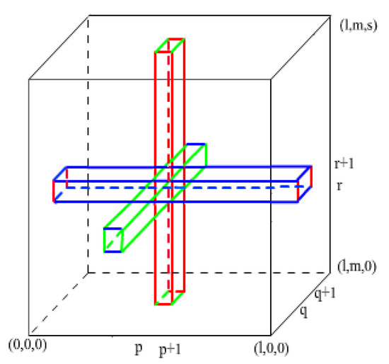
The computational procedure of the Interfaces I is depending on the use of GE method based on eight points per group. Similarly, we use the GE method based on four points per group to solve the Interfaces II between the inner boundaries of eight subspaces ${\mathsf{\Omega }}_i,i=1,2,\dots ,8$. Take one group of the Interfaces II for example to illustrate the order of the solution process. Figure 3 gives the direction of the iteration computation.

Using the asymmetric iterative schemes (6), (7), (10), (11) to solve the grid nodes $(i,q,r),(i,q,r+1),(i,q+1,r+1),(i,q+1,r)i=p+2,p+3,\dots ,l-1$ (shown in Figure 3), then we can provide the following fourth-order linear equations:

$$\left[\begin{array}{cccc}6& -\omega & & -\omega \\ -\omega & 6& -\omega \\ & -\omega & 6& -\omega \\ -\omega & & -\omega & 6\end{array}\right]\left[\begin{array}{c}{u}_{i,q,r}^{(2a+2)}\\ u_{i,q,r+1}^{(2a+2)}\\ u_{i,q+1,r+1}^{(2a+2)}\\ u_{i,q+1,r}^{(2a+2)}\end{array}\right]=\left[\begin{array}{c}{d}_1\\ d_2\\ d_3\\ d_4\end{array}\right],$$

(15)

where

$$\begin{array}{cc}{d}_1=\hfill & \omega u_{i-1,q,r}^{(2a+2)}+u_{i+1,q,r}^{(2a+1)}+u_{i,q-1,r}^{(2a+1)}+u_{i,q,r-1}^{(2a+1)}+(1-\omega )(u_{i-1,q,r}^{(2a+1)}+u_{i,q+1,r}^{(2a+1)}+u_{i,q,r+1}^{(2a+1)}),\hfill \\ d_2=\hfill & \omega u_{i-1,q,r+1}^{(2a+2)}+u_{i+1,q,r+1}^{(2a+1)}+u_{i,q-1,r+1}^{(2a+1)}+u_{i,q,r+2}^{(2a+1)}+(1-\omega )(u_{i-1,q,r+1}^{(2a+1)}+u_{i,q+1,r+1}^{(2a+1)}\hfill \\ & +u_{i,q,r}^{(2a+1)}),\hfill \\ d_3=\hfill & \omega u_{i-1,q+1,r+1}^{(2a+2)}+u_{i+1,q+1,r+1}^{(2a+1)}+u_{i,q+2,r+1}^{(2a+1)}+u_{i,q+1,r+2}^{(2a+1)}+(1-\omega )(u_{i-1,q+1,r+1}^{(2a+1)}\hfill \\ & +u_{i,q,r+1}^{(2a+1)}+u_{i,q+1,r}^{(2a+1)}),\hfill \\ d_4=\hfill & \omega u_{i-1,q+1,r}^{(2a+2)}+u_{i+1,q+1,r}^{(2a+1)}+u_{i,q+2,r}^{(2a+1)}+u_{i,q+1,r-1}^{(2a+1)}+(1-\omega )(u_{i-1,q+1,r}^{(2a+1)}+u_{i,q,r}^{(2a+1)}\hfill \\ & +u_{i,q+1,r+1}^{(2a+1)}).\hfill \end{array}$$

Then the numerical solution of such a set of inner boundary points can be calculated quickly only by solving the fourth order sparse linear Equation (15). In the same way, the points on the other five groups of inner boundary lines are also calculated by Group Explicit method, and we will not represent them one by one here.

(3) The solution to Interfaces III

It can be seen from the calculation process of Interfaces I and II we solve the Interfaces III just depending on the group explicit method based on two points a group. The specific calculation process is the same as above (1) and (2), and we do not repeat it.

Finally, taking the above results as the interface conditions, we use the asymmetric iterative schemes different from the schemes at the odd levels to solve the inner points on ${\mathsf{\Omega }}_i,i=1,2,\dots ,8$.

$$\left\{\begin{array}{cc}{L}_7{u}_{i,j,k}^{(2a+2)}=0,& (i,j,k)\in {\mathsf{\Omega }}_1\backslash {\pi }_1,\\ L_8{u}_{i,j,k}^{(2a+2)}=0,& (i,j,k)\in {\mathsf{\Omega }}_2\backslash {\pi }_2,\\ L_5{u}_{i,j,k}^{(2a+2)}=0,& (i,j,k)\in {\mathsf{\Omega }}_3\backslash {\pi }_3,\\ L_6{u}_{i,j,k}^{(2a+2)}=0,& (i,j,k)\in {\mathsf{\Omega }}_4\backslash {\pi }_4,\\ L_3{u}_{i,j,k}^{(2a+2)}=0,& (i,j,k)\in {\mathsf{\Omega }}_5\backslash {\pi }_5,\\ L_4{u}_{i,j,k}^{(2a+2)}=0,& (i,j,k)\in {\mathsf{\Omega }}_6\backslash {\pi }_6,\\ L_1{u}_{i,j,k}^{(2a+2)}=0,& (i,j,k)\in {\mathsf{\Omega }}_7\backslash {\pi }_7,\\ L_2{u}_{i,j,k}^{(2a+2)}=0,& (i,j,k)\in {\mathsf{\Omega }}_8\backslash {\pi }_8.\end{array}\right.$$

(16)

Through the above specific implementation process of the domain decomposition iteration algorithm, we can see that the calculation of numerical solution can transform implicit iteration to explicit calculation no matter on the odd or even iteration layer. Combining with the domain decomposition method, the alternating asymmetric iterative (AAI) algorithm is well performed in parallel.

4. The Algorithm Convergence

In the last section, we propose a new AAI algorithm based domain decomposition for solving the three-dimensional Poisson problem (1)–(2), which can be written in the following matrix form,

$$u^{(n+1)}=T_{\omega }{u}^{\left(n\right)}+b,$$

(17)

while $T_{\omega }$ is the iterative matrix of AAI algorithm and b is the right-term. Then we can give the following theorem:

Theorem 1.

The sufficient and necessary conditions for the convergence of AAI algorithm are as follows:

$$\rho \left(T_{\omega }\right)<1,$$

(18)

where $\rho \left(T_{\omega }\right)$ is the corresponding spectral radius of the iterative matrix $T_{\omega }$.

Consider the eigenvalue problem of Equation (17):

$$T_{\omega }x=\lambda x,$$

(19)

Due to the asymmetry of the schemes (5) and (12) in the calculation direction, we take one of the iteration scheme (5) as an example,

$$\begin{array}{c}\lambda u_{i,j,k}-\frac{1}{6}[(\lambda \omega +1-\omega )u_{i,j,k}+(\lambda \omega +1-\omega )u_{i,j-1,k}+(\lambda \omega +1-\omega )u_{i,j,k-1}+u_{i+1,j,k}\\ +u_{i,j+1,k}+u_{i,j,k+1}]=0.\end{array}$$

(20)

Firstly, we give the relationship between the eigenvalues $\mu$ of Jacobi iterative matrix B and the eigenvalues $\lambda$ of the AAI iterative matrix $T_{\omega }$. Let $V_{i,j,k}$ be the eigenvectors of the Jacobi iterative matrix, then

$$u_{i,j,k}={[\pm {(\lambda \omega +1-\omega )}^{\frac{1}{2}}]}^{i+j+k}{V}_{i,j,k}.$$

(21)

Taking Equation (21) into Equation (20), we can obtain,

$$\mu V_{i,j,k}-\frac{1}{6}[V_{i-1,j,k}+V_{i,j-1,k}+V_{i,j,k-1}+V_{i+1,j,k}+V_{i,j+1,k}+V_{i,j,k+1}]=0.$$

(22)

where

$$\mu =\pm \frac{\lambda }{{(\lambda \omega +1-\omega )}^{\frac{1}{2}}}.$$

(23)

If $\lambda$ is the eigenvalue of the matrix $T_{\omega }$, then

$${\mu }^2(\lambda \omega +1-\omega )={\lambda }^2.$$

(24)

Equation (24) determines that $\mu$ is eigenvalue of the matrix B, which is Jacobi iteration matrix of Poisson equation. On the contrary, if $\mu$ is eigenvalue of the matrix B, it can be determined only if there is a relationship between the eigenvalues $\lambda$ of Jacobi iteration matrix and the eigenvalues $\mu$ of the given iteration matrix in the Equation (24).

In particular, it is shown that the iterative schemes (5)–(12) are Gauss-Seidel iterative schemes in fact when $\omega =1$. Then the presented AAI algorithm has obvious convergence since $\lambda ={\mu }^2<1$.

Second, we discuss the changes of $\rho \left(T_{\omega }\right)$ about $\omega$.

From Equation (24), we can see that the eigenvalue $\lambda$ depends on the relaxation factor $\omega$ and the eigenvalue $\mu$ of Jacobi iteration matrix. Suppose $0\le \mu \le 1,0<\omega <2$, the two eigenvalues are obtained by Equation (24):

$${\lambda }_1(\omega ,\mu )=\frac{{\mu }^2\omega }{2}+\mu \sqrt{{\left(\frac{\mu \omega }{2}\right)}^2-(\omega -1)},$$

(25)

$${\lambda }_2(\omega ,\mu )=\frac{{\mu }^2\omega }{2}-\mu \sqrt{{\left(\frac{\mu \omega }{2}\right)}^2-(\omega -1)},$$

(26)

Define

$$M(\omega ,\mu )=max\left\{|{\lambda }_1(\omega ,\mu )|,|{\lambda }_2(\omega ,\mu )|\right\},$$

(27)

by the discriminant equaling to zero, namely,

$$\mathsf{\Delta }={\mu }^4{\omega }^2-4{\mu }^2(\omega -1)=0.$$

(28)

Then the root of the Equation (24) is

$${\omega }_{\mu }=\frac{2(1-\sqrt{1-{\mu }^2})}{{\mu }^2},0<{\omega }_{\mu }<2.$$

(29)

When $0<\omega <{\omega }_{\mu },\mathsf{\Delta }>0$, we can get

$${\lambda }_1(\omega ,\mu )>{\lambda }_2(\omega ,\mu )>0.$$

(30)

When ${\omega }_{\mu }<\omega <2$, the eigenvalue ${\lambda }_1(\omega ,\mu )$ and ${\lambda }_2(\omega ,\mu )$ are conjugate complex, therefore

$$|{\lambda }_1(\omega ,\mu )|=|{\lambda }_2(\omega ,\mu )|={\mu }^2(\omega -1).$$

(31)

Due to Equations (30) and (31), we can give

$$M(\omega ,\mu )=\left\{\begin{array}{cc}{\lambda }_1(\omega ,\mu ),\hfill & 0<\omega <{\omega }_{\mu },\hfill \\ {\mu }^2(\omega -1),\hfill & {\omega }_{\mu }<\omega <2.\hfill \end{array}\right.$$

(32)

It is obviously seen that

$$M(\omega ,\mu )<1.$$

(33)

In fact, if ${\omega }_{\mu }<\omega <2$, Equation (33) is ture clearly; Otherwise $0<\omega <{\omega }_{\mu }$, and

$$\begin{array}{cc}M(\omega ,\mu )\hfill & ={\lambda }_1(\omega ,\mu )<\frac{{\mu }^2\omega }{2}+\mu \sqrt{{\left(\frac{\mu \omega }{2}\right)}^2-\mu \omega +1},(0<\omega <{\omega }_{\mu })\hfill \\ \hfill & =\mu <1.\hfill \end{array}$$

(34)

Therefore, $\rho \left(T_{\omega }\right)<1$, Equation (18) is proved and the presented AAI algorithm is convergent.

Obviously, the spectrum radius $\rho \left(T_{\omega }\right)$ of the presented iterative matrix depends on the relaxation factor $\omega$, so choosing approximate $\omega$ is important to the number of iterations and the convergence rate.

Since the optimal relaxation factor ${\omega }_{opt}$ is obtained for 2D Poisson problem in [25], we can also provide the same computation for 3D case. When

$$\omega ={\omega }_{opt}=\frac{2}{1+\sqrt{1-\rho {\left(B\right)}^2}+\epsilon },(\epsilon >0),$$

(35)

$\rho \left({T_{\omega }}_{opt}\right)$ obtains the minimum

$$\rho \left({T_{\omega }}_{opt}\right)={(1-\sqrt{1-\rho {\left(B\right)}^2})}^2+\epsilon \rho {\left(B\right)}^2,(\epsilon >0),$$

(36)

where $\rho \left(B\right)$ is the spectrum radius of Jacobi iterative matrix, and $\epsilon$ is a positive, sufficiently small number. The optimal relaxation factor ${\omega }_{opt}$ can be theoretically evaluated by Equation (36).

5. Numerical Experiments

In order to confirm the effectiveness of the AAI algorithm, the following experiments are carried out.

The initial iterative values $u_{i,j,k}^{\left(0\right)}=0(i=1,2,\cdots ,l-1;j=1,2,\cdots ,m-1;k=1,2,\dots ,s-1)$ is given.

(1) Consider the 3D Laplace equation

$$\frac{{\partial }^{2}u}{\partial x^2}+\frac{{\partial }^{2}u}{\partial y^2}+\frac{{\partial }^{2}u}{\partial z^2}=0,(x,y,z)\in {[0,1]}^3,$$

(37)

with the boundary condition,

$$\begin{array}{c}u(0,y,z)=sin(y+z);\hfill \\ u(1,y,z)=exp\left(\sqrt{2}\right)sin(y+z);\hfill \\ u(x,0,z)=exp\left(\sqrt{2x}\right)sin\left(z\right);\hfill \\ u(x,1,z)=exp\left(\sqrt{2x}\right)sin(1+z);\hfill \\ u(x,y,0)=exp\left(\sqrt{2x}\right)sin\left(y\right);\hfill \\ u(x,y,1)=exp\left(\sqrt{2x}\right)sin(y+1).\hfill \end{array}$$

(38)

The exact solution of the 3D Poisson problem (37)–(38) is $u(x,y,z)=exp\left(\sqrt{2x}\right)sin(y+z)$. Let $u(x_i,y_j,z_k)$ be the exact solution and $u_{i,j,k}^{\left(n\right)}$ the nth iterative solution, the errors are calculated in $L_{\infty }$-norm as:

$$\parallel E^{\left(n\right)}{\parallel }_{\infty ,h}=\underset{i,j,k}{max}\left(e_h^{\left(n\right)}(i,j,k)\right)=\underset{i,j,k}{max}|u(x_i,y_j,z_k)-u_{i,j,k}^{\left(n\right)}|.$$

(39)

Moreover, the rate of convergence in space is calculated by

$$Rateofconvergence\approx \frac{log(\parallel E{\parallel }_{\infty ,h_1}/\parallel E{\parallel }_{\infty ,h_2})}{log(h_1/h_2)}.$$

where $h_1,h_2$ are the space steps.

Table 1 gives the errors ${\parallel E\parallel }_{\infty }$ of the presented alternating asymmetric iteration algorithm based on domain decomposition for the 3D Laplace problem (37)–(38) with different values of $\omega$ when $l=m=s=31,h=1/30,n=150$, we can obviously see that the errors is relatively smaller when the relaxation factor $\omega$ is about $1.9$. we further see that the errors get the minimum when $\omega$ is about $1.82$ shown in Figure 4a, which is match with the result of Equation (35). Figure 4b performs the errors with $z=0.5$ when $\omega =1.82$, which illustrate the effectiveness of the AAI algorithm.

Table 1. The errors ${\parallel E\parallel }_{\infty }$ of alternating asymmetric iterative (AAI) algorithm based on domain decomposition with the different values of $\omega$ when $l=m=s=31,h=1/30,n=150$.

$\mathit{\omega }$	${\Vert \mathit{E}\Vert }_{\mathit{\infty }}$	$\mathit{\omega }$	${\Vert \mathit{E}\Vert }_{\mathit{\infty }}$
1.0	4.4434 $\times {10}^{-1}$	1.6	3.9316 $\times {10}^{-2}$
1.1	3.6971 $\times {10}^{-1}$	1.7	1.0478 $\times {10}^{-2}$
1.2	2.9383 $\times {10}^{-1}$	1.8	4.8059 $\times {10}^{-4}$
1.3	2.1896 $\times {10}^{-1}$	1.9	2.0334 $\times {10}^{-4}$
1.4	1.4838 $\times {10}^{-1}$	2.0	errors
1.5	8.6993 $\times {10}^{-2}$	–	–

Figure 4. The ${\parallel E\parallel }_{\infty }$ with the different $\omega$ and the errors at $z=0.5$ when $l=m=s=31,h=1/30,n=150$. (a) ${\parallel E\parallel }_{\infty }$; (b) the errors at $z=0.5$ when $\omega =1.82$.

From Table 2 and Table 3, we can see the iteration numbers of the AAI algorithm is the least during the Jacobi, Gauss-Seidel iterative methods under some error controls when $h=1/30,1/50$. In addition, the AAI algorithm obtains shorter times than the Jacobi and the Gauss-Seidel methods when the number of the grid nodes is in increasing. Table 4 gives the convergence rates and errors of the AAI algorithm. In computation of the rates of convergence in space, the spatial steps are taken as $h=1/(16+8d),d=0,1,\cdots ,4$. We can see the rates is of order 2 in space and the errors can up to ${10}^{-5}$.

Table 2. The iteration numbers and time(s) of Jacobi, Gauss-Seidel and the AAI algorithm under the different error controls when $l=m=s=31,h=1/30$.

${\parallel \mathit{E}\parallel }_{\mathit{\infty }}$	${10}^{-3}$	${10}^{-4}$			${10}^{-5}$
	Numbers	Time(s)	Numbers	Time(s)	Numbers	Time(s)
Jacobi	987	3.3906	1401	4.4219	1774	5.0000
Gauss-Seidel	491	2.4219	698	3.1406	885	3.5469
AAI $(\omega =1.82)$	93	6.8906	123	9.6406	145	10.1093

Table 3. The iteration numbers and time(s) of Jacobi, Gauss-Seidel and the AAI algorithm under the different error controls when $l=m=s=51,h=1/50$.

${\parallel \mathit{E}\parallel }_{\mathit{\infty }}$	${10}^{-3}$		${10}^{-4}$		${10}^{-5}$
	Numbers	Time(s)	Numbers	Time(s)	Numbers	Time(s)
Jacobi	2745	21.5156	3905	34.5000	5018	37.9219
Gauss-Seidel	1368	17.2344	1948	20.5938	2505	35.4688
AAI $\left(\omega =1.94\right)$	115	9.4375	209	18.3437	283	22.1250

Table 4. The convergence rates and errors ${\parallel E\parallel }_{\infty }$ of the presented iterative algorithm when $\omega =1.95,n=3000$.

Numbers	$16\times 16\times 16$	$24\times 24\times 24$	$32\times 32\times 32$	$40\times 40\times 40$	$48\times 48\times 48$
Rates	–	1.9909	1.9906	1.9956	1.9979
Errors	1.4277 $\times {10}^{-4}$	6.3687 $\times {10}^{-5}$	3.5920 $\times {10}^{-5}$	2.3011 $\times {10}^{-5}$	1.5986 $\times {10}^{-5}$

Figure 5 provides the errors, relative errors and numerical solutions at $z=1/3,2/3$ when $l=m=s=31,h=1/30,n=150,\omega =1.82$, which shows the AAI algorithm is effect and accurate.

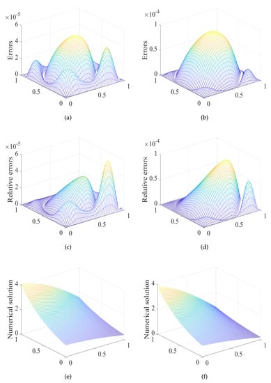
Figure 5. The errors, relative errors and numerical solutions of the AAI algorithm at $z=1/3,2/3$ when $l=m=s=51,h=1/50,n=150,\omega =1.94$. (a) The errors at $z=1/3$; (b) The errors at $z=2/3$; (c) The relative errors at $z=1/3$; (d) The relative errors at $z=2/3$; (e) The numerical solution at $z=1/3$; (f) The numerical solution at $z=2/3$.

(2) Consider the 3D Poisson equation

$$\frac{{\partial }^{2}u}{\partial x^2}+\frac{{\partial }^{2}u}{\partial y^2}+\frac{{\partial }^{2}u}{\partial z^2}=-3sin\left(x\right)sin\left(y\right)sin\left(z\right),(x,y,z)\in {[0,1]}^3,$$

(40)

with the boundary condition,

$$\begin{array}{c}u(0,y,z)=0;\hfill \\ u(1,y,z)=sin\left(1\right)sin\left(y\right)sin\left(z\right);\hfill \\ u(x,0,z)=0;\hfill \\ u(x,1,z)=sin\left(x\right)sin\left(1\right)sin\left(z\right);\hfill \\ u(x,y,0)=0;\hfill \\ u(x,y,1)=sin\left(x\right)sin\left(y\right)sin\left(1\right).\hfill \end{array}$$

(41)

The exact solution of the 3D Poisson problem (40)–(41) is $u(x,y,z)=sin\left(x\right)sin\left(y\right)sin\left(z\right)$.

Table 5 gives the errors ${\parallel E\parallel }_{\infty }$ of AAI algorithm for the problem 2 with the different values of $\omega$ when $l=m=s=31,h=1/30,n=150$, and Figure 6 shows the errors get nearly the minimum $2.2319\times {10}^{-4}$ while $\omega =1.76$. which show the effect of $\omega$ to the AAI algorithm. Table 6, Table 7 and Table 8 give the iteration numbers and times under some error controls, which also show obviously the presented algorithm has smaller iteration numbers than the Jacobi and Gauss-Seidel methods. The computational times are shorter with the grid points increasing.

Table 5. The errors ${\parallel E\parallel }_{\infty }$ of AAI algorithm based on domain decomposition with the different values of $\omega$ when $l=m=s=31,h=1/30,n=150$.

$\mathit{\omega }$	${\Vert \mathit{E}\Vert }_{\mathit{\infty }}$	$\mathit{\omega }$	${\Vert \mathit{E}\Vert }_{\mathit{\infty }}$
1.0	4.2402 $\times {10}^{-2}$	1.6	3.6712 $\times {10}^{-3}$
1.1	3.4981 $\times {10}^{-2}$	1.7	9.4888 $\times {10}^{-4}$
1.2	2.7756 $\times {10}^{-2}$	1.8	3.9125 $\times {10}^{-4}$
1.3	2.0657 $\times {10}^{-2}$	1.9	5.8138 $\times {10}^{-4}$
1.4	1.3986 $\times {10}^{-2}$	2.0	errors
1.5	8.1573 $\times {10}^{-3}$	–	–

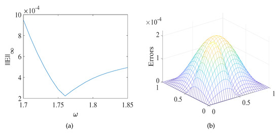
Figure 6. The ${\parallel E\parallel }_{\infty }$ with the different $\omega$ and the errors at $z=0.5$ when $l=m=s=31,h=1/30,n=150$. (a) The errors ${\parallel E\parallel }_{\infty }$ with the different $\omega$; (b) The errors at $z=0.5$ when $\omega =1.76$.

Table 6. The iteration numbers and time(s) of Jacobi, Gauss-Seidel and the AAI algorithm under the different error controls when $l=m=s=31,h=1/30$.

${\parallel \mathit{E}\parallel }_{\mathit{\infty }}$	${10}^{-3}$		${10}^{-4}$
	Numbers	Time(s)	Numbers	Time(s)
Jacobi	557	2.6719	976	3.0781
Gauss-Seidel	288	0.8906	498	1.4688
AAI $(\omega =1.96)$	29	5.6719	135	13.9531

Table 7. The iteration numbers and time(s) of Jacobi, Gauss-Seidel and the AAI algorithm under the different error controls when $l=m=s=51,h=1/50$.

${\parallel \mathit{E}\parallel }_{\mathit{\infty }}$	${10}^{-3}$		${10}^{-4}$
	Numbers	Time(s)	Numbers	Time(s)
Jacobi	1548	15.7031	2712	24.1875
Gauss-Seidel	790	8.3594	1372	15.2500
AAI $(\omega =1.96)$	51	14.5469	181	30.2344

Table 8. The iteration numbers and time(s) of Jacobi, Gauss-Seidel and the AAI algorithm under the different error controls when $l=m=s=71,h=1/70$.

${\parallel \mathit{E}\parallel }_{\mathit{\infty }}$	${10}^{-3}$		${10}^{-4}$
	Numbers	Time(s)	Numbers	Time(s)
Jacobi	3034	98.5468	5317	176.6562
Gauss-Seidel	1538	53.5156	2681	92.9531
AAI $(\omega =1.96)$	91	31.7187	201	54.2968

Figure 7 shows the errors, relative errors and numerical solutions of the AAI iterative algorithm based on domain decomposition for the problem 2 at $z=1/3,2/3$ when $l=m=s=51,h=1/50$, $n=150,\omega =1.96$. All of the numerical experiments examine the effectiveness and accuracy of the presented AAI algorithm.

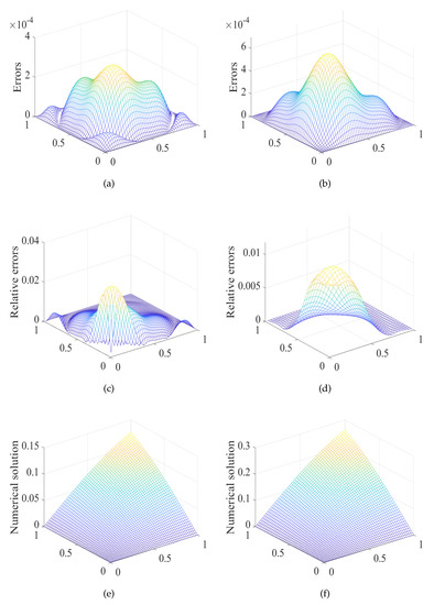
Figure 7. The errors and numerical solutions of the AAI algorithm when $l=m=s=51,h=1/50$, $n=150,\omega =1.96$. (a) The errors at $z=1/3$; (b) The errors at $z=2/3$; (c) The relative errors at $z=1/3$; (d) The relative errors at $z=2/3$; (e) The numerical solution at $z=1/3$; (f) The numerical solution at $z=2/3$.

Since the presented AAI algorithm based on domain decomposition is constructed by the asymmetrical iterative schemes and GE method, which has interior parallelism and is easy to be implemented. During the process of the implementation of the AAI algorithm, there’s no need to solve the large-scale sparse block tridiagonal matrices. When the iteration numbers are odd or even, we just to solve the 3D problems by the constructed iterative schemes, which are computed independently. Once the interfaces are solved by GE method, the other grid points can also be solved by the constructed iterative schemes directly and in parallel. Therefore, the key of parallel implementation lies in information transfer and time cost of the inner boundary. In fact, the whole computation is explicit but convergent, which save the most of the consuming time.

So In this paper, we use the Matlab software to implement the presented AAI algorithm. We extend this idea to solve the other time-dependent high-dimensional problems, and compare the times, speedup, caches and so on. The detailed parallel implementation and performance analysis are provided in [27].

6. Conclusions

In this paper, we provide a new alternating asymmetric iterative (AAI) algorithm for 3D Poisson problem based on domain decomposition. We use several asymmetrical iterative schemes to solve the sub-domains respectively. Meanwhile the asymmetrical iterative schemes are alternatively used on odd and even iteration levels to improve the accuracy. Moreover, we give the convergence of the algorithm and the optimal relaxation factor. Finally, several numerical experiments are taken to examine the effectiveness and accuracy of the presented algorithm.

The study will be extended to other high-dimensional diffusion problems and wave problems and so on, and also can be used to solve on more multi-subdomains, and the corresponding new algorithms will be designed. we will report these soon.

References

- Saad, Y. Iterative Methods for Sparse Linear Systems, 2nd ed.; SIAM: Philadelphia, PA, USA, 2003. [Google Scholar]
- Ge, Y.; Cao, F.; Zhang, J. A transformation-free HOC scheme and multigrid method for solving the 3D Poisson equation on nonuniform grids. J. Comput. Phys. 2013, 234, 199–216. [Google Scholar] [CrossRef]
- Abide, S.; Zeghmati, B. Multigrid defect correction and fourth-order compact scheme for Poisson equation. Comput. Math. Appl. 2017, 73, 1433–1444. [Google Scholar] [CrossRef][Green Version]
- Fen, H.; Zhang, B.L.; Liu, Y. Mathematics Stencil of the finite difference method for Poisson equation and its application. China Sci. 2005, 35, 901–909. (In Chinese) [Google Scholar]
- Spotz, W.F.; Carey, G.F. A high-order compact formulation for the 3D Poisson equation. Numer. Methods Part. Diff. Equ. 1996, 12, 235–243. [Google Scholar] [CrossRef]
- Gupta, M.M.; Kouatchou, J. Symbolic derivation of finite difference approximations for the three dimensional Poisson equation. Numer. Methods Part. Diff. Equ. 1998, 14, 593–606. [Google Scholar] [CrossRef]
- Romao, E.C.; Campos, M.D.; Moura, L.F.M. Application of the galerkin and least-squares finite element methods in the solution of 3D Poisson and Helmholtz equations. Comput. Math. Appl. 2011, 62, 4288–4299. [Google Scholar] [CrossRef][Green Version]
- Nintcheu Fata, S. Semi-analytic treatment of the three-dimensional Poisson equation via a Galerkin BIE method. J. Comput. Appl. Math. 2011, 236, 1216–1225. [Google Scholar] [CrossRef]
- Shi, Z.; Cao, Y.Y.; Chen, Q.J. Solving 2D and 3D Poisson equations and biharmonic equations by the Haar wavelet method. Appl. Math. Model. 2012, 36, 5143–5161. [Google Scholar] [CrossRef]
- Shi, Z.; Cao, Y.Y. A spectral collocation method based on Haar wavelets for Poisson equations and biharmonic equations. Appl. Math. Model. 2011, 54, 2858–2868. [Google Scholar] [CrossRef]
- Speyer, G.; Vasileska, D.; Goodnick, S.M. Efficient Poisson equation solvers for large scale 3D simulations. In Proceedings of the 2001 International Conference on Modeling and Simulation of Microsystems-MSM, Hilton Head Island, SC, USA, 19–21 March 2001; pp. 23–26. [Google Scholar]
- Pedro, V.-L.; Alfredo, P.; Manuel, P.-M. Fast finite difference Poisson solvers on heterogeneous architectures. Comput. Phys. Commun. 2014, 185, 1265–1272. [Google Scholar]
- Pedro, V.-L.; Alfredo, P.; Julien, F.; Manuel, P.-M. Block tridiagonal solvers on heterogeneous architectures. In Proceedings of the 2012 IEEE 10th International Symposium on Parallel and Distributed Processing with Applications, Leganes, Spain, 10–13 July 2012; pp. 609–617. [Google Scholar]
- Stone, C.P.; Duque, E.P.N.; Zhang, Y.; Car, D.; Owens, J.D.; Davis, R.L. 20th AIAA Computational Fluid Dynamics Conference. AIAA-306 2011, 3221, 307. [Google Scholar]
- Yang, W.D.; Li, K.L.; Li, K.Q. A parallel solving method for block-tridiagonal equations on CPUCGPU heterogeneous computing systems. J. Supercomput. 2017, 73, 1760–1781. [Google Scholar] [CrossRef]
- Zhang, Y.; Cohen, J.; Owens, J.D. Proceedings of the 15th ACM SIGPLAN Symposium on Principles and Practice of Parallel Programming; ACM: New York, NY, USA, 2010; p. 127. [Google Scholar]
- Davidson, A.; Zhang, Y.; Owens, J.D. IEEE International Parallel and Distributed Processing Symposium; IEEE: Piscataway, NJ, USA, 2011; p. 956. [Google Scholar]
- Zhang, B.L.; Yuan, G.X.; Liu, X.P. Parallel Finite Difference Methods for Partial Differential Equations; Science Press: Beijing, China, 1994; pp. 7–67. [Google Scholar]
- Mohanty, R.K. The samrt-BLAGE algorithm for singularly perturbed 2D elliptic partial differential equations. Appl. Math. Comput. 2007, 190, 321–331. [Google Scholar]
- Tavakoli, R.; Davami, P. A new parallel Gauss-Seidel method based on alternating group explicit method and domain decomposition method. Appl. Math. Comput. 2007, 188, 713–719. [Google Scholar] [CrossRef]
- Abdullah, A.R.; Ali, N.M. The comparative study of parallel alternating-type iterative methods. Appl. Math. Comput. 1996, 74, 331–344. [Google Scholar]
- Keyes, D.E.; Gropp, W.D. A comparison of domain decomposition on techniques for elliptic partial differential equations and their parallel implementation. SIAM J. Sci. Stat. Comput. 1987, 8, s166–s202. [Google Scholar] [CrossRef]
- Kuznetsov, Y. New algorithm for approximate realization of implicit difference scheme. Soviet J. Numer. Anal. Math. Model. 1988, 3, 99–114. [Google Scholar] [CrossRef]
- Xu, Q.Y.; Wang, W.Q. Wenqiang, W. A new parallel iterative algorithm for solving 2D Poisson equation. Numer. Methods Part. Differ. Eqs. 2011, 27, 829–853. [Google Scholar] [CrossRef]
- Ng, K.F.; Mohd Ali, N.H. Performance analysis of explicit group parallel algorithms for distributed memory multicomputer. Parallel Comput. 2008, 34, 427–440. [Google Scholar] [CrossRef]
- Evans, D. Alternating group explicit method for the diffusion equations. Appl. Math. Model. 1985, 9, 201–206. [Google Scholar] [CrossRef]
- Xu, Q.Y.; Liu, Z.Y. On the parallel implementation of several iterative algorithms for the 3D Poisson and Diffusion problems. 2020; in preparation. [Google Scholar]
© 2020 by the authors. Licensee MDPI, Basel, Switzerland. This article is an open access article distributed under the terms and conditions of the Creative Commons Attribution (CC BY) license (http://creativecommons.org/licenses/by/4.0/).