Abstract
In this paper, we provide tight linear lower bounding functions for multivariate polynomials given over boxes. These functions are obtained by the expansion of polynomials into Bernstein basis and using the linear least squares function. Convergence properties for the absolute difference between the given polynomials and their lower bounds are shown with respect to raising the degree and the width of boxes and subdivision. Subsequently, we provide a new method for constructing an affine lower bounding function for a multivariate continuous rational function based on the Bernstein control points, the convex hull of a non-positive polynomial s, and degree elevation. Numerical comparisons with the well-known Bernstein constant lower bounding function are given. Finally, with these affine functions, the positivity of polynomials and rational functions can be certified by computing the Bernstein coefficients of their linear lower bounds.
1. Introduction
Finding a linear lower bounding function for a nonlinear function is of paramount importance in numerical optimization when a branch and bound approach is used; see [1,2,3]. Bernstein polynomials and their bounding functions were used in a huge variety of problems; see [4,5]. Different methods of minimization and deriving a lower bound have been attacked previously by the expansion of a given polynomial into Bernstein form [1,6,7,8,9,10]; until now, the best lower bound is a linear function relying on the control points and the convex hull property; which is illustrated in Figure 1. Affine lower bounding functions for polynomials on a box were studied in [9], however without any proof of the convergence for the error bound between the affine lower bound and its (monomial) polynomial. In this paper, we aim to improve the linear least squares function derived from Bernstein coefficients and then filling the gap of convergence. Our results lean upon the well-known positivity certificates [11,12,13,14], given by Bernstein’s theorem. Specifically, we raise the number of control points to design a tight affine lower bounding function over a given box. This ensures the positivity of a polynomial in the monomial form and its lower bound at the convergence point.
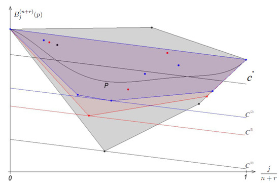
Figure 1.
The curve of a polynomial p of fifth degree, the convex hulls (colored) of its control points (marked by colored points), and examples of affine lower bounding functions for
On the other hand, the Bernstein approach was extended to a rational function in [15,16,17]. Rational functions play an important role in the stability analysis of nonlinear systems, since the system can be stable with a rational control function [18]. Many researchers were focused on the subject of stability analysis for nonlinear systems [19,20]. This topic continues to be a challenging problem. Recently, the stability of nonlinear systems has been translated to positivity certificates [13]. To this end, the coefficients of the Bernstein form of a given rational function R over a specific box of interest tightly bound the range (maximum and minimum value) of R; see [16]. Constant bounds are unreliable, giving extremely poor bounding functions. In this paper, we introduce a new method for constructing a lower bounding function for a multivariate R over boxes. This linear function ensures approximating the given R over the whole domain from below well, which is easier to approximate than the multivariate R and provides positivity certificates linearly. Finally, the tested examples show that the computed error bound of the new method is decreasing as much as we elevate the degree of the Bernstein basis. Summarizing, our contributions are as follows.
- Most of the previous Bernstein lower bound studies focused on bounding functions without providing the rate of convergence [1,7,8,9,10]. In this paper, we provide linear lower bounds for multivariate polynomial functions with a linear and quadratic rate of convergence to the original function over a box.
- Moreover, we certify if the monomial polynomial form is positive and obtain positivity certificates in the Bernstein basis by computing Bernstein coefficients for its linear lower bound.
- Last, we provide the necessary and sufficient conditions for the existence of tight lower bounds for rational polynomial functions given over boxes through Bernstein basis approximations under some maximum degree. Subsequently, the problem of finding upper bounds for the minimum absolute error is not sought after here.
The paper is organized as follows: In the next section, we recall the most important background of Bernstein expansion. In Section 3, we provide a tight linear lower bounding function for polynomials. A tight lower bounding function for rational functions is given in Section 4. Finally, Section 5 gives the conclusions.
2. Bernstein Background
In this section, we introduce the form of polynomials in the Bernstein basis, in the state space, and highlight important properties. First, we consider the Bernstein approach of a polynomial function F expanded over a general l-dimensional box Q in the real intervals set
with:
The width of any is denoted by ,
Let be the maximum width of a box, where
Throughout this paper, the considered Bernstein form is called the tensorial polynomial Bernstein form. We define the arithmetic operations of multiple indices as component-wise. For and a multi-index j, its monomial is . For , we have and . An l-variate polynomial function F is expressed in the monomial form as and can be expressed in the Bernstein basis by:
We underline that zero (sometimes one) is the multi-index with all components equal to zero (equal to one).
Moreover, the Bernstein coefficients of F of degree n over Q are given by the formula:
where:
Remark 1.
The Bernstein basis polynomials are non-negative for all , i.e., , .
Without loss of generality, we can consider the domain of F to be the unit box , since any non-empty box in can be transformed thereupon by a linear transformation. Hence, the expression of F as (1) can be simplified with:
and:
Let us highlight three important properties of Bernstein polynomials:
(i) The endpoint interpolation property:
for some , satisfies , .
(ii) The convex hull, which states that the graph of F over U is contained within the convex hull of the control points derived from the Bernstein coefficients, i.e.,
where conv denotes the convex hull.
(iii) The enclosing property:
for all .
Remark 2.
([21], degree elevation) The Bernstein basis of degree n can be expressed in terms of those of degree , where , , as:
It follows by [22] that:
Remark 3.
Let a multivariate polynomial F be of degree with components , . If the Bernstein degree is elevated so that are the Bernstein coefficients of degree , . Then, we have:
3. Lower Bounds for Polynomials
The Bernstein linear least squares function was addressed in [9]. This yields an affine function that closely approximates polynomials on the whole box.
Let D be the matrix of rows and columns where the element is defined as:
Let A be the vector consisting of the corresponding Bernstein coefficients. Then, the coefficients of the linear least squares approximation of all the control points are given by the solution to:
yielding the affine function:
For numerically reliable approaches to solve the linear least squares problem, we refer the readers to consult [23]. A valid linear lower bounding function is obtained by performing a downward shift:
where:
3.1. Tight Bounding Functions
Providing positivity certificates in the tensorial Bernstein basis for designing control systems for polynomial dynamic systems requires bounding the given polynomial from below. These bounds can be given in the BP where computing the coefficients is only linear. In this section, we improve the lower bounding function (9) by applying Remark 3 on the linear least squares function and then decreasing the downward shift. By Remark 2, if the degree of the Bernstein expansion of is elevated, then Bernstein coefficients of order , can easily be computed as convex combinations of the coefficients of order n. It follows that for any vector with components , ,
When we assume that is a non-zero, then by using Remark 3, a tight bounding function is obtained by performing a downward shift:
This method approximates the original function well, preserves the broad shape of F on the whole box, and obtains the convergence properties; see Figure 1.
3.2. Tight Error Values
To guarantee that the bounding function approximates the polynomial from below well, we show that the minimum error bound (between (11) and ) is decreasing with respect to raising the degree.
Remark 4.
By (10) and since the Bernstein coefficients are monotone (Remark 2), the lower bounding function is increasing with respect to raising r.
Theorem 1.
For any polynomial function F with its lower bound , the following error bound holds:
Proof.
By using Theorem 1 and applying Remark 4 to the minimum error bound, the following corollary holds.
Corollary 1.
The minimum error bound is decreasing with respect to raising r. In fact,
3.3. Linear Convergence
In this subsection, we show that the absolute difference between the lower bound and the original polynomial is linearly convergent if the degree of Bernstein basis is elevated. We start with the following theorem, which extends [2], Theorem 3, to the multivariate case.
Theorem 2.
([6], Theorem 4.3.1) For with , , the following bound holds for the overestimation of the range of F over U by the Bernstein form:
where:
is independent of the elevated maximum Bernstein degree .
Theorem 3.
Given that is the tight lower bound of F over U, then:
where M is the maximum elevated degree of the Bernstein basis of F and .
3.4. Quadratic Convergence on a Box
In this subsection, the quadratic convergence of the minimum absolute difference between and F with respect to the width of Q is shown.
Remark 5.
Where , the bound on the right-hand side of (14) can be improved slightly; see [10], Formula (17). Let in Q be a grid point with the component in , ,
Then, the difference can be bounded from above for all by , where is a constant that can be given explicitly by (15); see [24], Corollary 3.4.16. This illustrates that the discrete polynomial function converges linearly and quadratically to the corresponding Bernstein coefficients. This result will be used in the proof of the following theorem.
Theorem 4.
Let Y be fixed from the unit real interval space of l dimensions, . Then, for all , , it holds that:
where is independent of Q.
Proof.
Assume that:
is attained at for some , with the corresponding grid point . Then:
where the first inequality follows since is a grid point in Q, and the last one is reached by using Remark 5. □
3.5. Quadratic Convergence by Subdivision
The convergence of the error bound between and F is only linear if we raise the degree. Instead, if we subdivide U, we obtain quadratic convergence with respect to subdivision. Repeated bisection of in all coordinate directions results at the subdivision level in sub-boxes of edge length , ; see [15,25]. The following theorem provides the quadratic convergence with respect to subdivision U.
Theorem 5.
Let be the tight lower bounding function of F over . Then, for each ,
where is an independent constant of d, which can be given explicitly by (15).
Proof.
The proof of this theorem can be obtained by using similar arguments used in the proof of Theorem 4. □
3.6. Multi-Affine Function
The linear least squares function in (9) and (11) is constructed from the Bernstein control points of a fixed degree n, , whereas just the convergence properties of the tight bound (11) is obtained by elevating the degree. In this subsection, we improve the linear least squares function to be computed from the control points of degree and then compute the maximum positive discrepancy between and the control points:
The tight bounding function can be improved by performing a downward shift:
The linear least squares function in this bound is very accurate since the number of control points can be raised as long as we elevate the degree r. Finally, the convergence properties for the absolute error of this developed affine bound (20) and F can be similarly proven by using arguments similar to those given in the proof of Theorems 3–5.
4. Bounding Functions for Rational Functions
Let be a rational function where p and g are multivariate polynomials of degree , with Bernstein coefficients of the same degree.
For and the multi-index zero, we use the notation:
Without loss of generality, we may assume that the Bernstein coefficients are positive. The easiest type of affine lower bounding function is one equal to a constant; we can simply assign it the value of the minimum rational Bernstein coefficient:
Then, according to the range enclosing [16] of a rational function:
Remark 6.
Given that is the constant lower bounding function (22) of , then the following error bound is valid:
However, constant bounding functions do not approximate the broad shape of the rational function over the whole box; see Figure 2.
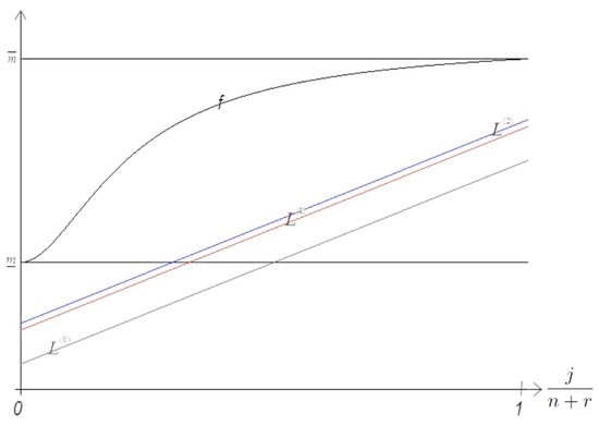
Figure 2.
The curve of a rational function f of second degree and an example tight lower bounding function for
4.1. Affine Bounds for Rational Functions
The Bernstein expansion of a given non-positive polynomial s introduces a method for constructing linear lower bounding functions for rational functions based on the control points; using a linear least squares approximation of the entire control point structure and degree elevation. Such bounds are tight and broadly shape preserving.
The rational Bernstein form of R of degree is given as:
Without loss of generality, we assume throughout the paper that , .
We recall from Proposition 4 in [15] that:
Hence, . Therefore, we can define the following non-positive polynomial:
Therefore, the Bernstein coefficients of s of degree are given by:
Since the Bernstein enclosure bound of is monotone and by applying (11) to , a tight lower bounding function of a rational function R is obtained by:
where:
and:
This method is easier to approximate than the nonlinear rational function and approximates over the whole domain; see Figure 2.
4.2. Rational Error Bound
In this subsection, we show that is increasing with respect to raising the degree of the Bernstein form.
Remark 7.
Given that is the tight lower bound of R; then the following error bound is valid,
Lemma 1.
The lower bounding function is increasing with respect to raising r.
Proof.
By applying Lemma 1 to the minimum difference between R and , the following corollary holds.
Corollary 2.
The rational minimum error bound is decreasing with respect to raising r. Precisely,
4.3. Numerical Results
The simple constant bounding function of rational functions is tight at the convergence point. However, a constant bound is crude, and we expect it to exhibit a mediocre error bound. In general, it does not optimize the rational functions over the whole box as closely as the tight linear lower bound (25).
Example 1.
We consider the following two rational functions, , from [7] and [16].
and:
where:
We list in Table 1 the minimum error bound of the rational constant bounding method (22), and , , of the new method (25). The new method is superior to the constant method for where . The constant method is superior to the new method for where . Despite this, it can be seen that the absolute distance between and is decreasing as long as we elevate the degree. Furthermore, Figure 2 illustrates the linear optimization over the hole domain.

We implemented our numerical results and figures using , OpenCV, and QT libraries. Bernstein coefficients were computed by software of the general Bernstein coefficients.
5. Conclusions
In this paper, we improved a linear lower bounding function for a polynomial over boxes. This function was mainly obtained by using the linear least squares function of the Bernstein control points. We proved the linear and quadratic rates of convergence between the original functions and their improved lower bounding functions. Therefore, computing positivity certificates for the stability of polynomial systems was improved. This was since computing polynomial positive values in our method became linear in the Bernstein form. On the other hand, we constructed affine lower bounding functions for rational functions, which could be applied in global optimization problems and the stability of dynamic systems with rational control. The approach is suited to many rational functions that appear in typical global optimization problems; even if the number of parameters in the problem was big, the number that appears in any given constraint function was much less. Finally, we provided sufficient conditions for the rational convergence properties and decreasing of the new method error bounds.
Author Contributions
Formal analysis, investigation, and writing-original draft preparation, T.H., M.A. and H.A.-Z. All authors have read and agreed to the published version of the manuscript.
Funding
This research received no external funding.
Acknowledgments
The authors gratefully acknowledge support from Al-Zaytoonah University of Jordan under Grant Number 2019-2018/585/G12. The first author would like to thank Monssef Alsweis (University of Konstanz) for his implementations and careful reading of the manuscript.
Conflicts of Interest
The authors declare no conflict of interest.
References
- Cargo, G.; Shisha, O. The Bernstein form of a polynomial. J. Res. 1966, 70, 79–81. [Google Scholar] [CrossRef]
- Garloff, J. Convergent bounds for the range of multivariate polynomials. In Interval Mathematics 1985; Nickel, K., Ed.; Springer: Berlin/Heidelberg, Germany, 1986; pp. 37–56. [Google Scholar]
- Hansen, E.; Walster, G.W. Global Optimization Using Interval Analysis: Revised and Expanded; CRC Press: Boca Raton, FL, USA, 2003; Volume 4, pp. 379–456. [Google Scholar]
- Hamadneh, T. Bounding Polynomials and Rational Functions in the Tensorial and Simplicial Bernstein Forms. Ph.D. Thesis, University of Konstanz, Konstanz, Germany, 2018. [Google Scholar]
- Farouki, R.T. The Bernstein polynomial basis: A centennial retrospective. Comput. Aided Geom. Des. 2012, 29, 379–419. [Google Scholar] [CrossRef]
- Hamadneh, T.; Athanasopoulos, N.; Ali, M. Minimization and Positivity of the Tensorial Rational Bernstein Form. In Proceedings of the 2019 IEEE Jordan International Joint Conference on Electrical Engineering and Information Technology (JEEIT), Amman, Jordan, 9–11 April 2019; pp. 474–479. [Google Scholar]
- Garloff, J.; Schabert, A.; Smith, A.P. Bounds on the range of multivariate rational functions. PAMM 2012, 12, 649–650. [Google Scholar] [CrossRef]
- Garloff, J.; Smith, A.P. A comparison of methods for the computation of affine lower bound functions for polynomials. In Global Optimization and Constraint Satisfaction; Springer: Berlin/Heidelberg, Germany, 2003; pp. 71–85. [Google Scholar]
- Garloff, J.; Smith, A.P. Rigorous affine lower bound functions for multivariate polynomials and their use in global optimisation. Konstanzer Schriften in Mathematik und Informatik 2008, 250, 1–14. [Google Scholar]
- Rivlin, T.J. Bounds on a polynomial. J. Res. Nat. Bur. Stand. Sect. B. 1970, 74, 47–54. [Google Scholar] [CrossRef]
- Bochnak, J.; Coste, M.; Roy, M.F. Real Algebraic Geometry; Springer: Berlin/Heidelberg, Germany, 1998. [Google Scholar]
- Powers, V. Positive polynomials and sums of squares: Theory and practice. Real Algebraic Geometry 2011, 1, 78–149. [Google Scholar]
- Hamadneh, T.; Wisniewski, R. The Barycentric Bernstein Form for Control Design. In Proceedings of the 2018 Annual American Control Conference (ACC), Washington, DC, USA, 17–19 June 2018; pp. 3738–3743. [Google Scholar]
- Hamadneh, T.; Wisniewski, R. Algorithm for Bernstein Polynomial Control Design. In Proceedings of the 6th IFAC Conference on Analysis and Design of Hybrid Systems ADHS 2018, Oxford, UK, 11–13 July 2018; Volume 51, pp. 283–289. [Google Scholar]
- Garloff, J.; Hamadneh, T. Convergence and Inclusion Isotonicity of the Tensorial Rational Bernstein Form. In Scientific Computing, Computer Arithmetic, and Validated Numerics; Springer: Berlin, Germany, 2015; pp. 171–179. [Google Scholar]
- Narkawicz, A.; Garloff, J.; Smith, A.P.; Munoz, C.A. Bounding the Range of a Rational Functiom over a Box. Reliab. Comput. 2012, 17, 34–39. [Google Scholar]
- Titi, J.; Hamadneh, T.; Garloff, J. Convergence of the Simplicial Rational Bernstein Form. In Modelling, Computation and Optimization in Information Systems and Management Sciences; Springer: Berlin, Germany, 2015; pp. 433–441. [Google Scholar]
- Vatani, M.; Hovd, M. Lyapunov stability analysis and controller design for rational polynomial systems using sum of squares programming. In Proceedings of the 2017 IEEE 56th Annual Conference on Decision and Control (CDC), Melbourne, Australia, 12–15 December 2017; pp. 4266–4271. [Google Scholar]
- Ackerman, J. Robust Control; Springer: London, UK, 1993. [Google Scholar]
- Nersesov, S.G.; Haddad, W.M. On the stability and control of nonlinear dynamical systems via vector Lyapunov functions. IEEE Trans. Autom. Control 2006, 51, 203–215. [Google Scholar] [CrossRef]
- Farouki, R.T.; Rajan, V. On the numerical condition of polynomials in Bernstein form. Comput. Aided Geom. Des. 1987, 4, 191–216. [Google Scholar] [CrossRef]
- Farin, G.E. Triangular Bernstein-Bézier patches. Comput. Aided Geom. Des. 1986, 3, 83–127. [Google Scholar] [CrossRef]
- Björck, Å. The calculation of linear least squares problems. Acta Numer. 2004, 13, 1–53. [Google Scholar] [CrossRef]
- Stahl, V. Interval Methods for Bounding the Range of Polynomials and Solving Systems of Nonlinear Equations. Ph.D. Thesis, Johannes Kepler Universität, Linz, Austria, 1995. [Google Scholar]
- Zettler, M.; Garloff, J. Robustness analysis of polynomials with polynomial parameter dependency using Bernstein expansion. IEEE Trans. Autom. Control. 1998, 43, 425–431. [Google Scholar] [CrossRef]
© 2020 by the authors. Licensee MDPI, Basel, Switzerland. This article is an open access article distributed under the terms and conditions of the Creative Commons Attribution (CC BY) license (http://creativecommons.org/licenses/by/4.0/).