Bivariate Burr X Generator of Distributions: Properties and Estimation Methods with Applications to Complete and Type-II Censored Samples

Abstract

Burr proposed twelve different forms of cumulative distribution functions for modeling data. Among those twelve distribution functions is the Burr X distribution. In statistical literature, a flexible family called the Burr X-G (BX-G) family is introduced. In this paper, we propose a bivariate extension of the BX-G family, in the so-called bivariate Burr X-G (BBX-G) family of distributions based on the Marshall–Olkin shock model. Important statistical properties of the BBX-G family are obtained, and a special sub-model of this bivariate family is presented. The maximum likelihood and Bayesian methods are used for estimating the bivariate family parameters based on complete and Type II censored data. A simulation study was carried out to assess the performance of the family parameters. Finally, two real data sets are analyzed to illustrate the importance and the flexibility of the proposed bivariate distribution, and it is found that the proposed model provides better fit than the competitive bivariate distributions.

1. Introduction

The Burr X (BX) model, as one of twelve models, was explored by utilizing the method of differential equation (see [1]). The random variable X is said to have the BX if its cumulative distribution function (CDF) is given by

$$F_{BX}(x;\gamma )={\left[1-e^{-x^2}\right]}^{\gamma };x>0,$$

(1)

where $\gamma >0$ is the shape parameter. This model has found many applications in many areas such as reliability study, agricultural, biological, health, the lifetime of random phenomenon and engineering, see for example, [2,3,4,5,6,7,8].

Reference [9] introduced the Burr X-G (BX-G) family based on [10] technique, where [10] proposed a general form to generate a new family named the transformed-transformer (T-X) family. Thus, the random variable X is said to have the BX-G family if its CDF is given by

$$F_{BX-G}(x;\mathit{\omega },\gamma )={\left[1-e^{-{\left(\frac{G(x;\mathit{\omega })}{\overline{G}(x;\mathit{\omega })}\right)}^2}\right]}^{\gamma };x>0,$$

(2)

where $G(x;\mathit{\omega })$ is the baseline CDF, $\overline{G}(x;\mathit{\omega })=1-G(x;\mathit{\omega })$, and $\mathit{\omega }$ is a vector of parameters (1$\times k$). The corresponding probability density function (PDF) to Equation (2) can be expressed as

$$f_{BX-G}(x;\mathit{\omega },\gamma )=\frac{2\gamma g(x;\mathit{\omega })G(x;\mathit{\omega })}{{\left(\overline{G}(x;\mathit{\omega })\right)}^3}{e}^{-{\left(\frac{G(x;\mathit{\omega })}{\overline{G}(x;\mathit{\omega })}\right)}^2}{\left[1-e^{-{\left(\frac{G(x;\mathit{\omega })}{\overline{G}(x;\mathit{\omega })}\right)}^2}\right]}^{\gamma -1};x>0,$$

(3)

where $g(x;\mathit{\omega })$ is the baseline PDF.

Many authors used [10] technique to build new models for the following reasons: to make the kurtosis more flexible compared to the baseline model, to construct heavy-tailed distributions for modeling real data, to generate distributions with symmetric, left-skewed, right-skewed or reversed-J shape, to define special models with all types of the hazard rate function and to provide consistently better fits than other generated models under the same baseline distribution, see for example, odd Burr generalized-G family by [11], a new Weibull-G family by [12], generalized odd log-logistic-G family by [13], odd Lindley-G family by [14], odd flexible Weibull-H family by [15], odd log-logistic Lindley-G family by [16], odd Chen generator by [17] and references cited therein.

The bivariate distributions have been derived, developed and discussed by many authors which have wide applications in the fields of reliability (lifetime and stress–strength of components), sports, engineering, weather and drought, more detail is given in [18,19]. The construction or development of bivariate distributions are mainly via: the marginals, copulas, compounding, reduction and conditioning. The trend in proposing new bivariate compounded (power series family) and generalized (G-) families of distributions has received increased attention, which is briefly described below:

• Bivariate compounded distributions and families: Reference [20] obtained four bivariate extended exponential-geometric distributions from the extended exponential-geometric model introduced by [21]. Reference [22] compounded two discrete distributions and proposed bivariate geometric-Poisson distribution. Reference [23] proposed the bivariate Weibull-geometric distribution and discussed some of its properties and estimation methods. Reference [24] proposed the bivariate exponentiated generalized Weibull–Gompertz distribution. Reference [25] proposed the bivariate exponentiated modified Weibull extension distribution. Reference [26] introduced and studied complementary bivariate generalized linear failure rate-power series family of distributions.
• Bivariate G-families: Reference [27] introduced bivariate proportional reversed hazard rate family. Reference [28] proposed three bivariate beta-generated families. Reference [29] introduced bivariate Zografos–Balaktishnan gamma-G family. Reference [30] proposed Marshall–Olkin type bivariate exponentiated extended Weibull family. Reference [31] proposed bivariate Ristić–Balaktishnan gamma-G family. Reference [32,33,34] introduced three bivariate families (bivariate Gumbel-G family, bivariate Weibull-G family and bivariate Gompertz-G family).

The aim of our paper was to introduce a new bivariate family, the bivariate Burr X-G (BBX-G) family based on the Marshall–Olkin shock model (see [35]), whose marginal distributions are BX-G families. The structure of the proposed paper follows similarly to that of [32,33]. A random vector $\mathit{X}=(X_1,X_2)$ follows the bivariate Marshall–Olkin model if and only if there exist three independent random variables $U_1$, $U_2$ and $U_3$ such that ($X_1=max(U_1,U_3)$ and $X_2=max(U_2,U_3)$) or ($X_1=min(U_1,U_3)$ and $X_2=min(U_2,U_3)$). The proposed BBX-G family is constructed from three independent BX-G families using a maximization process. Our reasons for introducing the BBX-G family are the following:

• The joint CDF can be expressed as a mixture of an absolute continuous distribution function and a singular distribution function.
• The joint PDF, joint CDF and joint reliability function (RF) are in closed forms, which make it proper to use in practice.
• The joint PDF and joint hazard rate function can take different shapes depending on the parameter values.
• The marginals can be used to analyze different types of hazard rates.
• The stress–strength model does not depend on the baseline function, but only on the model parameters.
• This class can be used as a stress model or as a maintenance model.
• This class contains several special bivariate models depending on the baseline G.
• This class can be used to model skewed data sets.

The paper is structured as follows. In Section 2, the BBX-G family and its marginals are defined. Some mathematical properties of the BBX-G family of distributions such as Marshall–Olkin copula, median correlation coefficient, moments, product moment, covariance, skewness, kurtosis, joint reliability function, joint hazard and reversed hazard rates and stress–strength reliability are obtained in Section 3. In Section 4, a special sub-model of this bivariate family is presented in detail. The family parameters are estimated by maximum likelihood and Bayesian methods based on complete and Type-II censored samples. Moreover, bootstrap confidence intervals are reported in Section 5. In Section 6, a simulation study is presented. The usefulness of the new bivariate family of distributions is illustrated by means of a real data set, where we prove empirically that our proposed model outperforms some well-known bivariate distributions in Section 7. Section 8 offers some concluding remarks. Finally, abbreviation and preliminary Sections are listed in Appendix A.

2. The BBX-G Family and Its Marginal Functions

Assume $U_i\sim BX-G$$(\mathit{\omega },{\gamma }_i);i=1,2,3$are three independent random variables. Define $X_d=max\{U_d,U_3\}$$;d=1,2$. Then, the joint CDF of the BBX-G family can be proposed as

$$F_{X_1,X_2}(x_1,x_2)=F_{BX-G}(z;\mathit{\omega },{\gamma }_3){\displaystyle \prod _{i=1}^2}{F}_{BX-G}(x_i;\mathit{\omega },{\gamma }_i),$$

(4)

where$z=min(x_1,x_2).$ The corresponding joint PDF can be expressed as follows

$$f_{X_1,X_2}(x_1,x_2)=\left\{\begin{array}{c}{f}_1(x_1,x_2)\mathrm{if}0<x_1<x_2<\infty \hfill \\ f_2(x_1,x_2)\mathrm{if}0<x_2<x_1<\infty \hfill \\ f_0\left(x\right)\mathrm{if}0<x_1=x_2=x<\infty ,\hfill \end{array}\right.$$

(5)

where

$$f_1(x_1,x_2)=f_{BX-G}\left(x_2;\mathit{\omega },{\gamma }_2\right)\times f_{BX-G}\left(x_1;\mathit{\omega },{\gamma }_1+{\gamma }_3\right),$$

$$f_2(x_1,x_2)=f_{BX-G}\left(x_1;\mathit{\omega },{\gamma }_1\right)\times f_{BX-G}\left(x_2;\mathit{\omega },{\gamma }_2+{\gamma }_3\right)$$

and

$$f_0\left(x\right)=\frac{{\gamma }_3}{{\gamma }_1+{\gamma }_2+{\gamma }_3}{f}_{BX-G}\left(x;\mathit{\omega },{\gamma }_1+{\gamma }_2+{\gamma }_3\right).$$

The expressions $f_i(x_1,x_2)$, $i=1,2$ can be obtained by differentiating Equation (4) with respect to $x_i$, $i=1,2$. But we can use the following fact to get $f_0\left(x\right)$

$${\displaystyle \underset{0}{\overset{\infty }{\int }}}{f}_0\left(x\right)dx+{\int }_0^{\infty }{\int }_0^{x_2}{f}_1(x_1,x_2)d{x}_{1}d{x}_2+{\int }_0^{\infty }{\int }_0^{x_1}{f}_2(x_1,x_2)d{x}_{2}d{x}_1=1.$$

(6)

Further, the marginal CDFs for the proposed family can be represented as follows

$$F_{X_i}\left(x_i\right)=F_{BX-G}\left(x_i;\mathit{\omega },{\gamma }_i+{\gamma }_3\right);i=1,2.$$

(7)

The corresponding marginal PDFs can be expressed as follows

$$f_{X_i}\left(x_i\right)=f_{BX-G}\left(x_i;\mathit{\omega },{\gamma }_i+{\gamma }_3\right).$$

(8)

Thus, the conditional probability density function of $X_i$ given $X_j=x_j,$$(i,j=1,2,i\ne j)$ can be expressed as follows

$$f_{X_i\mid X_j}(x_i\mid x_j)=\left\{\begin{array}{c}{f}_{X_i\mid X_j}^{\left(1\right)}(x_i\mid x_j)\mathrm{if}0<x_i<x_j<\infty \hfill \\ f_{X_i\mid X_j}^{\left(2\right)}(x_i\mid x_j)\mathrm{if}0<x_j<x_i<\infty \hfill \\ f_{X_i\mid X_j}^{\left(3\right)}(x_i\mid x_j)\mathrm{if}0<x_i=x_j<\infty ,\hfill \end{array}\right.$$

(9)

where

$$\begin{array}{c}\hfill f_{X_i\mid X_j}^{\left(1\right)}(x_i\mid x_j)=\frac{2{\gamma }_j\left({\gamma }_i+{\gamma }_3\right)g(x_i;\mathit{\omega })G(x_i;\mathit{\omega })e^{-{\left(\frac{G(x_i;\mathit{\omega })}{\overline{G}(x_i;\mathit{\omega })}\right)}^2}{\left(1-e^{-{\left(\frac{G(x_i;\mathit{\omega })}{\overline{G}(x_i;\mathit{\omega })}\right)}^2}\right)}^{{\gamma }_i+{\gamma }_3-1}}{\left({\gamma }_j+{\gamma }_3\right){\left(\overline{G}(x_i;\mathit{\omega })\right)}^3{\left(1-e^{-{\left(\frac{G(x_j;\mathit{\omega })}{\overline{G}(x_j;\mathit{\omega })}\right)}^2}\right)}^{{\gamma }_3}},\\ \hfill f_{X_i\mid X_j}^{\left(2\right)}(x_i\mid x_j)=\frac{2{\gamma }_i}{{\left(\overline{G}(x_i;\mathit{\omega })\right)}^3}g(x_i;\mathit{\omega })G(x_i;\mathit{\omega })e^{-{\left(\frac{G(x_i;\mathit{\omega })}{\overline{G}(x_i;\mathit{\omega })}\right)}^2}{\left(1-e^{-{\left(\frac{G(x_i;\mathit{\omega })}{\overline{G}(x_i;\mathit{\omega })}\right)}^2}\right)}^{{\gamma }_i-1}\end{array}$$

and

$$f_{X_i\mid X_j}^{\left(3\right)}(x_i\mid x_j)=\frac{{\gamma }_3}{{\gamma }_j+{\gamma }_3}{\left(1-e^{-{\left(\frac{G(x_i;\mathit{\omega })}{\overline{G}(x_i;\mathit{\omega })}\right)}^2}\right)}^{{\gamma }_i}.$$

Equation (9) can be obtained by substituting from Equations (5) and (8) in the relation $f_{X_i\mid X_j}(x_i\mid x_j)=\frac{f_{X_i,X_j}(x_i,x_j)}{f_{X_j}\left(x_j\right)},$$(i\ne j=1,2).$ The PDF and CDF marginals can be represented as a linear representation as follows

$$f_{X_i}\left(x_i\right)={\displaystyle \sum _{m,l=0}^{\infty }}{V}_{m,l}^{\left(i\right)}{\mathsf{{\rm Y}}}_{2(m+1)+l}^{\left(i\right)}(x_i;\mathit{\omega });i=1,2$$

(10)

and

$$F_{X_i}\left(x_i\right)={\displaystyle \sum _{m,l=0}^{\infty }}{V}_{m,l}^{\left(i\right)}{\mathsf{\Lambda }}_{2(m+1)+l}^{\left(i\right)}(x_i;\mathit{\omega });i=1,2,$$

(11)

respectively, where ${\mathsf{{\rm Y}}}_{2(m+1)+l}^{\left(i\right)}(x_i;\mathit{\omega })=(2(m+1)+l)g(x_i;\mathit{\omega })G{(x_i;\mathit{\omega })}^{2m+l+1},$

$$V_{m,l}^{\left(i\right)}=\frac{2({\gamma }_i+{\gamma }_3){(-1)}^m\mathsf{\Gamma }({\gamma }_i+{\gamma }_3)\mathsf{\Gamma }(2m+l+3)}{m!l!\left(2\right(m+1)+l)\mathsf{\Gamma }(2m+3)}{\displaystyle \sum _{k=0}^{\infty }}\frac{{(-1)}^k{(k+1)}^m}{k!\mathsf{\Gamma }({\gamma }_i+{\gamma }_3-k)}$$

and ${\mathsf{\Lambda }}_{2(m+1)+l}^{\left(i\right)}$ is the CDF of the exponential-G (exp-G) family with power parameter $2(m+1)+l$. For more detail around exp-G family of distributions (see [36]).

If the bivariate vector $\mathit{X}$∼ BBX-G$(\mathit{\omega },{\gamma }_1,{\gamma }_2,{\gamma }_3)$, then the distribution for each $T=max\{X_1,X_2\}$ and $S=min\{X_1,X_2\}$ can be written as follows

$$F_T\left(t\right)=F_{BX-G}(t;\mathit{\omega },{\gamma }_1+{\gamma }_2+{\gamma }_3)$$

(12)

and

$$F_S\left(t\right)=F_{BX-G}(t;\mathit{\omega },{\gamma }_1+{\gamma }_3)+F_{BX-G}(t;\mathit{\omega },{\gamma }_2+{\gamma }_3)-F_T\left(t\right),$$

(13)

respectively.

3. Statistical Properties

3.1. Marshall–Olkin Copula

It is found that the BBX-G family has both an absolute continuous part on $0<$$x_1\ne x_2$<∞ with weight $\frac{{\gamma }_1+{\gamma }_2}{{\gamma }_1+{\gamma }_2+{\gamma }_3}$ and a singular part along the line $x_1=x_2$ with weight $\frac{{\gamma }_3}{{\gamma }_1+{\gamma }_2+{\gamma }_3}$, similar to Marshall and Olkin’s bivariate exponential model. Moreover, the BBX-G family can be obtained by using the Marshall–Olkin copula with the marginals as the BX-G families. To every $F_{X_1,X_2}(x_1,x_2)$ with continuous marginals $F_{X_1}\left(x_1\right)$ and $F_{X_2}\left(x_2\right)$ corresponds to a unique bivariate distribution function with uniform margins $B:{[0,1]}^2\to [0,1]$ called a copula, such that

$$F_{X_1,X_2}(x_1,x_2)=B\left(F_{X_1}\left(x_1\right),F_{X_2}\left(x_2\right)\right);\mathrm{for}\mathrm{all}(x_1,x_2)\in R^2,$$

(14)

(see [37]). The Marshall–Olkin copula can be written as follows

$$B_{{\delta }_1,{\delta }_2}(D_1,D_2)=D_1^{1-{\delta }_1}{D}_2^{1-{\delta }_2}min\left(D_1^{{\delta }_1},D_2^{{\delta }_2}\right);\mathrm{for}0<{\delta }_1,{\delta }_2<1.$$

(15)

Using $D_i=F_{X_i}\left(x_i\right)$, $X_i\sim BX-G$$(\mathit{\omega },{\gamma }_i+{\gamma }_3)$ and ${\delta }_i=\frac{{\gamma }_3}{{\gamma }_i+{\gamma }_3};i=1,2$ then $B_{{\delta }_1,{\delta }_2}(D_1,D_2)$gives the same CDF as Equation (4) where $B_{{\delta }_1,{\delta }_2}(D_1,D_2)\ge D_1{D}_2$ for all $D_1,D_2$$\in {[0,1]}^2$. Therefore, if ($X_1,X_2$) follow the BBX-G family, then they are positive quadrant dependent (see [38]). For $f_{X_1}(.)$ and $f_{X_2}(.)$, we get $\mathit{Cov}\left\{f_{X_1}\left(X_1\right),f_{X_2}\left(X_2\right)\right\}\ge 0$ (see [39]), where $f_{X_1}(.)$ and $f_{X_2}(.)$ are increasing functions.

3.2. Median Correlation Coefficient

Reference [40] proposed the median correlation coefficient $N_{X_1,X_2}$as a form $N_{X_1,X_2}=4F_{X_1,X_2}(N_{X_1},N_{X_2})-1,$ where $N_{X_1}$ and $N_{X_2}$ denote the median of $X_1$ and $X_2$ respectively. If $X_1\sim BX-G$$(\mathit{\omega },{\gamma }_1+{\gamma }_3)$ and $X_2\sim BX-G$$(\mathit{\omega },{\gamma }_2+{\gamma }_3)$,then

$$N_{X_1,X_2}=\left\{\begin{array}{c}4F_{BX-G}\left(N_{X_2};\mathit{\omega },{\gamma }_2\right)\times F_{BX-G}\left(N_{X_1};\mathit{\omega },{\gamma }_1+{\gamma }_3\right)-1\mathrm{if}{x}_1\le x_2\hfill \\ 4F_{BX-G}\left(N_{X_1};\mathit{\omega },{\gamma }_1\right)\times F_{BX-G}\left(N_{X_2};\mathit{\omega },{\gamma }_2+{\gamma }_3\right)-1\mathrm{if}{x}_1>x_2,\hfill \end{array}\right.$$

(16)

where

$$N_{X_i}=Q_G\left(\frac{1}{\left({\left[-log\left(1-A^{\frac{1}{{\gamma }_i+{\gamma }_3}}\right)\right]}^{-0.5}+1\right)}\right);i=1,2,$$

(17)

and $Q_G(.)=G^{-1}(.)$ is the baseline quantile function for A has a uniform $A(0,1)$ distribution.

3.3. The Moments, Product Moment, Covariance, Skewness and Kurtosis

The rth moment of $X_i$, say $M_i^{\left(r\right)}$, can be defined as $M_i^{\left(r\right)}=\mathit{E}\left(X_i^r\right)={\int }_0^{\infty }{x}_i^r{f}_{X_i}\left(x_i\right)d{x}_i.$ Hence, by using Equation (10), we get

$$\begin{array}{cc}\hfill M_i^{\left(r\right)}& ={\displaystyle \sum _{m,l=0}^{\infty }}{V}_{m,l}^{\left(i\right)}{\displaystyle \underset{0}{\overset{\infty }{\int }}}{x}_i^r{\mathsf{{\rm Y}}}_{2(m+1)+l}^{\left(i\right)}(x_i;\mathit{\omega })d{x}_i\hfill \\ \hfill & ={\displaystyle \sum _{m,l=0}^{\infty }}{V}_{m,l}^{\left(i\right)}\mathit{E}\left(Z_{i,2(m+1)+l}^r\right),\hfill \end{array}$$

(18)

where $Z_{i,2(m+1)+l};i=1,2$ be a random variable having the exp-G CDF with power parameter $2(m+1)+l$. The moments of the exp-G distributions are given by [41]. Setting $r=1$ in Equation (18), we get the mean of $X_i;i=1,2$. Thus, the nth central moment of $X_i$, say $L_i^{\left(n\right)}$, is given by

$$L_i^{\left(n\right)}={\displaystyle \sum _{r=0}^n}{\displaystyle \sum _{m,l=0}^{\infty }}{\left[-M_i^{\left(1\right)})\right]}^{n-r}\left(\begin{array}{c}n\\ r\end{array}\right)V_{m,l}^{\left(i\right)}\mathit{E}\left(Z_{i,2(m+1)+l}^r\right);i=1,2.$$

(19)

The sth incomplete moment of $X_i$, say ${\phi }_i^{\left(s\right)}\left(t_i\right)$, can be defined as ${\phi }_i^{\left(s\right)}\left(t_i\right)={\int }_0^{t_i}{x}_i^{s}f\left(x_i\right)d{x}_i.$ Then, the sth incomplete moment can be expressed as follows

$${\phi }_i^{\left(s\right)}\left(t_i\right)={\displaystyle \sum _{m,l=0}^{\infty }}{V}_{m,l}^{\left(i\right)}{\phi }_i^{*\left(s\right)}\left(t_i\right);i=1,2,$$

(20)

where ${\phi }_i^{*\left(s\right)}\left(t_i\right)={\int }_0^{t_i}{x}_i^s{\mathsf{{\rm Y}}}_{2(m+1)+l}^{\left(i\right)}(x_i;\mathit{\omega })d{x}_i$. Therefore, the mean deviations of $X_i$ about the mean and median are given by ${\rho }_i=2M_i^{\left(1\right)}F\left(M_i^{\left(1\right)}\right)-2{\phi }_i^{\left(1\right)}\left(M_i^{\left(1\right)}\right)$and ${\tau }_i=M_i^{\left(1\right)}-2{\phi }_i^{\left(1\right)}\left(N_{X_i}\right);i=1,2,$ respectively. The sth incomplete moment has more applications in various fields, for more details, see [42]. The product moment can be expressed as follows

$$\begin{array}{cc}\hfill \mathit{E}\left(X_1^r{X}_2^r\right)& ={\int }_0^{\infty }{\int }_0^{x_2}{x}_1^r{x}_2^r{f}_1(x_1,x_2)d{x}_{1}d{x}_2+{\int }_0^{\infty }{\int }_0^{x_1}{x}_1^r{x}_2^r{f}_2(x_1,x_2)d{x}_{2}d{x}_1\hfill \\ \hfill & +{\int }_0^{\infty }{x}^{2r}{f}_0\left(x\right)dx\hfill \\ \hfill & ={\displaystyle \sum _{m,l=0}^{\infty }}[V_{m,l}^{\left(1\right)}{V}_{m,l}^{*}\left({\gamma }_2\right){\mathsf{\Psi }}_2^{\left(r\right)}(m,l,\mathit{\omega })+V_{m,l}^{\left(2\right)}{V}_{m,l}^{*}\left({\gamma }_1\right){\mathsf{\Psi }}_1^{\left(r\right)}(m,l,\mathit{\omega })\hfill \\ \hfill & +\frac{{\gamma }_3}{{\gamma }_1+{\gamma }_2+{\gamma }_3}{V}_{m,l}^{*}({\gamma }_1+{\gamma }_2+{\gamma }_3){\mathsf{\Psi }}^{\left(r\right)}(m,l,\mathit{\omega })],\hfill \end{array}$$

(21)

where

$$\begin{array}{cc}\hfill {\mathsf{\Psi }}_i^{\left(r\right)}(m,l,\mathit{\omega })& ={\int }_0^{\infty }{x}_i^r{\mathsf{\Delta }}^{\left(r\right)}(x_i;m,l,\mathit{\omega }){\mathsf{{\rm Y}}}_{2(m+1)+l}^{\left(i\right)}(x_i;\mathit{\omega })d{x}_i;i=1,2,\hfill \\ \hfill {\mathsf{\Delta }}^{\left(r\right)}(x_i;m,l,\mathit{\omega })& ={\int }_0^{x_i}{x}_{3-i}^r{\mathsf{{\rm Y}}}_{2(m+1)+l}^{(3-i)}(x_{3-i};\mathit{\omega })d{x}_{3-i};i=1,2,\hfill \\ \hfill {\mathsf{{\rm Y}}}_{2(m+1)+l}^{\left(i\right)}(x_i;\mathit{\omega })& =(2(m+1)+l)g(x_i;\mathit{\omega })G{(x_i;\mathit{\omega })}^{2m+l+1};i=1,2,\hfill \\ \hfill {\mathsf{\Psi }}^{\left(r\right)}(m,l,\mathit{\omega })& ={\int }_0^{\infty }{x}^{2r}{\mathsf{{\rm Y}}}_{2(m+1)+l}(x;\mathit{\omega })dx,\hfill \\ \hfill {\mathsf{{\rm Y}}}_{2(m+1)+l}(x;\mathit{\omega })& =(2(m+1)+l)g(x;\mathit{\omega })G{(x;\mathit{\omega })}^{2m+l+1}\hfill \end{array}$$

and

$$V_{m,l}^{*}\left(q\right)=\frac{2q{(-1)}^m\mathsf{\Gamma }\left(q\right)\mathsf{\Gamma }(2m+l+3)}{m!l!\left(2\right(m+1)+l)\mathsf{\Gamma }(2m+3)}{\displaystyle \sum _{k=0}^{\infty }}\frac{{(-1)}^k{(k+1)}^m}{k!\mathsf{\Gamma }(q-k)}.$$

Using Equations (18) and (21) when $r=1$, we get the covariance of the bivariate distribution as follows

$$\begin{array}{cc}\hfill \mathit{Cov}(X_1,X_2)& ={\displaystyle \sum _{m,l=0}^{\infty }}[V_{m,l}^{\left(1\right)}{V}_{m,l}^{*}\left({\gamma }_2\right){\mathsf{\Psi }}_2^{\left(1\right)}(m,l,\mathit{\omega })+V_{m,l}^{\left(2\right)}{V}_{m,l}^{*}\left({\gamma }_1\right){\mathsf{\Psi }}_1^{\left(1\right)}(m,l,\mathit{\omega })\hfill \\ \hfill & +\frac{{\gamma }_3}{{\gamma }_1+{\gamma }_2+{\gamma }_3}{V}_{m,l}^{*}({\gamma }_1+{\gamma }_2+{\gamma }_3){\mathsf{\Psi }}^{\left(1\right)}(m,l,\mathit{\omega })]-{\displaystyle \sum _{m,l=0}^{\infty }}{V}_{m,l}^{\left(1\right)}\mathit{E}\left(Z_{1,2(m+1)+l}^1\right)\hfill \\ \hfill & \times {\displaystyle \sum _{m,l=0}^{\infty }}{V}_{m,l}^{\left(2\right)}\mathit{E}\left(Z_{2,2(m+1)+l}^1\right).\hfill \end{array}$$

(22)

where $\mathit{Cov}(X_1,X_2)=\mathit{E}\left(X_1{X}_2\right)-\mathit{E}\left(X_1\right)\mathit{E}\left(X_2\right)$. Moreover, the correlation of $X_1$and $X_2$ is the number defined by ${\rho }_{}=\frac{\mathit{Cov}(X_1,X_2)}{\sqrt{\mathit{Var}\left(X_1\right)\mathit{Var}\left(X_2\right)}},$ where $0\le {\rho }_{}\le 1$ and $\mathit{Var}\left(X_i\right)=$$M_i^{\left(2\right)}-{\left[M_i^{\left(1\right)}\right]}^2;i=1,2.$ By using [43] measures of multivariate and bivariate skewness and kurtosis, we get

$$\begin{array}{cc}\hfill \mathrm{Skewness}& =\frac{1}{{(1-{\rho }^2)}^3}[{\mathsf{{\rm Y}}}_{30}^2+{\mathsf{{\rm Y}}}_{03}^2+3\left(1+2{\rho }^2\right)\left({\mathsf{{\rm Y}}}_{12}^2+{\mathsf{{\rm Y}}}_{21}^2\right)-2{\rho }^3{\mathsf{{\rm Y}}}_{30}{\mathsf{{\rm Y}}}_{03}\hfill \\ \hfill & +6\rho \{{\mathsf{{\rm Y}}}_{30}\left(\rho {\mathsf{{\rm Y}}}_{12}-{\mathsf{{\rm Y}}}_{21}\right)+{\mathsf{{\rm Y}}}_{03}\left(\rho {\mathsf{{\rm Y}}}_{21}-{\mathsf{{\rm Y}}}_{12}\right)-(2+{\rho }^2){\mathsf{{\rm Y}}}_{21}{\mathsf{{\rm Y}}}_{12}\}],\hfill \end{array}$$

(23)

$$\mathrm{Kurtosis}=\frac{{\mathsf{{\rm Y}}}_{40}+{\mathsf{{\rm Y}}}_{04}+2{\mathsf{{\rm Y}}}_{22}+4\rho \left(\rho {\mathsf{{\rm Y}}}_{22}-{\mathsf{{\rm Y}}}_{13}-{\mathsf{{\rm Y}}}_{31}\right)}{{(1-{\rho }^2)}^2},$$

(24)

where ${\mathsf{{\rm Y}}}_{wq}=\frac{\mathit{E}\left(X_1^w{X}_2^q\right)}{{\left[\sqrt{\mathit{Var}\left(X_1\right)}\right]}^w{\left[\sqrt{\mathit{Var}\left(X_1\right)}\right]}^q}.$

3.4. The Joint RF, Joint Reversed (Hazard) Rate Functions and Stress–Strength Reliability

Assume ($X_1,X_2$) be two dimensional random variable with joint CDF $F_{X_1,X_2}(x_1,x_2)$and the marginal functions are $F_{X_1}\left(x_1\right)$and $F_{X_2}\left(x_2\right)$,then the joint RFcan be defined as $R_{X_1,X_2}(x_1,x_2)=1-F_{X_1}\left(x_1\right)-F_{X_2}\left(x_2\right)+F_{X_1,X_2}(x_1,x_2)$. So, the joint RF of the BBX-G family can be expressed as follows

$$R_{X_1,X_2}(x_1,x_2)=\left\{\begin{array}{c}{R}_1(x_1,x_2)\mathrm{if}0<x_1<x_2<\infty \hfill \\ R_2(x_1,x_2)\mathrm{if}0<x_2<x_1<\infty \hfill \\ R_0\left(x\right)\mathrm{if}0<x_1=x_2=x<\infty ,\hfill \end{array}\right.$$

(25)

where

$$\begin{array}{cc}\hfill R_1(x_1,x_2)& =1-F_{BX-G}(x_1;\mathit{\omega },{\gamma }_1+{\gamma }_3)-F_{BX-G}(x_2;\mathit{\omega },{\gamma }_2+{\gamma }_3)+\hfill \\ \hfill & F_{BX-G}(x_2;\mathit{\omega },{\gamma }_2)\times F_{BX-G}(x_1;\mathit{\omega },{\gamma }_1+{\gamma }_3),\hfill \end{array}$$

$$\begin{array}{cc}\hfill R_2(x_1,x_2)& =1-F_{BX-G}(x_1;\mathit{\omega },{\gamma }_1+{\gamma }_3)-F_{BX-G}(x_2;\mathit{\omega },{\gamma }_2+{\gamma }_3)+\hfill \\ \hfill & F_{BX-G}(x_1;\mathit{\omega },{\gamma }_1)\times F_{BX-G}(x_2;\mathit{\omega },{\gamma }_2+{\gamma }_3)\hfill \end{array}$$

and

$$\begin{array}{cc}\hfill R_0\left(x\right)& =1-F_{BX-G}(x;\mathit{\omega },{\gamma }_1+{\gamma }_3)-F_{BX-G}(x;\mathit{\omega },{\gamma }_2+{\gamma }_3)+\hfill \\ \hfill & F_{BX-G}(x;\mathit{\omega },{\gamma }_1+{\gamma }_2+{\gamma }_3).\hfill \end{array}$$

Reference [44] defined the bivariate hazard rate function (BHRF) as follows $h_{X_1,X_2}(x_1,x_2)=\frac{f_{X_1,X_2}(x_1,x_2)}{R_{X_1,X_2}(x_1,x_2)}.$ So, the BHRF of the BBX-G family can be written as follows

$$h_{X_1,X_2}(x_1,x_2)=\left\{\begin{array}{c}{h}_1(x_1,x_2)\mathrm{if}0<x_1<x_2<\infty \hfill \\ h_2(x_1,x_2)\mathrm{if}0<x_2<x_1<\infty \hfill \\ h_0\left(x\right)\mathrm{if}0<x_1=x_2=x<\infty ,\hfill \end{array}\right.$$

(26)

where

$$\begin{array}{cc}\hfill h_1(x_1,x_2)& =f_{BX-G}\left(x_2;\mathit{\omega },{\gamma }_2\right)\times f_{BX-G}\left(x_1;\mathit{\omega },{\gamma }_1+{\gamma }_3\right)\times \hfill \\ \hfill & [1-F_{BX-G}(x_1;\mathit{\omega },{\gamma }_1+{\gamma }_3)-F_{BX-G}(x_2;\mathit{\omega },{\gamma }_2+{\gamma }_3)+\hfill \\ \hfill & F_{BX-G}(x_2;\mathit{\omega },{\gamma }_2)\times F_{BX-G}(x_1;\mathit{\omega },{\gamma }_1+{\gamma }_3){]}^{-1},\hfill \end{array}$$

$$\begin{array}{cc}\hfill h_2(x_1,x_2)& =f_{BX-G}\left(x_1;\mathit{\omega },{\gamma }_1\right)\times f_{BX-G}\left(x_2;\mathit{\omega },{\gamma }_2+{\gamma }_3\right)\times \hfill \\ \hfill & [1-F_{BX-G}(x_1;\mathit{\omega },{\gamma }_1+{\gamma }_3)-F_{BX-G}(x_2;\mathit{\omega },{\gamma }_2+{\gamma }_3)+\hfill \\ \hfill & F_{BX-G}(x_1;\mathit{\omega },{\gamma }_1)\times F_{BX-G}(x_2;\mathit{\omega },{\gamma }_2+{\gamma }_3){]}^{-1}\hfill \end{array}$$

and

$$\begin{array}{cc}\hfill h_0\left(x\right)& =\frac{{\gamma }_3}{{\gamma }_1+{\gamma }_2+{\gamma }_3}{f}_{BX-G}\left(x;\mathit{\omega },{\gamma }_1+{\gamma }_2+{\gamma }_3\right)\times \hfill \\ \hfill & [1-F_{BX-G}(x;\mathit{\omega },{\gamma }_1+{\gamma }_3)-F_{BX-G}(x;\mathit{\omega },{\gamma }_2+{\gamma }_3)+\hfill \\ \hfill & F_{BX-G}(x;\mathit{\omega },{\gamma }_1+{\gamma }_2+{\gamma }_3){]}^{-1}.\hfill \end{array}$$

The marginal hazard rate functions $h_i\left(x_i\right);i=1,2$ can be expressed as follows

$$h_i\left(x_i\right)=\frac{f_{BX-G}\left(x_i;\mathit{\omega },{\gamma }_i+{\gamma }_3\right)}{1-F_{BX-G}\left(x_i;\mathit{\omega },{\gamma }_i+{\gamma }_3\right)};i=1,2.$$

(27)

Reference [45] defined the bivariate reversed hazard rate function (BRHRF) as a scalar, given by $r_{X_1,X_2}(x_1,x_2)=\frac{f_{X_1,X_2}(x_1,x_2)}{F_{X_1,X_2}(x_1,x_2)}$. So, the BRHRF for the random vector $(X_1,X_2)$ can be expressed as follows

$$r_{X_1,X_2}(x_1,x_2)=\left\{\begin{array}{c}{r}_1(x_1,x_2)\mathrm{if}0<x_1<x_2<\infty \hfill \\ r_2(x_1,x_2)\mathrm{if}0<x_2<x_1<\infty \hfill \\ r_0\left(x\right)\mathrm{if}0<x_1=x_2=x<\infty ,\hfill \end{array}\right.$$

(28)

where

$$r_1(x_1,x_2)=\frac{4{\gamma }_2\left({\gamma }_1+{\gamma }_3\right)g(x_1;\mathit{\omega })g(x_2;\mathit{\omega })G(x_1;\mathit{\omega })G(x_2;\mathit{\omega })}{{\left[\overline{G}(x_1;\mathit{\omega })\overline{G}(x_2;\mathit{\omega })\right]}^3\left[e^{{\left(\frac{G(x_1;\mathit{\omega })}{\overline{G}(x_1;\mathit{\omega })}\right)}^2}-1\right]\left[e^{{\left(\frac{G(x_2;\mathit{\omega })}{\overline{G}(x_2;\mathit{\omega })}\right)}^2}-1\right]},$$

$$r_2(x_1,x_2)=\frac{4{\gamma }_1\left({\gamma }_2+{\gamma }_3\right)g(x_1;\mathit{\omega })g(x_2;\mathit{\omega })G(x_1;\mathit{\omega })G(x_2;\mathit{\omega })}{{\left[\overline{G}(x_1;\mathit{\omega })\overline{G}(x_2;\mathit{\omega })\right]}^3\left[e^{{\left(\frac{G(x_1;\mathit{\omega })}{\overline{G}(x_1;\mathit{\omega })}\right)}^2}-1\right]\left[e^{{\left(\frac{G(x_2;\mathit{\omega })}{\overline{G}(x_2;\mathit{\omega })}\right)}^2}-1\right]}$$

and

$$r_0\left(x\right)=\frac{2{\gamma }_{3}g(x;\mathit{\omega })G(x;\mathit{\omega })}{{\left[\overline{G}(x;\mathit{\omega })\right]}^3\left[e^{{\left(\frac{G(x;\mathit{\omega })}{\overline{G}(x;\mathit{\omega })}\right)}^2}-1\right]}.$$

The marginal reversed hazard rate functions $r_i\left(x_i\right);i=1,2$ can be expressed as follows

$$r_i\left(x_i\right)=\frac{2\left({\gamma }_i+{\gamma }_3\right)g(x_i;\mathit{\omega })G(x_i;\mathit{\omega })}{{\left[\overline{G}(x_i;\mathit{\omega })\right]}^3\left[e^{{\left(\frac{G(x_i;\mathit{\omega })}{\overline{G}(x_i;\mathit{\omega })}\right)}^2}-1\right]};i=1,2.$$

(29)

On the other hand, the proposed bivariate family has a nice interpretation, namely, the stress–strength model does not depend on the baseline function $G(x;\mathit{\omega })$, by another way $\mathit{P}[X_1<X_2]=\frac{{\gamma }_2+{\gamma }_3}{{\gamma }_1+{\gamma }_2+2{\gamma }_3}$ and $\mathit{P}[X_2<X_1]=\frac{{\gamma }_1+{\gamma }_3}{{\gamma }_1+{\gamma }_2+2{\gamma }_3}.$

4. Special Case of BBX-G Family: Bivariate Burr X-Exponential Distribution with Properties

The random variable X is said to have the exponential (Ex) distribution if its CDF is given by

$$G(x;a)=1-e^{-ax};a,x>0.$$

(30)

The joint CDF of the bivariate Burr X-exponential (BBXEx) distribution can be expressed as follows

$$F_{BBXEx}(x_1,x_2)={\left(1-e^{-{\left(e^{az}-1\right)}^2}\right)}^{{\gamma }_3}{\displaystyle \prod _{i=1}^2}{\left(1-e^{-{\left(e^{a{x}_i}-1\right)}^2}\right)}^{{\gamma }_i},$$

(31)

where$z=min(x_1,x_2)$. By substituting from Equation (30) in Equations (5), (25) and (26), we get the joint PDF, joint RF and BHRF of the BBXEx distribution, respectively. Figure 1, Figure 2 and Figure 3 show the surface plots of those functions for ${\gamma }_1={\gamma }_2=$${\gamma }_3=0.3$and $a=0.1,$ $0.3$ and $0.5$, respectively.

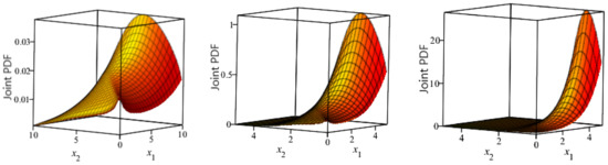
Figure 1. The surface plots of the joint probability density function (PDF) for ${\gamma }_1={\gamma }_2=$${\gamma }_3=0.3$and $a=0.1,$ $0.3$ and $0.5$, respectively.

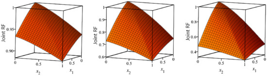
Figure 2. The surface plots of the joint reliability function (RF) for ${\gamma }_1={\gamma }_2=$${\gamma }_3=0.3$and $a=0.1,$ $0.3$ and $0.5$, respectively.

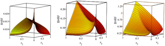
Figure 3. The surface plots of the bivariate hazard rate function (BHRF) for ${\gamma }_1={\gamma }_2=$${\gamma }_3=0.3$and $a=0.1,$ $0.3$ and $0.5$, respectively.

It is clear that the joint density has a long left tail as compared to its right tail. Moreover, the BBXEx distribution presents different shapes for the BHRF. Furthermore, the joint RF decreases for fixed values of ${\gamma }_1$, ${\gamma }_2$ and ${\gamma }_3$ with $a\to \infty$. Thus, this model can be used to discuss several phenomena in different fields. Reference [46] defined the local dependence function, say $\eta (x_1,x_2)$, in order to study the dependence between $X_1$ and $X_2$, where

$$\eta (x_1,x_2)=\frac{{\partial }^2}{\partial x_1\partial x_2}f(x_1,x_2).$$

(32)

If $\eta (x_1,x_2)$≥ 0, then $f(x_1,x_2)$ is a positivity of order two (PT2). Whereas if $\eta (x_1,x_2)$≤ 0, then $f(x_1,x_2)$ is a reverse rule of order two (RR2). Also, $f(x_1,x_2)$ is said to be PT2 (RR2) if $f(x_1,x_2)f(u,v)-f(x_1,v)f(u,x_2)\ge (\le )0$ for all $x_1\le u$ and $x_2\le v$. For the BBXEx distribution, it can be verified that $\eta (x_1,x_2)>0$, and then $X_1$ and $X_2$ are PT2. As a consequence,

• The linear correlation coefficient between $X_1$ and $X_2$ is always positive.
• The conditional hazard rate of $X_1|X_2=x_2$ is decreasing in $x_2.$
• The conditional hazard rate of $X_2|X_1=x_1$ is decreasing in $x_1.$

Recall, Equations (23) and (24), the correlation, skewness and kurtosis measures of the BBXEx distribution are listed in Table 1 for $(a,{\gamma }_1,{\gamma }_2,{\gamma }_3)=(1.5,0.6,{\gamma }_2,1.5)$.

Table 1. The correlation, skewness and kurtosis measures of the Burr X-exponential (BBXEx) (1.5,0.6,${\gamma }_2$,1.5) distribution.

Measures$\downarrow$ ${\gamma }_2⟶$	$0.2$	$0.5$	$0.8$	$1.1$	$1.4$	$1.7$	$2.0$	$2.3$	$2.6$	$2.9$
Correlation	$0.147$	$0.209$	$0.247$	$0.279$	$0.317$	$0.335$	$0.387$	$0.418$	$0.468$	$0.479$
Skewness	$1.879$	$1.314$	$1.149$	$1.045$	$0.687$	$0.564$	$0.001$	$0.045$	$0.059$	$0.098$
Kurtosis	$7.478$	$7.114$	$6.492$	$6.127$	$5.214$	$6.948$	$6.104$	$5.179$	$5.357$	$5.970$

From Table 1, it is observed that the value of correlation increases with ${\gamma }_2⟶\infty$ for fixed values of $a,{\gamma }_1$ and ${\gamma }_3$. Moreover, this distribution can be used to model skewed as well as symmetric data sets.

5. Estimation Based on Complete and Type-II Censored Samples

5.1. Maximum Likelihood Estimation

In this section, we compute the maximum likelihood estimation (MLE) for the unknown parameters $\mathsf{\Theta }=$($\mathit{\omega },{\gamma }_1,{\gamma }_2,{\gamma }_3$) based on complete and Type-II censored data. Suppose that $(x_{11},x_{21})$, $(x_{12},x_{22})$,…, $(x_{1n},x_{2n})$ are the observed values from the BBX-G family. We use the following notation $I_1=\{x_{1i}<x_{2i}\}$, $I_2=\{x_{1i}>x_{2i}\}$, $I_3=\{x_{1i}=x_{2i}=x_i\}$,$I=I_1\cup I_2\cup I_3$, $\left|I_1\right|=n_1,$$\left|I_2\right|=n_2,$$\left|I_3\right|=n_3,$ and $\left|I\right|=n_1+n_2+n_3=n.$ The total likelihood function for $\mathsf{\Theta }$ based on complete data can be defined as follows

$$l\left(\mathsf{\Theta }\right)={\displaystyle \prod _{i=1}^{n_1}}{f}_1(x_{1i},x_{2i}){\displaystyle \prod _{i=1}^{n_2}}{f}_2(x_{1i},x_{2i}){\displaystyle \prod _{i=1}^{n_3}}{f}_0\left(x_i\right).$$

(33)

Substituting Equation (5) into Equation (33), the log-likelihood function $L\left(\mathsf{\Theta }\right)$is given by

$$\begin{array}{cc}\hfill L\left(\mathsf{\Theta }\right)& =n_{1}ln\left(4{\gamma }_2\left({\gamma }_1+{\gamma }_3\right)\right)+{\displaystyle \sum _{i=1}^{n_1}}ln\left[g(x_{1i};\mathit{\omega })\right]+{\displaystyle \sum _{i=1}^{n_1}}ln\left[G(x_{1i};\mathit{\omega })\right]-3{\displaystyle \sum _{i=1}^{n_1}}ln\left[\overline{G}(x_{1i};\mathit{\omega })\right]\hfill \\ \hfill & -{\displaystyle \sum _{i=1}^{n_1}}{\left[\frac{G(x_{1i};\mathit{\omega })}{\overline{G}(x_{1i};\mathit{\omega })}\right]}^2+\left({\gamma }_1+{\gamma }_3-1\right){\displaystyle \sum _{i=1}^{n_1}}ln\left[1-e^{-{\left(\frac{G(x_{1i};\mathit{\omega })}{\overline{G}(x_{1i};\mathit{\omega })}\right)}^2}\right]+{\displaystyle \sum _{i=1}^{n_1}}ln\left[g(x_{2i};\mathit{\omega })\right]\hfill \\ \hfill & +{\displaystyle \sum _{i=1}^{n_1}}ln\left[G(x_{2i};\mathit{\omega })\right]-3{\displaystyle \sum _{i=1}^{n_1}}ln\left[\overline{G}(x_{2i};\mathit{\omega })\right]-{\displaystyle \sum _{i=1}^{n_1}}{\left[\frac{G(x_{2i};\mathit{\omega })}{\overline{G}(x_{2i};\mathit{\omega })}\right]}^2\hfill \\ \hfill & +\left({\gamma }_2-1\right){\displaystyle \sum _{i=1}^{n_1}}ln\left[1-e^{-{\left(\frac{G(x_{2i};\mathit{\omega })}{\overline{G}(x_{2i};\mathit{\omega })}\right)}^2}\right]+n_{2}ln\left(4{\gamma }_1({\gamma }_2+{\gamma }_3)\right)+{\displaystyle \sum _{i=1}^{n_2}}ln\left[g(x_{1i};\mathit{\omega })\right]\hfill \\ \hfill & +{\displaystyle \sum _{i=1}^{n_2}}ln\left[G(x_{1i};\mathit{\omega })\right]-3{\displaystyle \sum _{i=1}^{n_2}}ln\left[\overline{G}(x_{1i};\mathit{\omega })\right]-{\displaystyle \sum _{i=1}^{n_2}}{\left[\frac{G(x_{1i};\mathit{\omega })}{\overline{G}(x_{1i};\mathit{\omega })}\right]}^2\hfill \\ \hfill & +\left({\gamma }_1-1\right){\displaystyle \sum _{i=1}^{n_2}}ln\left[1-e^{-{\left(\frac{G(x_{1i};\mathit{\omega })}{\overline{G}(x_{1i};\mathit{\omega })}\right)}^2}\right]+{\displaystyle \sum _{i=1}^{n_2}}ln\left[g(x_{2i};\mathit{\omega })\right]+{\displaystyle \sum _{i=1}^{n_2}}ln\left[G(x_{2i};\mathit{\omega })\right]\hfill \\ \hfill & -3{\displaystyle \sum _{i=1}^{n_2}}ln\left[\overline{G}(x_{2i};\mathit{\omega })\right]-{\displaystyle \sum _{i=1}^{n_2}}{\left[\frac{G(x_{2i};\mathit{\omega })}{\overline{G}(x_{2i};\mathit{\omega })}\right]}^2+\left({\gamma }_2+{\gamma }_3-1\right){\displaystyle \sum _{i=1}^{n_2}}ln\left[1-e^{-{\left(\frac{G(x_{2i};\mathit{\omega })}{\overline{G}(x_{2i};\mathit{\omega })}\right)}^2}\right]\hfill \\ \hfill & +n_{3}ln\left[2{\gamma }_3\right]+{\displaystyle \sum _{i=1}^{n_3}}ln\left[g(x_i;\mathit{\omega })\right]+{\displaystyle \sum _{i=1}^{n_3}}ln\left[G(x_i;\mathit{\omega })\right]-3{\displaystyle \sum _{i=1}^{n_3}}ln\left[\overline{G}(x_i;\mathit{\omega })\right]\hfill \\ \hfill & -{\displaystyle \sum _{i=1}^{n_3}}{\left[\frac{G(x_i;\mathit{\omega })}{\overline{G}(x_i;\mathit{\omega })}\right]}^2+\left({\gamma }_1+{\gamma }_2+{\gamma }_3-1\right){\displaystyle \sum _{i=1}^{n_3}}ln\left(1-e^{-{\left(\frac{G(x_i;\mathit{\omega })}{\overline{G}(x_i;\mathit{\omega })}\right)}^2}\right).\hfill \end{array}$$

(34)

The first partial derivatives of Equation (34) with respect to ${\gamma }_1,{\gamma }_2,{\gamma }_3$ and ${\mathit{\omega }}_k$$(k=1,2,3,\dots )$ are

$$\begin{array}{cc}\hfill \frac{\partial L}{\partial {\gamma }_1}& =\frac{n_1}{{\gamma }_1+{\gamma }_3}+{\displaystyle \sum _{i=1}^{n_1}}ln\left[1-e^{-{\left(\frac{G(x_{1i};\mathit{\omega })}{\overline{G}(x_{1i};\mathit{\omega })}\right)}^2}\right]+\frac{n_2}{{\gamma }_1}+{\displaystyle \sum _{i=1}^{n_2}}ln\left[1-e^{-{\left(\frac{G(x_{1i};\mathit{\omega })}{\overline{G}(x_{1i};\mathit{\omega })}\right)}^2}\right]\hfill \\ \hfill & +{\displaystyle \sum _{i=1}^{n_3}}ln\left[1-e^{-{\left(\frac{G(x_i;\mathit{\omega })}{\overline{G}(x_i;\mathit{\omega })}\right)}^2}\right],\hfill \end{array}$$

(35)

$$\begin{array}{cc}\hfill \frac{\partial L}{\partial {\gamma }_2}& =\frac{n_1}{{\gamma }_2}+{\displaystyle \sum _{i=1}^{n_1}}ln\left[1-e^{-{\left(\frac{G(x_{2i};\mathit{\omega })}{\overline{G}(x_{2i};\mathit{\omega })}\right)}^2}\right]+\frac{n_2}{{\gamma }_2+{\gamma }_3}+{\displaystyle \sum _{i=1}^{n_2}}ln\left[1-e^{-{\left(\frac{G(x_{2i};\mathit{\omega })}{\overline{G}(x_{2i};\mathit{\omega })}\right)}^2}\right]\hfill \\ \hfill & +{\displaystyle \sum _{i=1}^{n_3}}ln\left[1-e^{-{\left(\frac{G(x_i;\mathit{\omega })}{\overline{G}(x_i;\mathit{\omega })}\right)}^2}\right],\hfill \end{array}$$

(36)

$$\begin{array}{cc}\hfill \frac{\partial L}{\partial {\gamma }_3}& =\frac{n_1}{{\gamma }_1+{\gamma }_3}+{\displaystyle \sum _{i=1}^{n_1}}ln\left[1-e^{-{\left(\frac{G(x_{1i};\mathit{\omega })}{\overline{G}(x_{1i};\mathit{\omega })}\right)}^2}\right]+\frac{n_2}{{\gamma }_2+{\gamma }_3}+{\displaystyle \sum _{i=1}^{n_2}}ln\left[1-e^{-{\left(\frac{G(x_{2i};\mathit{\omega })}{\overline{G}(x_{2i};\mathit{\omega })}\right)}^2}\right]\hfill \\ \hfill & +\frac{n_3}{{\gamma }_3}+{\displaystyle \sum _{i=1}^{n_3}}ln\left[1-e^{-{\left(\frac{G(x_i;\mathit{\omega })}{\overline{G}(x_i;\mathit{\omega })}\right)}^2}\right]\hfill \end{array}$$

(37)

and

$$\begin{array}{cc}\hfill \frac{\partial L}{\partial {\mathit{\omega }}_k}& ={\displaystyle \sum _{i=1}^{n_1}}\frac{{\left[g(x_{1i};\mathit{\omega })\right]}^{\left({\mathit{\omega }}_k\right)}}{g(x_{1i};\mathit{\omega })}+{\displaystyle \sum _{i=1}^{n_1}}\frac{{\left[G(x_{1i};\mathit{\omega })\right]}^{\left({\mathit{\omega }}_k\right)}}{G(x_{1i};\mathit{\omega })}-2{\displaystyle \sum _{i=1}^{n_1}}\frac{G(x_{1i};\mathit{\omega })}{\overline{G}(x_{1i};\mathit{\omega })}{\left[\frac{G(x_{1i};\mathit{\omega })}{\overline{G}(x_{1i};\mathit{\omega })}\right]}^{\left({\mathit{\omega }}_k\right)}\hfill \\ \hfill & -3{\displaystyle \sum _{i=1}^{n_1}}\frac{{\left[\overline{G}(x_{1i};\mathit{\omega })\right]}^{\left({\mathit{\omega }}_k\right)}}{\overline{G}(x_{1i};\mathit{\omega })}+2({\gamma }_1+{\gamma }_3-1){\displaystyle \sum _{i=1}^{n_1}}\frac{G(x_{1i};\mathit{\omega })}{\overline{G}(x_{1i};\mathit{\omega })}{\left[\frac{G(x_{1i};\mathit{\omega })}{\overline{G}(x_{1i};\mathit{\omega })}\right]}^{\left({\mathit{\omega }}_k\right)}\times \hfill \\ \hfill & {\left(e^{{\left(\frac{G(x_i;\mathit{\omega })}{\overline{G}(x_i;\mathit{\omega })}\right)}^2}-1\right)}^{-1}+{\displaystyle \sum _{i=1}^{n_1}}\frac{{\left[G(x_{2i};\mathit{\omega })\right]}^{\left({\mathit{\omega }}_k\right)}}{G(x_{2i};\mathit{\omega })}-2{\displaystyle \sum _{i=1}^{n_1}}\frac{G(x_{2i};\mathit{\omega })}{\overline{G}(x_{2i};\mathit{\omega })}{\left[\frac{G(x_{2i};\mathit{\omega })}{\overline{G}(x_{2i};\mathit{\omega })}\right]}^{\left({\mathit{\omega }}_k\right)}\hfill \\ \hfill & +{\displaystyle \sum _{i=1}^{n_1}}\frac{{\left[g(x_{2i};\mathit{\omega })\right]}^{\left({\mathit{\omega }}_k\right)}}{g(x_{2i};\mathit{\omega })}-3{\displaystyle \sum _{i=1}^{n_1}}\frac{{\left[\overline{G}(x_{2i};\mathit{\omega })\right]}^{\left({\mathit{\omega }}_k\right)}}{\overline{G}(x_{2i};\mathit{\omega })}+{\displaystyle \sum _{i=1}^{n_2}}\frac{{\left[g(x_{1i};\mathit{\omega })\right]}^{\left({\mathit{\omega }}_k\right)}}{g(x_{1i};\mathit{\omega })}\hfill \\ \hfill & +2\left({\gamma }_2-1\right){\displaystyle \sum _{i=1}^{n_1}}\frac{G(x_{2i};\mathit{\omega })}{\overline{G}(x_{2i};\mathit{\omega })}{\left[\frac{G(x_{2i};\mathit{\omega })}{\overline{G}(x_{2i};\mathit{\omega })}\right]}^{\left({\mathit{\omega }}_k\right)}{\left(e^{{\left(\frac{G(x_{2i};\mathit{\omega })}{\overline{G}(x_{2i};\mathit{\omega })}\right)}^2}-1\right)}^{-1}\hfill \\ \hfill & +{\displaystyle \sum _{i=1}^{n_2}}\frac{{\left[G(x_{1i};\mathit{\omega })\right]}^{\left({\mathit{\omega }}_k\right)}}{G(x_{1i};\mathit{\omega })}-3{\displaystyle \sum _{i=1}^{n_2}}\frac{{\left[\overline{G}(x_{1i};\mathit{\omega })\right]}^{\left({\mathit{\omega }}_k\right)}}{\overline{G}(x_{1i};\mathit{\omega })}+{\displaystyle \sum _{i=1}^{n_2}}\frac{{\left[g(x_{2i};\mathit{\omega })\right]}^{\left({\mathit{\omega }}_k\right)}}{g(x_{2i};\mathit{\omega })}\hfill \\ \hfill & -2{\displaystyle \sum _{i=1}^{n_2}}\frac{G(x_{1i};\mathit{\omega })}{\overline{G}(x_{1i};\mathit{\omega })}{\left[\frac{G(x_{1i};\mathit{\omega })}{\overline{G}(x_{1i};\mathit{\omega })}\right]}^{\left({\mathit{\omega }}_k\right)-1}+{\displaystyle \sum _{i=1}^{n_2}}\frac{{\left[G(x_{2i};\mathit{\omega })\right]}^{\left({\mathit{\omega }}_k\right)}}{G(x_{2i};\mathit{\omega })}\hfill \\ \hfill & +2\left({\gamma }_1-1\right){\displaystyle \sum _{i=1}^{n_1}}\frac{G(x_{1i};\mathit{\omega })}{\overline{G}(x_{1i};\mathit{\omega })}{\left[\frac{G(x_{1i};\mathit{\omega })}{\overline{G}(x_{1i};\mathit{\omega })}\right]}^{\left({\mathit{\omega }}_k\right)}\left(e^{{\left(\frac{G(x_i;\mathit{\omega })}{\overline{G}(x_i;\mathit{\omega })}\right)}^2}-1\right)\hfill \\ \hfill & -3{\displaystyle \sum _{i=1}^{n_2}}\frac{{\left[\overline{G}(x_{2i};\mathit{\omega })\right]}^{\left({\mathit{\omega }}_k\right)}}{\overline{G}(x_{2i};\mathit{\omega })}-2{\displaystyle \sum _{i=1}^{n_2}}\frac{G(x_{2i};\mathit{\omega })}{\overline{G}(x_{2i};\mathit{\omega })}{\left[\frac{G(x_{2i};\mathit{\omega })}{\overline{G}(x_{2i};\mathit{\omega })}\right]}^{\left({\mathit{\omega }}_k\right)}\hfill \\ \hfill & +2\left({\gamma }_2+{\gamma }_3-1\right){\displaystyle \sum _{i=1}^{n_2}}\frac{G(x_{2i};\mathit{\omega })}{\overline{G}(x_{2i};\mathit{\omega })}{\left[\frac{G(x_{2i};\mathit{\omega })}{\overline{G}(x_{2i};\mathit{\omega })}\right]}^{\left({\mathit{\omega }}_k\right)}{\left(e^{{\left(\frac{G(x_{2i};\mathit{\omega })}{\overline{G}(x_{2i};\mathit{\omega })}\right)}^2}-1\right)}^{-1}\hfill \\ \hfill & +{\displaystyle \sum _{i=1}^{n_2}}\frac{g^{\left({\mathit{\omega }}_k\right)}(x_{2i};\mathit{\omega })}{g(x_{2i};\mathit{\omega })}-2{\displaystyle \sum _{i=1}^{n_2}}\frac{{\left(\overline{G}(x_{2i};\mathit{\omega })\right)}^{\left({\mathit{\omega }}_k\right)}}{\overline{G}(x_{2i};\mathit{\omega })}-\alpha {\displaystyle \sum _{i=1}^{n_2}}{\left(\frac{G(x_{2i};\mathit{\omega })}{\overline{G}(x_{2i};\mathit{\omega })}\right)}^{\left({\mathit{\omega }}_k\right)}\hfill \\ \hfill & +{\displaystyle \sum _{i=1}^{n_3}}\frac{{\left[g(x_i;\mathit{\omega })\right]}^{\left({\mathit{\omega }}_k\right)}}{g(x_i;\mathit{\omega })}+{\displaystyle \sum _{i=1}^{n_3}}\frac{{\left[G(x_i;\mathit{\omega })\right]}^{\left({\mathit{\omega }}_k\right)}}{G(x_i;\mathit{\omega })}-3{\displaystyle \sum _{i=1}^{n_3}}\frac{{\left[\overline{G}(x_i;\mathit{\omega })\right]}^{\left({\mathit{\omega }}_k\right)}}{\overline{G}(x_i;\mathit{\omega })}\hfill \\ \hfill & +2\left({\gamma }_1+{\gamma }_2+{\gamma }_3-1\right){\displaystyle \sum _{i=1}^{n_3}}\frac{G(x_i;\mathit{\omega })}{\overline{G}(x_i;\mathit{\omega })}{\left[\frac{G(x_i;\mathit{\omega })}{\overline{G}(x_i;\mathit{\omega })}\right]}^{\left({\mathit{\omega }}_k\right)}{\left(e^{{\left(\frac{G(x_i;\mathit{\omega })}{\overline{G}(x_i;\mathit{\omega })}\right)}^2}-1\right)}^{-1}\hfill \\ \hfill & -2{\displaystyle \sum _{i=1}^{n_3}}\frac{G(x_i;\mathit{\omega })}{\overline{G}(x_i;\mathit{\omega })}{\left[\frac{G(x_i;\mathit{\omega })}{\overline{G}(x_i;\mathit{\omega })}\right]}^{\left({\mathit{\omega }}_k\right)}.\hfill \end{array}$$

(38)

where ${\left[U(.)\right]}^{\left(\mathit{\omega }\right)}$ means the derivative of the function U $(.)$ with respect to $\mathit{\omega }$. By equating the Equations (35)–(38) by zeros, we get the non-linear normal equations. The likelihood function for the bivariate distribution based on Type-II censored data can be written as follows

$$l^{*}\left(\mathsf{\Theta }\right)=\frac{n!}{\left(n-r\right)!}{(1-F\left(x_{1_{i:n}}\right))}^{n-r}{\displaystyle \prod _{i=1}^r}{f}_{X_1,X_2}\left(x_{1_{i:n}},x_{2\left[{}_{i:n}\right]}\right),$$

(39)

(see [47]). The log-likelihood function $L^{*}\left(\mathsf{\Theta }\right)$can be expressed as follows

$$L^{*}\left(\mathsf{\Theta }\right)=ln\left(\frac{n!}{\left(n-r\right)!}\right)+\left(n-r\right)ln\left(1-F\left(x_{1_{i:n}}\right)\right)+\sum _{i=1}^{r}ln\left(f_{X_1,X_2}\left(x_{1_{i:n}},x_{2\left[{}_{i:n}\right]}\right)\right).$$

(40)

Substituting from Equations (5) and (7) into Equation (40), and then differentiation the result equation with respect to ${\gamma }_1,{\gamma }_2,{\gamma }_3$ and ${\mathit{\omega }}_k$$(k=1,2,3,\dots ).$ The MLEs of the parameters can be obtained by solving the normal equations simultaneously.

5.2. Bayesian Estimation

In this section, we consider the Bayesian estimation under the assumption that the non-negative parameters of $\mathit{\omega },{\gamma }_1,{\gamma }_2$ and ${\gamma }_3$ are independently distributed with gamma prior distribution where $\mathit{\omega }=({\omega }_1,{\omega }_2,\dots ,{\omega }_k)$. So, $\pi \left({\omega }_j\right)\propto {\omega }_j^{{\mathsf{\Omega }}_j-1}{e}^{-{\mathsf{\Psi }}_j{\omega }_j};j=1,\dots ,k$ and $\pi \left({\gamma }_l\right)\propto {\gamma }_l^{{\mathsf{\Omega }}_l-1}{e}^{-{\mathsf{\Psi }}_l{\gamma }_l};l=1,2,3.$ All the hyper parameters ${\mathsf{\Omega }}_j$, ${\mathsf{\Psi }}_j,$${\mathsf{\Omega }}_l$ and ${\mathsf{\Psi }}_l$are assumed to be known and non-negative. The joint prior density of unknown parameters $\mathit{\omega },{\gamma }_1,{\gamma }_2$ and ${\gamma }_3$ can be written as follows

$$\pi (\mathit{\omega },{\gamma }_1,{\gamma }_2,{\gamma }_3)\propto \left({\displaystyle \prod _{j=1}^k}{\omega }_j^{{\mathsf{\Omega }}_j-1}{e}^{-{\mathsf{\Psi }}_j{\omega }_j}\right)\left({\displaystyle \prod _{l=1}^3}{\gamma }_l^{{\mathsf{\Omega }}_l-1}{e}^{-{\mathsf{\Psi }}_l{\gamma }_l}\right).$$

(41)

Combining Equations (34) and (41), the posterior density of $\mathit{\omega },{\gamma }_1,{\gamma }_2$ and ${\gamma }_3$ can be expressed as follows

$$\dot{\pi }(\mathit{\omega },{\gamma }_1,{\gamma }_2,{\gamma }_3|X_1,X_2)=\frac{l(\mathit{\omega },{\gamma }_1,{\gamma }_2,{\gamma }_3|X_1,X_2)\pi (\mathit{\omega },{\gamma }_1,{\gamma }_2,{\gamma }_3)}{{\int }_{\mathit{\omega }}{\int }_{{\gamma }_1}{\int }_{{\gamma }_2}{\int }_{{\gamma }_3}l(\mathit{\omega },{\gamma }_1,{\gamma }_2,{\gamma }_3|X_1,X_2)\pi (\mathit{\omega },{\gamma }_1,{\gamma }_2,{\gamma }_3)d{\gamma }_{3}d{\gamma }_{2}d{\gamma }_{1}d\mathit{\omega }}.$$

(42)

Equation (42) can be expressed in a simple form as follows

$$\dot{\pi }(\mathit{\omega },{\gamma }_1,{\gamma }_2,{\gamma }_3|X_1,X_2)\propto l(\mathit{\omega },{\gamma }_1,{\gamma }_2,{\gamma }_3|X_1,X_2)\pi (\mathit{\omega },{\gamma }_1,{\gamma }_2,{\gamma }_3).$$

(43)

Thus, the Bayesian estimators of the parameters $\mathit{\omega }$ and ${\gamma }_l$ under square error loss function can be calculated through the following equations as follows

$$\widehat{{\omega }_j}\propto \underset{{\omega }_j}{\int }{\omega }_j\dot{\pi }(\mathit{\omega },{\gamma }_1,{\gamma }_2,{\gamma }_3|X_1,X_2)d{\omega }_j,$$

(44)

and

$$\widehat{{\gamma }_l}\propto \underset{0}{\overset{\infty }{\int }}{\gamma }_l\dot{\pi }(\mathit{\omega },{\gamma }_1,{\gamma }_2,{\gamma }_3|X_1,X_2)d{\gamma }_l,$$

(45)

respectively, where $j=1,\dots ,k$ and $l=1,2,3$. Generally, the ratio of $k+l$ integrals given by Equations (44) and (45) cannot be obtained in a closed form, so we may use the Markov chain Monte Carlo (MCMC) technique. In MCMC methods, we estimate the posterior distribution and the intractable integrals using simulated samples from the posterior distribution. We can use Gibbs sampling and the Metropolis–Hastings (M-H) algorithm as a MCMC technique. This algorithm was first introduced in [48,49]. Similarly to acceptance–rejection sampling, the M-H algorithm consider that to each iteration of the algorithm, a candidate value can be generated from a proposal distribution. So, the candidate value is accepted according to an adequate acceptance probability. This procedure guarantees the convergence of the Markov chain for the target density. For more details regarding the implementation of M-H algorithm, the readers may refer to [50,51,52].

Regarding to the Type-II censored data, Equation (39) can be used instead of Equation (33) to get the Bayes estimates of the unknown parameters $\mathit{\omega },{\gamma }_1,{\gamma }_2$ and ${\gamma }_3$. At the end of this section, we can conclude that the advantage of using the MCMC method over the MLE method is that we can always obtain a reasonable interval estimate of the parameters by constructing the probability intervals based on empirical posterior distribution. This is often unavailable in MLE.

5.3. Bootstrap Confidence Interval

5.3.1. Percentile Bootstrap Confidence Interval

The following algorithm shows how to calculate the percentile bootstrap confidence interval (P-BCI) for the model parameters:

• Compute the MLE of ${\mathsf{\Theta }}_k$ where $k=$length $\left(\mathsf{\Theta }\right)$ for BBXEx model.
• Generate the bootstrap samples using ${\mathsf{\Theta }}_k$ to obtain the bootstrap estimate of ${\mathsf{\Theta }}_k,$ say ${\widehat{\mathsf{\Theta }}}_k^b,$ using the bootstrap sample.
• Repeat step 2 T times to have $({\widehat{\mathsf{\Theta }}}_k^{b\left(1\right)},{\widehat{\mathsf{\Theta }}}_k^{b\left(2\right)},\dots ,{\widehat{\mathsf{\Theta }}}_k^{b\left(T\right)})$.
• Arrange $({\widehat{\mathsf{\Theta }}}_k^{b\left(1\right)},{\widehat{\mathsf{\Theta }}}_k^{b\left(2\right)},\dots ,{\widehat{\mathsf{\Theta }}}_k^{b\left(T\right)})$ in ascending order as $({\widehat{\mathsf{\Theta }}}_k^{b\left[1\right]},{\widehat{\mathsf{\Theta }}}_k^{b\left[2\right]},\dots ,{\widehat{\mathsf{\Theta }}}_k^{b\left[T\right]})$.
• A two side $100(1-\alpha )\%$ P-BCI for the unknown parameters ${\mathsf{\Theta }}_k$ is given by $\left[{\widehat{\mathsf{\Theta }}}_k^{b\left[T\right]\alpha /2},{\widehat{\mathsf{\Theta }}}_k^{b\left[T\right](1-\alpha /2)}\right]$.

5.3.2. Percentile Bootstrap-t Confidence Interval

The following algorithm shows how to calculate the percentile bootstrap-t confidence interval (B-TCI) for the model parameters:

• Same as steps 1 and 2 in P-BCI.
• Compute the $t-$statistic of ${\mathsf{\Theta }}_k$ as $({\widehat{\mathsf{\Theta }}}_k^b-{\widehat{\mathsf{\Theta }}}_k)/\sqrt{V\left({\widehat{\mathsf{\Theta }}}_k^b\right)}$ where $V\left({\widehat{\mathsf{\Theta }}}_k^b\right)$ is asymptotic variances of ${\widehat{\mathsf{\Theta }}}_k^b$ and it can be obtained using the Fisher information matrix.
• Repeat steps 2 and 3 T times and obtain $t-$statistic${}^{\left(1\right)},t-$statistic${}^{\left(2\right)},\dots ,t-$statistic${}^{\left(T\right)}$.
• Arrange $t-$statistic${}^{\left(1\right)},t-$statistic${}^{\left(2\right)},\dots ,t-$statistic${}^{\left(T\right)}$ in ascending order as $t-$statistic${}^{\left[1\right]},t-$statistic${}^{\left[2\right]},\dots ,t-$statistic${}^{\left[T\right]}$.
• A two side $100(1-\alpha )\%$ B-TCI for the unknown parameters ${\mathsf{\Theta }}_k$ is given by

  $$\left[{\widehat{\mathsf{\Theta }}}_k+t-{\mathrm{statistic}}^{\left[T\right]\alpha /2}\sqrt[2]{V\left({\widehat{\mathsf{\Theta }}}_k^b\right)},{\widehat{\mathsf{\Theta }}}_k+t-{\mathrm{statistic}}^{\left[T\right](1-\alpha /2)}\sqrt[2]{V\left({\widehat{\mathsf{\Theta }}}_k^b\right)}\right].$$

6. Simulation Based on Complete and Type-II Censored Samples

6.1. Simulation Results Based on Complete Data

In this section, the MLE, Bayesian estimation (BSE) and bootstrap confidence interval (BCI) methods are used to estimate the parameters $a,{\gamma }_1,{\gamma }_2$ and ${\gamma }_3$ of the BBXEx distribution by using different sample sizes $n=[$50, 100, 150, 200, 300] from $N=$1000 replications. The population parameters are generated using the software R package. For more details around the R package, see [50,51]. This study presents an assessment of the properties for both MLE and BSE in terms of bias and mean square error (MSE) as well as the BCI for the parameters. The following algorithm shows how to generate data from the BBXEx distribution.

• Generate $A_1$, $A_2$and $A_3$ from $A(0,1).$
• Compute $U_i=Q_G\left({\left({\left[-log\left(1-A_i^{\frac{1}{{\gamma }_i}}\right)\right]}^{-0.5}+1\right)}^{-1}\right);i=1,2,3.$
• Obtain $X_1=max\{U_1,U_3\}$and$X_2=max\{U_2,U_3\}.$

The MLEs and BSEs as well as the BCI values are listed in Table 2 for the BBXEx distribution when $(a,{\gamma }_1,{\gamma }_2,{\gamma }_3)=(5,0.7,0.8,0.9)$ based on complete data.

Table 2. Estimation summaries for the BBXEx distribution based on complete data.

		MLE		BSE		BCI
$\mathit{n}$	Parameter	Bias	MSE	Bias	MSE	Average CI	B-TCI	P-BCI
50	$a=5$	$0.0266$	$0.0480$	$0.0177$	$0.0380$	$0.8532$	$0.0272$	$0.0269$
	${\gamma }_1=0.7$	$0.1378$	$0.0663$	$0.0391$	$0.0224$	$0.8532$	$0.0270$	$0.0276$
	${\gamma }_2=0.8$	$-0.276$	$0.1250$	$-0.057$	$0.0261$	$5.7491$	$0.1781$	$0.1778$
	${\gamma }_3=0.9$	$0.0914$	$0.0693$	$0.0231$	$0.0269$	$5.0284$	$0.1610$	$0.1679$
100	$a=5$	$0.0143$	$0.0228$	$0.0152$	$0.0207$	$0.5896$	$0.0186$	$0.0195$
	${\gamma }_1=0.7$	$0.1123$	$0.0348$	$0.0389$	$0.0138$	$0.5840$	$0.0184$	$0.0181$
	${\gamma }_2=0.8$	$-0.156$	$0.1211$	$-0.050$	$0.0211$	$3.2938$	$0.1026$	$0.1040$
	${\gamma }_3=0.9$	$0.0779$	$0.0554$	$0.0210$	$0.0214$	$2.9020$	$0.0913$	$0.0900$
150	$a=5$	$0.0140$	$0.0158$	$0.0144$	$0.0157$	$0.4882$	$0.0156$	$0.0153$
	${\gamma }_1=0.7$	$0.1106$	$0.0284$	$0.0293$	$0.0131$	$0.4770$	$0.0150$	$0.0154$
	${\gamma }_2=0.8$	$-0.123$	$0.0309$	$-0.047$	$0.0173$	$2.0961$	$0.0662$	$0.0655$
	${\gamma }_3=0.9$	$0.0439$	$0.0208$	$0.0177$	$0.0145$	$1.7794$	$0.0560$	$0.0557$
200	$a=5$	$0.0108$	$0.0103$	$0.0114$	$0.0102$	$0.3958$	$0.0125$	$0.0125$
	${\gamma }_1=0.7$	$0.1101$	$0.0230$	$0.0178$	$0.0115$	$0.4052$	$0.0133$	$0.0131$
	${\gamma }_2=0.8$	$-0.088$	$0.0165$	$-0.033$	$0.0150$	$0.3645$	$0.0115$	$0.0113$
	${\gamma }_3=0.9$	$0.0089$	$0.0096$	$0.0108$	$0.0075$	$0.3836$	$0.0126$	$0.0123$
300	$a=5$	$0.0052$	$0.0078$	$0.0083$	$0.0073$	$0.3448$	$0.0110$	$0.0108$
	${\gamma }_1=0.7$	$0.1041$	$0.0179$	$0.0097$	$0.0108$	$0.3300$	$0.0105$	$0.0108$
	${\gamma }_2=0.8$	$-0.078$	$0.0153$	$-0.013$	$0.0121$	$0.2960$	$0.0095$	$0.0094$
	${\gamma }_3=0.9$	$0.0036$	$0.0063$	$0.0045$	$0.0061$	$0.3100$	$0.0098$	$0.0097$

From Table 2, the following observations can be noted:

• The MSEs for the MLE and BSE always decrease to zero when n grows.
• The magnitude of bias in general always close to zero when n grows.
• Based on the MSE, the performance of the BSE method is better than the MLE method.
• The confidence in the results increases as the sample size increases where the BCI decreases when n grows.

6.2. Simulation Results Based on Type-II Censored Samples

The following algorithm shows how to generate Type-II censored bivariate samples from the BBXEx distribution:

• Generate $A_1$, $A_2$and $A_3$ from $A(0,1).$
• Compute $U_i=Q_G\left({\left({\left[-log\left(1-A_i^{\frac{1}{{\gamma }_i}}\right)\right]}^{-0.5}+1\right)}^{-1}\right);i=1,2,3.$
• Repeat steps 1 and 2 n times to obtain ($X_{1_i},X_{2_i}$), $i=1,2,\dots ,n.$
• Arrange $X_{1_i};i=1,2,\dots ,n$ in ascending order to obtain $X_{1_{1:n}}\le X_{1_{2:n}}\le \dots \le X_{1_{n:n}}$ and form $(X_{1_{i:n}},X_{2_{[i:n]}});$$i=1,2,\dots ,n,$ where $X_{2_{[i:n]}}$ is the $X_2$ sample value associated with $X_{1_i};i=1,2,\dots ,n.$
• Type-II censored data are obtained by keeping the first r pairs of ordered observations $(X_{1_{j:n}},X_{2_{[j:n]}});$$i=1,2,\dots ,n$ and dropping the remaining $n-r$ observations.

The MLEs and BSEs as well as the BCI values are reported in Table 3 and Table 4 for the BBXEx distribution when $(a,{\gamma }_1,{\gamma }_2,{\gamma }_3)=(5,0.7,0.8,0.9)$ based on Type-II censored data for different sample sizes $n=100$ and 200, respectively.

Table 3. Estimation summaries for the BBXEx model based on Type-II censored data at n = 100.

			MLE		BSE		BCI
$\mathit{n}$	$\mathit{r}$	Parameter	Bias	MSE	Bias	MSE	Average CI	B-TCI	P-BCI
100	30	$a=5$	$0.1185$	$0.1347$	$-0.1841$	$0.0643$	$1.3632$	$0.0614$	$0.0623$
		${\gamma }_1=0.7$	$0.2422$	$0.1841$	$0.3428$	$0.2183$	$1.2178$	$0.0547$	$0.0568$
		${\gamma }_2=0.8$	$0.0315$	$0.0441$	$-0.0550$	$0.0302$	$0.8149$	$0.0363$	$0.0360$
		${\gamma }_3=0.9$	$-0.3307$	$0.1085$	$-0.4699$	$0.2348$	$0.4065$	$0.0179$	$0.0178$
	50	$a=5$	$0.0750$	$0.0638$	$-0.1323$	$0.0636$	$0.9463$	$0.0415$	$0.0416$
		${\gamma }_1=0.7$	$0.1355$	$0.1816$	$0.2700$	$0.1565$	$0.8824$	$0.0387$	$0.0396$
		${\gamma }_2=0.8$	$0.0139$	$0.0287$	$-0.0484$	$0.0231$	$0.6626$	$0.0289$	$0.0293$
		${\gamma }_3=0.9$	$-0.1658$	$0.0302$	$-0.3495$	$0.1356$	$0.4013$	$0.0160$	$0.0165$
	70	$a=5$	$0.0253$	$0.0278$	$-0.0360$	$0.0237$	$0.6464$	$0.0296$	$0.0233$
		${\gamma }_1=0.7$	$0.0850$	$0.1781$	$0.1137$	$0.0597$	$0.6782$	$0.0305$	$0.0313$
		${\gamma }_2=0.8$	$0.0044$	$0.0218$	$-0.0384$	$0.0172$	$0.5638$	$0.0239$	$0.0241$
		${\gamma }_3=0.9$	$-0.0935$	$0.0134$	$-0.1478$	$0.0352$	$0.4001$	$0.0125$	$0.0126$

Table 4. Estimation summaries for the BBXEx model based on Type-II censored data at n = 200.

			MLE		BSE		BCI
$\mathit{n}$	$\mathit{r}$	Parameter	Bias	MSE	Bias	MSE	Average CI	B-TCI	P-BCI
200	70	$a=5$	$0.0657$	$0.0501$	$-0.1284$	$0.0537$	$0.8396$	$0.0373$	$0.0374$
		${\gamma }_1=0.7$	$0.1472$	$0.1508$	$0.1961$	$0.3737$	$0.7129$	$0.0309$	$0.0314$
		${\gamma }_2=0.8$	$-0.0108$	$0.0201$	$-0.0567$	$0.0173$	$0.5543$	$0.0251$	$0.0248$
		${\gamma }_3=0.9$	$-0.1941$	$0.1572$	$-0.1183$	$0.2737$	$0.2573$	$0.0116$	$0.0120$
	100	$a=5$	$0.0424$	$0.0274$	$-0.0687$	$0.0290$	$0.6284$	$0.0275$	$0.0288$
		${\gamma }_1=0.7$	$0.1043$	$0.1180$	$0.1149$	$0.2803$	$0.5821$	$0.0266$	$0.0271$
		${\gamma }_2=0.8$	$-0.0130$	$0.0137$	$-0.0456$	$0.0128$	$0.4515$	$0.0199$	$0.0198$
		${\gamma }_3=0.9$	$-0.1774$	$0.1329$	$-0.1073$	$0.1797$	$0.2550$	$0.0110$	$0.0119$
	150	$a=5$	$0.0230$	$0.0161$	$-0.0185$	$0.0148$	$0.4891$	$0.0219$	$0.0222$
		${\gamma }_1=0.7$	$0.0119$	$0.0229$	$0.1014$	$0.1179$	$0.4651$	$0.0210$	$0.0204$
		${\gamma }_2=0.8$	$-0.0010$	$0.0116$	$-0.0268$	$0.0120$	$0.3886$	$0.0174$	$0.0174$
		${\gamma }_3=0.9$	$-0.1440$	$0.0662$	$-0.0877$	$0.0540$	$0.2504$	$0.0105$	$0.0109$

Based on the simulation results, it is clear that:

• The biases and MSEs of both MLEs and BSEs decrease when the sampling r increases for a fixed sample size $n.$
• The MLE and BSE methods provide a fit for estimating the model parameters.
• The ACI, BT and BP decrease when the sampling r increases for a fixed sample size n. So, confidence in the results increases as the sample size increases where the results approaching the real average.

7. Real Data

In this section, we illustrate the empirical importance of the BBXEx distribution using two applications to real data. The fitted distributions are compared using some criteria, namely, the maximized log-likelihood (L), Akaike information criterion (AIC), corrected AIC (CAIC), Bayesian IC (BIC) and Hannan–Quinn IC (HQIC); in addition to the Kolmogorov–Smirnov (KS) statistic and its p-value for the marginals. For more details regarding these criteria, see [53,54,55,56].

7.1. Data Set I: Football Data

Here, consider the data obtained by [57], which represent football (soccer) data. This data describes the games where at least one kick goal scored by any team has been considered, and the home team must have scored at least one goal. This data was analyzed by several authors, see for example, [24,25,58,59]. We consider the BBXEx model to analyze this data, comparing with other famous bivariate models, such as bivariate generalized exponential (BGEx), bivariate exponential (BEx), bivariate Gumbel exponential (BGuEx), bivariate generalized linear failure rate (BGLFR), bivariate Weibull (BW), bivariate exponentiated Weibull (BEW), bivariate generalized power Weibull (BGPW) and bivariate Gompertz (BGz) distributions. Figure 4 shows that the scatter plot for data set I.

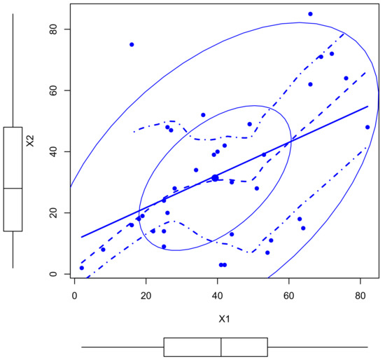
Figure 4. The scatter plot for data set I.

We fit at first the marginals $X_1$, $X_2$ and $min(X_1,X_2)$ separately on the UEFA Champion’s League data. The MLEs of the parameters ($\gamma ,a$) of the corresponding Burr X-exponential (BXEx) model for $X_1$, $X_2$ and $min(X_1,X_2)$ are ($0.724,0.013$), ($0.445,0.012$) and ($0.459,0.014$), respectively with standard error (STER) ($0.137,0.001$), ($0.080,0.001$) and ($0.083,0.001$). The $-L$, KS distance and its p-value for the marginals are listed in Table 5.

Table 5. The log-likelihood (L), Kolmogorov–Smirnov (KS) and p-values for the marginals using data set I.

	${\mathit{X}}_1$			${\mathit{X}}_2$			$min({\mathit{X}}_1,{\mathit{X}}_2)$
Model	$-\mathit{L}$	KS	p-Value	$-\mathit{L}$	KS	p-Value	$-\mathit{L}$	KS	p-Value
BXEx	$161.879$	$0.092$	$0.912$	$162.739$	$0.112$	$0.743$	$158.322$	$0.109$	$0.769$

It is clear that the BXEx model fits the data for the marginals. The fitted PDF, estimated CDF and PP plots displayed in Figure 5, Figure 6 and Figure 7 which support our results in Table 5. The fitted PDF, estimated CDF and probability–probability (PP) plots displayed in Figure 5, Figure 6 and Figure 7 which support our results in Table 5.

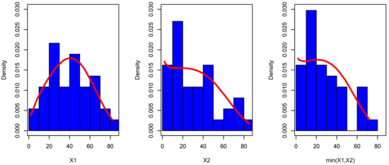
Figure 5. The fitted PDF for $X_1$, $X_2$ and $min(X_1,X_2)$ for data set I.

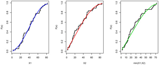
Figure 6. The estimated cumulative distribution function (CDF) for $X_1$, $X_2$ and $min(X_1,X_2)$ for data set I.

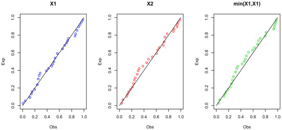
Figure 7. The probability–probability (PP) plots for $X_1$, $X_2$ and $min(X_1,X_2)$ for data set I.

From Figure 5, Figure 6 and Figure 7, it is quite apparent that the marginals can be used to discuss this data. Therefore, the BBXEx model may be used for this purpose. Now, we fit the BBXEx model on this data. In the enclosed Table 6, we provide the MLEs with its corresponding standard error (STER), $-L$, AIC, CAIC, BIC and HQIC values for tested distributions.

Table 6. The maximum likelihood estimation (MLE) and goodness-of-fit measures for data set I.

		Model
Statistic		BBXEx	BGEx	BEx	BGuEx	BGLFR	BW	BEW	BGPW	BGz
$\widehat{{\gamma }_1}$	MLE	$0.385$	$1.553$	$0.012$	$2.678$	$0.452$	$0.397$	$1.227$	$3.229$	$0.033$
	STER	$0.093$	$0.437$	$0.772$	$0.760$	$0.094$	$0.063$	$0.772$	$4.252$	$0.001$
$\widehat{{\gamma }_2}$	MLE	$0.136$	$0.499$	$0.014$	$0.962$	$0.156$	$0.274$	$0.382$	$1.983$	$0.002$
	STER	$0.052$	$0.198$	$0.356$	$0.367$	$0.055$	$0.066$	$0.356$	$2.580$	$0.0009$
$\widehat{{\gamma }_3}$	MLE	$0.310$	$1.156$	$0.022$	$2.065$	$0.360$	$0.339$	$0.661$	$4.084$	$0.021$
	STER	$0.069$	$0.288$	$0.454$	$0.539$	$0.064$	$0.067$	$0.454$	$5.340$	$0.004$
$\widehat{a}$	MLE	$0.012$	$0.039$	−	$5.011$	$0.0002$	$0.083$	$0.012$	$0.037$	$0.040$
	STER	$0.001$	$0.006$	−	$2.823$	$0.0001$	$0.025$	$0.033$	$0.048$	$0.006$
$\widehat{b}$	MLE	−	−	−	$4.081$	$0.0008$	−	$1.268$	−	−
	STER	−	−	−	$2.073$	$0.0002$	−	$0.609$	−	−
$-L$		$294.79$	$299.86$	$298.93$	$297.77$	$296.84$	$346.00$	$298.93$	$344.76$	$303.48$
AIC		$597.59$	$607.72$	$607.86$	$605.55$	$603.68$	$700.00$	$607.86$	$697.53$	$614.97$
CAIC		$598.85$	$608.97$	$609.79$	$607.48$	$605.62$	$701.25$	$609.79$	$698.78$	$616.22$
BIC		$604.04$	$614.16$	$615.91$	$613.60$	$611.73$	$706.44$	$615.91$	$703.97$	$621.41$
HQIC		$599.87$	$609.99$	$610.69$	$608.39$	$606.52$	$702.27$	$610.69$	$699.79$	$617.24$

From Table 6, it is observed that, the BBXEx model provides a better fit than the other competitive models, because it has the smallest value among $-L$, AIC, CAIC, BIC and HQIC. The BCI for the BBXEx parameters are $[0.312,0.423]$, $[0.101,0.153]$, $[0.279,0.334]$ and $[0,0.129]$ respectively. The BSEs with its Std. Error for the BBXEx model using data set I are reported in Table 7.

Table 7. The Bayesian estimation (BSE) for the BBXEx distribution using data set I.

Statistic ↓ Parameter →	a	${\gamma }_1$	${\gamma }_2$	${\gamma }_3$
Estimation	$0.0109$	$0.2126$	$0.1097$	$0.2270$
STER	$0.0007$	$0.0340$	$0.0272$	$0.0369$
Credible Interval	$[0.0002,0.0117]$	$[0.1986,0.2674]$	$[0.0056,0.1796]$	$[0.1986,0.2583]$

The results presented in Table 7 are very similar to the MLE results. Regarding to the hyper-parameter elicitation, the elicitation of the hyper-parameters will rely on the informative priors. These informative priors will be obtained from the maximum likelihood estimates for ($a,{\gamma }_1,{\gamma }_2,{\gamma }_3$) by equating the mean and variance with the mean and variance of the considered priors (Gamma priors). Thus, $\widehat{a}=\frac{a_1}{b_1}$, ${\widehat{\gamma }}_1=\frac{a_2}{b_2}$, ${\widehat{\gamma }}_2=\frac{a_3}{b_3}$ and ${\widehat{\gamma }}_3=\frac{a_4}{b_4}$ whereas $Var\left(\widehat{a}\right)=\frac{a_1}{b_1^2}$, $Var\left({\widehat{\gamma }}_1\right)=\frac{a_2}{b_2^2}$, $Var\left({\widehat{\gamma }}_2\right)=\frac{a_3}{b_3^2}$and $Var$$\left({\widehat{\gamma }}_3\right)=\frac{a_4}{b_4^2}$. Now, in regards to solving the above two equations, the estimated hyper-parameters are $a_1=118.249$,$a_2=18.288$, $a_3=$$7.206$ and $a_4=$$7.206$ whereas $b_1=11367.16$,$b_2=120.0362$, $b_3=$$77.288$ and $b_4=$$110.049$. For more details around credible interval algorithm, see [60,61]. The MCMC plots for data set I are displayed in Figure 8.

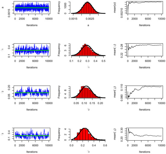
Figure 8. The Markov chain Monte Carlo (MCMC) plots for data set I using the BBXEx model.

Table 8 shows some descriptive statistics for data set I utilizing the BBXEx distribution and its marginals.

Table 8. Some descriptive statistics for data set I.

Model ↓ Measures →	Mean	Variance	Skewness	Kurtosis	Correlation
$X_1$	$39.3687$	$399.6321$	$0.14693$	$1.9697$	−
$X_2$	$31.9867$	$498.3108$	$0.5039$	$1.8693$	−
$min(X_1,X_2)$	$43.6987$	$411.3377$	$0.0278$	$1.6574$	−
$(X_1,X_2)$	−	−	$0.1986$	$1.3631$	$0.5117$

According to Table 8, it is clear that the bivariate data has positively skewed with platykurtic. Moreover, the correlation between the two random variables is positive and strong. Positive correlation is a relationship between two variables in which both variables move in tandem that is, in the same direction.

Table 9, Table 10 and Table 11 list estimation summaries for the BBXEx model and the competitive models based on Type-II censored data using data set I.

Table 9. The MLEs and goodness-of-fit measures based on Type-II censored data at $r=10$ using data set I.

		Model
Statistic		BBXEx	BGEx	BEx	BGuEx	BGLFR	BW	BEW	BGPW
$\widehat{{\gamma }_1}$	MLE	$0.5739$	$0.0004$	$0.0048$	$4.2907$	$0.9196$	$0.4709$	$1.3010$	$0.1198$
	STER	$0.1423$	$0.0003$	$0.0024$	$1.1534$	$0.5953$	$0.1674$	$1.8207$	$0.0627$
$\widehat{{\gamma }_2}$	MLE	$0.0507$	$0.5871$	$0.0069$	$0.3603$	$0.3768$	$0.3598$	$0.1336$	$0.2818$
	STER	$0.0491$	$0.5806$	$0.0068$	$0.3491$	$0.8904$	$0.2277$	$0.2562$	$0.2554$
$\widehat{{\gamma }_3}$	MLE	$0.2324$	$3.2979$	$0.0683$	$1.6571$	$0.4138$	$0.8995$	$0.5511$	$1.1938$
	STER	$0.0892$	$1.3024$	$0.0227$	$0.6405$	$0.2839$	$0.2445$	$0.8463$	$0.5997$
$\widehat{a}$	MLE	$0.0123$	$0.1405$	−	$6.9336$	$0.0026$	$0.0190$	$0.0107$	$0.2248$
	STER	$0.0025$	$0.0222$	−	$1.6581$	$0.0105$	$0.0134$	$0.0621$	$0.1044$
$\widehat{b}$	MLE	−	−	−	$2.7670$	$0.0012$	−	$1.2228$	−
	STER	−	−	−	$0.3521$	$0.0007$	−	$1.2988$	−
AIC		$183.1820$	$249.0277$	$191.4764$	$184.1763$	$191.1341$	$158.3580$	$185.3535$	$175.1364$
CAIC		$191.1820$	$257.0277$	$195.4764$	$199.1763$	$206.1341$	$166.3580$	$200.3535$	$183.1364$
BIC		$184.3923$	$250.2380$	$192.3841$	$185.6892$	$192.6470$	$159.5683$	$186.8664$	$176.3468$
HQIC		$181.8543$	$247.7000$	$190.4806$	$182.5166$	$189.4744$	$157.0302$	$183.6938$	$173.8087$

Table 10. The MLEs and goodness-of-fit measures based on Type-II censored data at $r=20$ using data set I.

		Model
Statistic		BBXEx	BGEx	BEx	BGuEx	BGLFR	BW	BEW	BGPW
$\widehat{{\gamma }_1}$	MLE	$0.4694$	$0.0021$	$0.0052$	$1.7371$	$0.9331$	$0.2630$	$0.5056$	$0.2453$
	STER	$0.1147$	$0.0014$	$0.0021$	$0.5834$	$0.2469$	$0.0871$	$0.2269$	$0.1024$
$\widehat{{\gamma }_2}$	MLE	$0.1120$	$0.6721$	$0.0092$	$4.8482$	$0.6221$	$0.3130$	$0.0044$	$0.5688$
	STER	$0.0546$	$0.3406$	$0.0045$	$3.9168$	$0.3982$	$0.1040$	$0.0071$	$0.2910$
$\widehat{{\gamma }_3}$	MLE	$0.2746$	$2.1077$	$0.0425$	$4.5543$	$0.7142$	$0.5565$	$1.4242$	$1.3662$
	STER	$0.0795$	$0.6120$	$0.0103$	$3.2232$	$0.2611$	$0.1166$	$0.3663$	$0.6433$
$\widehat{a}$	MLE	$0.0125$	$0.0717$	−	$3.0075$	$0.0323$	$0.0521$	$0.8669$	$0.1503$
	STER	$0.0016$	$0.0110$	−	$0.9186$	$0.0200$	$0.0233$	$0.3660$	$0.0633$
$\widehat{b}$	MLE	−	−	−	$0.7050$	$0.0007$	−	$0.2049$	−
	STER	−	−	−	$0.3670$	$0.0007$	−	$0.1220$	−
AIC		$338.1156$	$417.8976$	$389.5858$	$340.7217$	$361.1384$	$338.3551$	$341.4218$	$349.6559$
CAIC		$340.7823$	$420.5643$	$391.0858$	$345.0074$	$365.4242$	$341.0217$	$345.7075$	$352.3225$
BIC		$342.0985$	$421.8805$	$392.5730$	$345.7003$	$366.1171$	$342.3380$	$346.4005$	$353.6388$
HQIC		$338.8931$	$418.6751$	$390.1689$	$341.6936$	$362.1103$	$339.1326$	$342.3937$	$350.4334$

Table 11. The MLEs and goodness-of-fit measures based on Type-II censored data at $r=30$ using data set I.

		Model
Statistic		BBXEx	BGEx	BEx	BGuEx	BGLFR	BW	BEW	BGPW
$\widehat{{\gamma }_1}$	MLE	$0.4333$	$0.0287$	$0.0101$	$3.0075$	$0.5281$	$0.3658$	$0.8348$	$0.6274$
	STER	$0.1024$	$0.0084$	$0.0027$	$0.9186$	$0.1329$	$0.0713$	$0.7409$	$0.1622$
$\widehat{{\gamma }_2}$	MLE	$0.0959$	$0.3171$	$0.0080$	$0.7050$	$0.4257$	$0.2264$	$0.1738$	$0.5415$
	STER	$0.0455$	$0.1575$	$0.0039$	$0.3670$	$0.2939$	$0.0783$	$0.1647$	$0.2412$
$\widehat{{\gamma }_3}$	MLE	$0.2842$	$1.1211$	$0.0393$	$1.7371$	$0.8251$	$0.4461$	$0.5305$	$1.3712$
	STER	$0.0676$	$0.2849$	$0.0081$	$0.5834$	$0.3469$	$0.0865$	$0.4661$	$0.5034$
$\widehat{a}$	MLE	$0.0125$	$0.0385$	−	$4.8482$	$0.0205$	$0.0757$	$0.0033$	$0.1345$
	STER	$0.0011$	$0.0069$	−	$3.9168$	$0.0192$	$0.0258$	$0.0130$	$0.0408$
$\widehat{b}$	MLE	−	−	−	$4.5543$	$0.0012$	−	$1.5365$	−
	STER	−	−	−	$3.2232$	$0.0006$	−	$0.8817$	−
AIC		$490.7070$	$609.9449$	$556.3474$	$492.9298$	$522.8255$	$539.1251$	$492.0913$	$548.0223$
CAIC		$492.3070$	$611.5449$	$557.2705$	$495.4298$	$525.3255$	$540.7251$	$494.5913$	$549.6223$
BIC		$496.3118$	$615.5496$	$560.5510$	$499.9358$	$529.8315$	$544.7299$	$499.0973$	$553.6271$
HQIC		$492.5001$	$611.7379$	$557.6922$	$495.1710$	$525.0668$	$540.9182$	$494.3326$	$549.8153$

Regarding Table 9, Table 10 and Table 11, it is clear that both BW and BGPW models are better than the BBXEx model in case of small values of r as seen in Table 9, whereas the BBXEx model provides better fit than other competitive models when the value of r grows as seen in Table 10 and Table 11.

7.2. Data Set II: Motor Data

This data is reported in [62], and it represents the failure times of a parallel system constituted by two identical motors in days. We consider the BBXEx model to analyze the censored samples. We fit at first the marginals $X_1$, $X_2$ and $max(X_1,X_2)$ separately on the motor data. The MLEs of the parameters ($\gamma ,a$) of the BXEx model for $X_1$, $X_2$ and $min(X_1,X_2)$ are ($1.548,0.004$), ($1.233,0.003$) and ($1.343,0.004$), respectively with STER ($0.465,0.0003$), ($0.359,0.0003$) and ($0.394,0.0003$). The $-L$, KS distance and its p-value for the marginals are reported in Table 12.

Table 12. The L, KS and p-values for the marginals using data set II.

	${\mathit{X}}_1$			${\mathit{X}}_2$			$min({\mathit{X}}_1,{\mathit{X}}_2)$
Model	$-\mathit{L}$	KS	p-Value	$-\mathit{L}$	KS	p-Value	$-\mathit{L}$	KS	p-Value
BXEx	$99.494$	$0.222$	$0.338$	$102.935$	$0.114$	$0.953$	$99.026$	$0.180$	$0.604$

It is clear that the BXEx model fits the data for the marginals. The fitted PDF, estimated CDF, PP, scatter and TTT plots are displayed in Figure 9, Figure 10, Figure 11 and Figure 12.

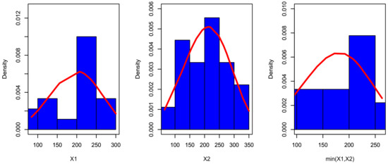
Figure 9. The fitted PDF for $X_1$, $X_2$ and $min(X_1,X_2)$ for data set II.

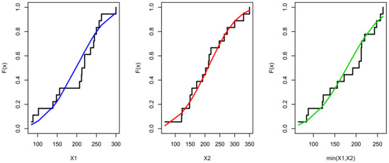
Figure 10. The estimated CDF for $X_1$, $X_2$ and $min(X_1,X_2)$ for data set II.

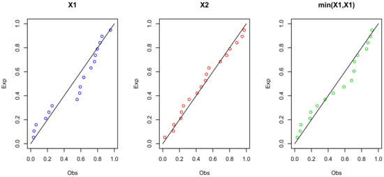
Figure 11. The PP plots for $X_1$, $X_2$ and $min(X_1,X_2)$ for data set II.

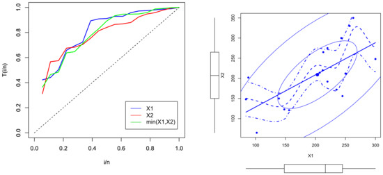
Figure 12. The TTT (left panel) and scatter (right panel) plots for data set II.

From Figure 12, it is clear that the marginals have increasing HRF. Now, we fit the BBXEx model based on a complete sample. In the enclosed Table 13, we provide the MLEs with its corresponding STER, $-L$, AIC, CAIC, BIC and HQIC values for tested distributions.

Table 13. The MLE and goodness-of-fit measures based on data set II.

		Model
Statistic		BBXEx	BGEx	BW	BGPW	BEx	BGuEx	BEW	BGLFR
$\widehat{{\gamma }_1}$	MLE	$0.362$	$2.454$	$0.200$	$1.559$	$0.002$	$3.066$	$30.138$	$0.417$
	STER	$0.129$	$1.019$	$0.051$	$3.043$	$0.0005$	$1.209$	$9.676$	$9.71\times {10}^{-7}$
$\widehat{{\gamma }_2}$	MLE	$0.424$	$2.880$	$0.238$	$1.858$	$0.002$	$4.485$	$24.135$	$0.486$
	STER	$0.137$	$1.116$	$0.052$	$3.679$	$0.0005$	$1.747$	$7.676$	$1.05\times {10}^{-6}$
$\widehat{{\gamma }_3}$	MLE	$0.907$	$6.064$	$0.339$	$3.719$	$0.005$	$8.043$	$61.805$	$1.019$
	STER	$0.198$	$1.811$	$0.062$	$7.263$	$0.0009$	$2.229$	$6.378$	$1.33\times {10}^{-6}$
$\widehat{a}$	MLE	$0.003$	$0.014$	$0.039$	$0.029$	−	$6.311$	$0.520$	$6.99\times {10}^{-5}$
	STER	$0.0002$	$0.002$	$0.016$	$0.056$	−	$0.851$	$0.051$	$1.09\times {10}^{-5}$
$\widehat{b}$	MLE	−	−	−	−	−	$10.533$	$0.325$	$0.001$
	STER	−	−	−	−	−	$0.863$	$0.084$	$0.0008$
AIC		$667.52$	$678.46$	$853.90$	$871.58$	$717.46$	$679.26$	$688.54$	$673.54$
CAIC		$670.59$	$681.53$	$856.98$	$874.66$	$719.17$	$684.26$	$693.54$	$678.54$
BIC		$671.08$	$682.02$	$857.47$	$875.14$	$720.13$	$683.71$	$692.99$	$677.99$
HQIC		$668.01$	$678.95$	$854.39$	$872.07$	$717.83$	$679.87$	$689.15$	$674.15$

From Table 13, it is clear that, the BBXEx model provides a better fit than the other competitive models. The BCI for the BBXEx parameters are $[0.287,0.438]$, $[0.299,0.543]$, $[0.811,1.236]$ and $[0.002,0.005]$, respectively. The BSEs with its STER for the BBXEx model using data set II are listed in Table 14.

Table 14. The BSEs for the BBXEx distribution using data set II.

Statistic ↓ Parameter →	a	${\gamma }_1$	${\gamma }_2$	${\gamma }_3$
Estimation	$0.0033$	$0.3674$	$0.4191$	$0.8892$
STER	$0.0001$	$0.0856$	$0.0906$	$0.1346$
Credible Interval	$[0.0031,0.0062]$	$[0.1996,0.4768]$	$[0.2416,0.5642]$	$[0.6255,1.3605]$

The results presented in Table 14 are very similar to the MLE results. For the BSE of the BBXEx parameters, the estimated hyper-parameters are $a_1=354.948$,$a_2=7.899$, $a_3=$$9.601$ and $a_4=$$21.055$ whereas $b_1=106405.318$,$b_2=21.849$, $b_3=$$22.623$ and $b_4=$$23.216$. The MCMC plots for data set II based on complete sample are displayed in Figure 13.

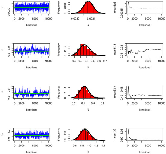
Figure 13. The MCMC plots for data set II using the BBXEx model based on the complete sample.

Here, we fit the BBXEx model on data set II based on censored samples. In the enclosed Table 15, Table 16 and Table 17, we provide the MLEs, BSEs, AIC, CAIC, BIC and HQIC values for all tested models.

Table 15. The MLEs and goodness-of-fit measures based on the censored sample at $r=7$.

		Model
Statistic		BBXEx	BGEx	BW	BGPW	BEx	BGuEx	BEW	BGLFR
$\widehat{{\gamma }_1}$	MLE	$0.287$	$0.001$	$0.197$	$0.129$	$0.003$	$1.715$	$27.831$	$0.455$
	STER	$0.160$	$0.0009$	$0.085$	$0.070$	$0.001$	$1.094$	$15.865$	$1.4\times {10}^{-5}$
$\widehat{{\gamma }_2}$	MLE	$0.220$	$1.788$	$0.454$	$0.439$	$0.001$	$1.231$	$20.518$	$0.317$
	STER	$0.114$	$0.918$	$0.097$	$0.175$	$0.0006$	$0.738$	$10.467$	$1.7\times {10}^{-5}$
$\widehat{{\gamma }_3}$	MLE	$0.754$	$0.003$	$0.331$	$0.268$	$0.003$	$3.998$	$69.221$	$1.138$
	STER	$0.233$	$0.001$	$0.101$	$0.096$	$0.0009$	$1.708$	$7.468$	$1.5\times {10}^{-5}$
$\widehat{a}$	MLE	$0.003$	$0.012$	$0.018$	$0.223$	−	$1.629$	$0.393$	$6.1\times {10}^{-5}$
	STER	$0.0004$	$0.003$	$0.013$	$0.069$	−	$0.764$	$0.067$	$2.4\times {10}^{-5}$
$\widehat{b}$	MLE	−	−	−	−	−	$50.678$	$0.644$	$1.9\times {10}^{-5}$
	STER	−	−	−	−	−	$27.828$	$0.210$	$0.002$
AIC		$284.01$	$530.81$	$327.82$	$354.68$	$293.69$	$284.21$	$283.65$	$285.16$
CAIC		$304.01$	$550.81$	$347.82$	$374.68$	$301.69$	$344.21$	$343.65$	$345.16$
BIC		$283.79$	$530.59$	$327.60$	$354.46$	$293.53$	$283.94$	$283.38$	$284.89$
HQIC		$281.34$	$528.13$	$325.15$	$352.01$	$291.69$	$280.87$	$280.31$	$281.82$

Table 16. The MLE and goodness-of-fit measures based on the censored sample at $r=10$.

		Model
Statistic		BBXEx	BGEx	BW	BGPW	BEx	BGuEx	BEW	BGLFR
$\widehat{{\gamma }_1}$	MLE	$0.318$	$0.003$	$0.184$	$0.169$	$0.002$	$2.402$	$27.989$	$0.438$
	STER	$0.156$	$0.002$	$0.068$	$0.078$	$0.0009$	$1.275$	$13.848$	$3\times {10}^{-6}$
$\widehat{{\gamma }_2}$	MLE	$0.324$	$1.053$	$0.362$	$0.424$	$0.001$	$2.437$	$26.847$	$0.415$
	STER	$0.137$	$0.454$	$0.076$	$0.154$	$0.0006$	$1.134$	$10.998$	$3\times {10}^{-6}$
$\widehat{{\gamma }_3}$	MLE	$0.882$	$0.008$	$0.334$	$0.363$	$0.004$	$6.554$	$72.792$	$1.112$
	STER	$0.238$	$0.0028$	$0.083$	$0.111$	$0.0009$	$2.150$	$7.181$	$4\times {10}^{-6}$
$\widehat{a}$	MLE	$0.004$	$0.0078$	$0.026$	$0.201$	−	$6.886$	$0.438$	$7.1\times {10}^{-5}$
	STER	$0.0003$	$0.002$	$0.015$	$0.056$	−	$16.361$	$0.059$	$1.8\times {10}^{-5}$
$\widehat{b}$	MLE	−	−	−	−	−	$10.185$	$0.520$	$8.3\times {10}^{-4}$
	STER	−	−	−	−	−	$24.175$	$0.154$	$0.001$
AIC		$386.63$	$677.15$	$471.29$	$499.95$	$410.95$	$391.44$	$393.62$	$389.69$
CAIC		$394.63$	$685.15$	$479.29$	$507.95$	$414.95$	$406.44$	$408.62$	$404.69$
BIC		$387.84$	$678.36$	$472.51$	$501.16$	$411.86$	$392.95$	$395.13$	$391.21$
HQIC		$385.29$	$675.82$	$469.97$	$498.62$	$409.95$	$389.78$	$391.96$	$388.04$

Table 17. The MLE and goodness-of-fit measures based on the censored sample at $r=15$.

		Model
Statistic		BBXEx	BGEx	BW	BGPW	BEx	BGuEx	BEW	BGLFR
$\widehat{{\gamma }_1}$	MLE	$0.396$	$0.012$	$0.208$	$0.311$	$0.002$	$3.244$	$24.801$	$0.431$
	STER	$0.149$	$0.004$	$0.056$	$0.110$	$0.0007$	$1.374$	$9.259$	$1.3\times {10}^{-6}$
$\widehat{{\gamma }_2}$	MLE	$0.395$	$0.619$	$0.271$	$0.443$	$0.002$	$3.271$	$25.415$	$0.394$
	STER	$0.143$	$0.232$	$0.059$	$0.157$	$0.0006$	$1.333$	$8.847$	$1.7\times {10}^{-6}$
$\widehat{{\gamma }_3}$	MLE	$0.942$	$0.027$	$0.335$	$0.577$	$0.005$	$7.709$	$60.435$	$1.059$
	STER	$0.221$	$0.006$	$0.068$	$0.172$	$0.0009$	$2.264$	$5.453$	$2.7\times {10}^{-6}$
$\widehat{a}$	MLE	$0.004$	$0.004$	$0.034$	$0.151$	−	$6.322$	$0.521$	$7.7\times {10}^{-5}$
	STER	$0.0002$	$0.001$	$0.016$	$0.041$	−	$3.099$	$0.054$	$1.3\times {10}^{-5}$
$\widehat{b}$	MLE	−	−	−	−	−	$10.358$	$0.3264$	$0.002$
	STER	−	−	−	−	−	$4.942$	$0.088$	$8.9\times {10}^{-4}$
AIC		$557.96$	$860.01$	$708.24$	$736.17$	$600.83$	$567.33$	$573.49$	$563.39$
CAIC		$561.96$	$864.01$	$712.24$	$740.17$	$603.01$	$573.99$	$580.16$	$570.05$
BIC		$560.79$	$862.85$	$711.08$	$738.99$	$602.96$	$570.87$	$577.03$	$566.93$
HQIC		$557.93$	$859.99$	$708.21$	$736.14$	$600.81$	$567.29$	$573.45$	$563.35$

From Table 15, Table 16 and Table 17 it is observed that, the BBXEx model provides a better fit than the other competitive models. Table 18 shows some descriptive statistics for data set II utilizing the BBXEx distribution and its marginals.

Table 18. Some descriptive statistics for data set II.

Model ↓ Measures →	Mean	Variance	Skewness	Kurtosis	Correlation
$X_1$	$165.3615$	$4011.2368$	$-0.5253$	$2.0475$	−
$X_2$	$205.9992$	$5793.1260$	$0.1610$	$2.2299$	−
$min(X_1,X_2)$	$229.0103$	$4669.9687$	$-0.0332$	$2.0445$	−
$(X_1,X_2)$	−	−	$0.2394$	$1.0097$	$0.7531$

According to Table 18, it is clear that the bivariate data has positively skewed with platykurtic. Moreover, the correlation between the two random variables is positive and strong. Positive correlation is a relationship between two variables in which both variables move in tandem that is, in the same direction.

8. Conclusions

In this paper, we have proposed a bivariate BBX-G family of distributions, whose marginal distributions are BX-G families. It was found that the BBX-G family is suitable of modeling positive skewness and symmetric data sets with leptokurtic phenomena. Moreover, the stress–strength reliability does not depend on the baseline function, but only on the family parameters. The family parameters have been estimated using Bayesian and maximum likelihood methods based on complete and Type-II censored samples, and it was found that the two methods performed quite well in estimating the family parameters. The usefulness of the proposed family is illustrated by two real data sets and it was found that the new family provides a better fit than others sub models and non-nested models. Finally, we can say that the new family will serve as an alternative model to other models available in the literature for modeling positive real data in many areas.

References

- Burr, I.W. Cumulative frequency functions. Ann. Math. Stat. 1942, 18, 215–232. [Google Scholar] [CrossRef]
- Sartawi, H.A.; Abu-Salih, M.S. Bayesian prediction bounds for the Burr Type X model. Commun. Stat. Theory Methods 1991, 20, 2307–2330. [Google Scholar] [CrossRef]
- Jaheen, Z.F. Empirical bayes estimation of the reliability and failure rate functions of the Burr Type X failure model. J. Appl. Stat. Sci. 1996, 3, 281–288. [Google Scholar]
- Ahmad, K.E.; Fakhry, M.E.; Jaheen, Z.F. Empirical Bayes estimation of p(Y<X) and characterizations of Burr Type X model. J. Stat. Plan. Inference 1997, 64, 297–308. [Google Scholar]
- Surles, J.G.; Padgett, W.J. Inference for p(Y<X) in the Burr Type X model. Commun. Stat. Theory Methods 1998, 7, 225–238. [Google Scholar]
- Raqab, M.Z. Order statistics from the Burr Type X model. Comput. Math. Appl. 1998, 36, 111–120. [Google Scholar] [CrossRef]
- Mousa, M.A. Inference and prediction for the Burr Type X model based on records. Stat. A J. Theor. Appl. Stat. 2001, 35, 415–425. [Google Scholar]
- Khaleel, M.A.; Ibrahim, N.A.; Shitan, M.; Merovci, F.; Rehman, E. New extension of Burr Type X distribution properties with application. J. King Saud Univ. Sci. 2017, 30, 450–457. [Google Scholar] [CrossRef]
- Yousof, H.M.; Afify, A.Z.; Hamedani, G.G.; Gokarna, A. The Burr X generator of distributions for lifetime data. J. Stat. Theoryand Appl. 2017, 16, 288–305. [Google Scholar] [CrossRef]
- Alzaatreh, A.; Lee, C.; Famoye, F. A new method for generating families of continuous distributions. Metron 2013, 71, 63–79. [Google Scholar] [CrossRef]
- Alizadeh, M.; Cordeiro, G.M.; Nascimento, A.D.; Lima, M.D.; Ortega, E.M. Odd Burr generalized family of distributions with some applications. J. Stat. Comput. Simul. 2016, 83, 326–339. [Google Scholar] [CrossRef]
- Tahir, M.H.; Zubair, M.; Mansoor, M.; Cordeiro, G.M.; Alizadeh, M.; Hamedani, G.G. A new Weibull-G family of distributions. Hacet. J. Math. Stat. 2016, 45, 629–647. [Google Scholar]
- Cordeiro, G.M.; Alizadeh, M.; Ozel, G.; Hosseini, B.; Ortega, E.M.; Altun, E. The generalized odd log-logistic family of distributions: Properties, regression models and applications. J. Stat. Simul. 2017, 87, 908–932. [Google Scholar] [CrossRef]
- Silva, F.G.; Percontini, A.; Brito, E.; Ramos, M.W.; Venancio, R.; Cordeiro, G.M. The odd Lindley-G family of distributions. Austrian J. Stat. 2017, 46, 65–87. [Google Scholar] [CrossRef]
- El-Morshedy, M.; Eliwa, M.S. The odd flexible Weibull-H family of distributions: Properties and estimation with applications to complete and upper record data. Filomat 2019. [Google Scholar] [CrossRef]
- Alizadeh, M.; Afify, A.Z.; Eliwa, M.S.; Ali, S. The odd log-logistic Lindley-G family of distributions: Properties, Bayesian and non-Bayesian estimation with applications. Comput. Stat. 2019. [Google Scholar] [CrossRef]
- Eliwa, M.S.; El-Morshedy, M.; Afify, A.Z. The odd Chen generator of distributions: Properties and estimation methods with applications in medicine and engineering. J. Natl. Sci. Found. Sri Lanka 2020, 48, 1–23. [Google Scholar]
- Balakrishnan, N.; Lai, C.D. Continuous Bivariate Distributions, 2nd ed.; Wiley: New York, NY, USA, 2009. [Google Scholar]
- Chalikias, M.S. The selection of high school teachers in Greek public schools: An application of generalized linear models. Appl. Math. Sci. 2012, 6, 3025–3035. [Google Scholar]
- Dimitrakopoulou, T.; Adamidis, K.; Loukas, S. Bivariate extended exponential-geometric distributions. Commun. Stat. Theory Methods 2012, 41, 1129–1150. [Google Scholar] [CrossRef]
- Adamidis, K.; Dimitrakopoulou, T.; Loukas, S. On an extension of the exponential geomeric distribution. Stat. Probab. Lett. 2005, 73, 259–269. [Google Scholar] [CrossRef]
- Bidram, H. A bivariate compound class of geometric-Poisson and lifetime distributions. J. Stat. Appl. Probab. 2013, 2, 21–25. [Google Scholar] [CrossRef]
- Kundu, D.; Gupta, A.K. On bivariate Weibull-geometric distribution. J. Multivar. Anal. 2014, 123, 19–29. [Google Scholar] [CrossRef]
- El-Bassiouny, A.H.; EL-Damcese, M.A.; Mustafa, A.; Eliwa, M.S. Bivariate exponentaited generalized Weibull-Gompertz distribution. J. Appl. Probab. Stat. 2016, 11, 25–46. [Google Scholar]
- El-Gohary, A.; El-Bassiouny, A.H.; El-Morshedy, M. Bivariate exponentiated modified Weibull extension distribution. J. Stat. Probab. 2016, 5, 67–78. [Google Scholar] [CrossRef]
- Roozegar, R.; Jafari, A.A. On bivariate generalized linear failure rate-power series class of distribution. Iran. J. Sci. Technol. Trans. A 2017, 41, 693–706. [Google Scholar] [CrossRef]
- Kundu, D.; Gupta, R.D. A class of bivariate models with proportional reversed hazard marginals. Sankhya 2010, 72, 236–253. [Google Scholar] [CrossRef]
- Sarabia, J.M.; Prieto, F.; Jorda, V. Bivariate beta-generated distributions with applications to well-being data. J. Stat. Distrib. Appl. 2014. [Google Scholar] [CrossRef]
- Balakrishnan, N.; Ristic, M.M. Multivariate families of gamma-generated distributions with finite or infinite support or below the diagonal. J. Multivar. Anal. 2016, 143, 194–207. [Google Scholar] [CrossRef]
- Roozegar, R.; Jafari, A.A. On bivariate exponentiated extended Weibull family of distributions. Cienc. Nautr 2016, 38, 564–576. [Google Scholar] [CrossRef]
- Ghosh, I.; Hamedani, G.G. On the Ristic-Balakrishnan distribution: Bivariate extension and characterizations. J. Stat. Theory Prac. 2017. [Google Scholar] [CrossRef]
- Eliwa, M.S.; El-Morshedy, M. Bivariate Gumbel-G family of distributions: Statistical properties, Bayesian and non-Bayesian estimation with application. Ann. Data Sci. 2019, 6, 39–60. [Google Scholar] [CrossRef]
- Eliwa, M.S.; El-Morshedy, M. Bivariate odd Weibull-G family of distributions: Properties, Bayesian and non-Bayesian estimation with bootstrap confidence intervals and application. J. Taibah Univ. Sci. 2020, 14, 1–22. [Google Scholar]
- Eliwa, M.S.; Alhussain, Z.A.; Ahmed, E.A.; Salah, M.M.; Ahmed, H.H.; El-Morshedy, M. Bivariate Gompertz generator of distributions: Statistical properties and estimation with application to model football data. J. Natl. Sci. Found. Sri Lanka 2020, 48, 54–72. [Google Scholar]
- Marshall, A.W.; Olkin, I. A multivariate exponential model. J. Am. Stat. Assoc. 1967, 62, 30–44. [Google Scholar] [CrossRef]
- Gupta, R.C.; Gupta, P.L.; Gupta, R.D. Modeling failure time data by Lehmann alternatives. Commun. Stat. Theory Andm. 1998, 27, 887–904. [Google Scholar] [CrossRef]
- Nelsen, R.B. An Introduction to Copulas, 2nd ed.; Springer: New York, NY, USA, 1999. [Google Scholar]
- Lehmann, E.L. Some concepts of dependence. Ann. Math. 1966, 37, 1137–1153. [Google Scholar] [CrossRef]
- Barlow, R.E.; Proschan, F. Statistical Theory of Reliability and Life Testing; Probability Models: Silver Spring, MD, USA, 1981. [Google Scholar]
- Domma, F. Some properties of the bivariate Burr Type III distribution. Statistics 2010, 44, 203–215. [Google Scholar] [CrossRef]
- Nadarajah, S.; Kotz, S. The exponentiated Type distributions. Acta Appl. Math. 2006, 92, 97–111. [Google Scholar] [CrossRef]
- Arcagnia, A.; Porrob, F. The graphical representation of inequality. Rev. Colomb. De Estad. 2014, 37, 419–436. [Google Scholar] [CrossRef]
- Mardia, K.V. Measures of multivariate skewness and kurtosis with applications. Biometrika 1970, 57, 519–530. [Google Scholar] [CrossRef]
- Basu, A.P. Bivariate failure rate. Am. Stat. 1971, 66, 103–104. [Google Scholar] [CrossRef]
- Bismi, G. Bivariate Burr Distributions. Ph.D Thesis, Cochin University of Science and Technology, Kochi, India, 2005. [Google Scholar]
- Holland, P.W.; Wang, Y.J. Dependence function for continuous bivariate densities. Commun. Stat. Theory Methods 1987, 16, 863–876. [Google Scholar] [CrossRef]
- Balakrishnan, N.; Kim, J.A. EM Algorithm for Type-II Right Censored Bivariate Normal Data in Parametric and Semiparametric Models with Applications to Reliability, Survival Analysis, and Quality of Life; Birkhuser: Boston, MA, USA, 2004; pp. 177–210. [Google Scholar]
- Metropolis, N.; Rosenbluth, A.W.; Rosenbluth, M.N.; Teller, A.H.; Teller, E. Equation of state calculations by fast computing machines. J. Chem. Phys. 1953, 21, 1087–1091. [Google Scholar] [CrossRef]
- Hastings, W.K. Monte Carlo sampling methods using Markov chains and their applications. Biometrika 1970, 57, 97–109. [Google Scholar] [CrossRef]
- Robert, C.P.; Casella, G. Monte Carlo Statistical Methods; Springer: New York, NY, USA, 2004. [Google Scholar]
- Casella, G. Monte Carlo Statistical Methods. Ph.D. Thesis, University of Florida, Gainesville, FL, USA, 2004. [Google Scholar]
- El-Sherpieny, E.S.; Muhammed, H.Z.; Almetwally, E.M. Parameter estimation of the bivariate Weibull distribution under progressive Type-II censored samples. J. Mod. Appl. Stat. Methods 2020, 19, 230–251. [Google Scholar]
- Kolmogorov, A.; Smirnov, N. Confidence limits for an unknown distribution function. Ann. Math. Stat. 1941, 4, 461–463. [Google Scholar] [CrossRef]
- Hurvich, C.M.; Tsai, C.L. A corrected Akaike information criterion for vector autoregressive model selection. J. Time Ser. 1993, 14, 271–279. [Google Scholar] [CrossRef]
- Zhao, X.M. Bayesian information criterion (BIC). Encyclopedia Syst. Biol. 2013, 73, 35–47. [Google Scholar]
- Hannan, E.J.; Quinn, B.G. The determination of the order of an auto regression. J. R. Stat. Soc. 1979, 41, 190–195. [Google Scholar]
- Meintanis, S.G. Test of fit for Marshall–Olkin distributions with applications. J. Stat. Plan. Inference 2007, 137, 3954–3963. [Google Scholar] [CrossRef]
- Ibrahim, M.; Eliwa, M.S.; El-Morshedy, M. Bivariate exponentiated generalized linear exponential distribution: Properties, inference and applications. J. Appl. Probab. Stat. 2019, 14, 1–23. [Google Scholar]
- El-Morshedy, M.; Eliwa, M.S.; El-Gohary, A.; Khalil, A.A. Bivariate exponentiated discrete Weibull distribution: Statistical properties, estimation, simulation and applications. Math. Sci. 2019. [Google Scholar] [CrossRef]
- Kruschke, J. Doing Bayesian Data Analysis: A Tutorial with R, Jags and Stan; Academic Press: Cambridge, MA, USA, 2014. [Google Scholar]
- Makowski, D.; Ben-Shachar, M.S.; Lüdecke, D. Bayes test R: Describing effects and their uncertainty, existence and significance within the Bayesian framework. J. Open Source Softw. 2019, 4, 15–41. [Google Scholar] [CrossRef]
- Relia staff. Using QALT models to analyze system configurations with load sharing. Reliab. Edge 2002, 3, 1–4. [Google Scholar]
© 2020 by the authors. Licensee MDPI, Basel, Switzerland. This article is an open access article distributed under the terms and conditions of the Creative Commons Attribution (CC BY) license (http://creativecommons.org/licenses/by/4.0/).