Figure 1.
The surface plots of the joint probability density function (PDF) for and and , respectively.
Figure 1.
The surface plots of the joint probability density function (PDF) for and and , respectively.
Figure 2.
The surface plots of the joint reliability function (RF) for and and , respectively.
Figure 2.
The surface plots of the joint reliability function (RF) for and and , respectively.
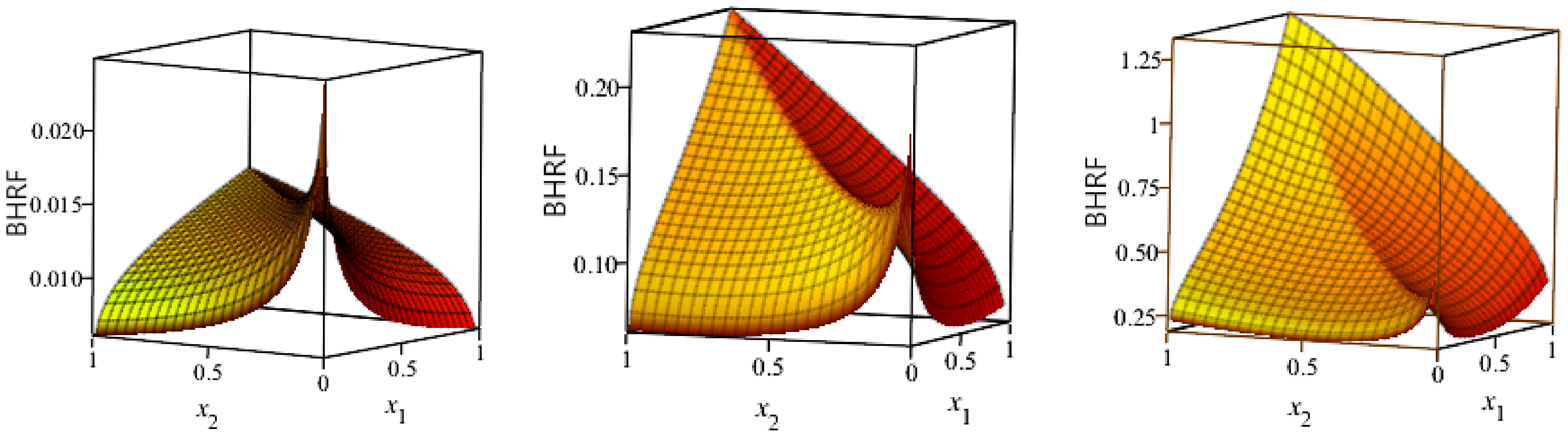
Figure 3.
The surface plots of the bivariate hazard rate function (BHRF) for and and , respectively.
Figure 3.
The surface plots of the bivariate hazard rate function (BHRF) for and and , respectively.
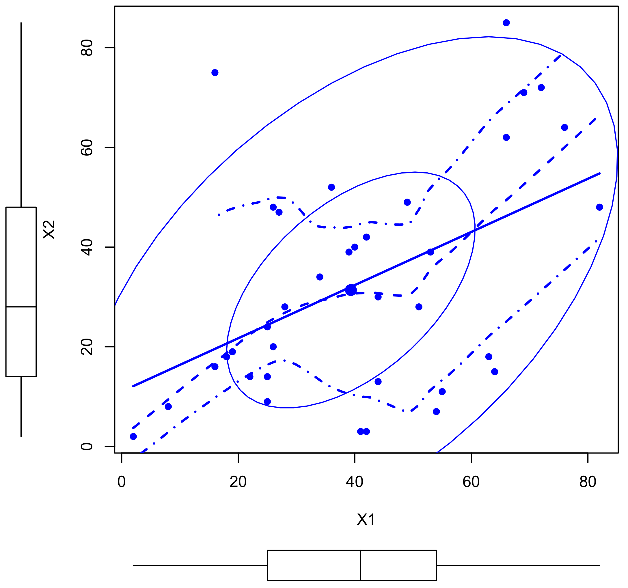
Figure 4.
The scatter plot for data set I.
Figure 4.
The scatter plot for data set I.
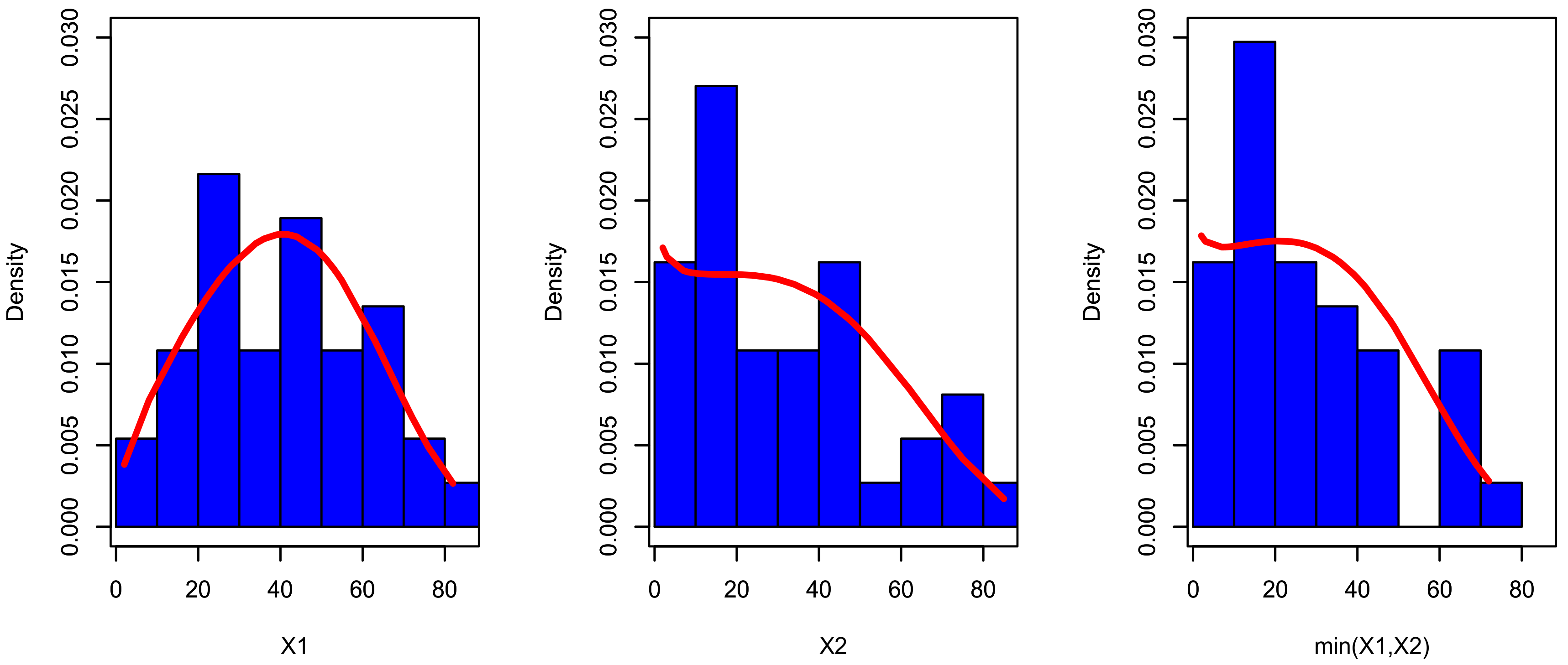
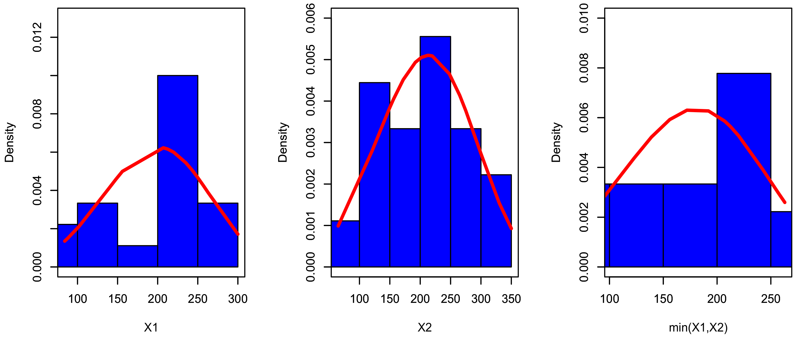
Figure 5.
The fitted PDF for , and for data set I.
Figure 5.
The fitted PDF for , and for data set I.
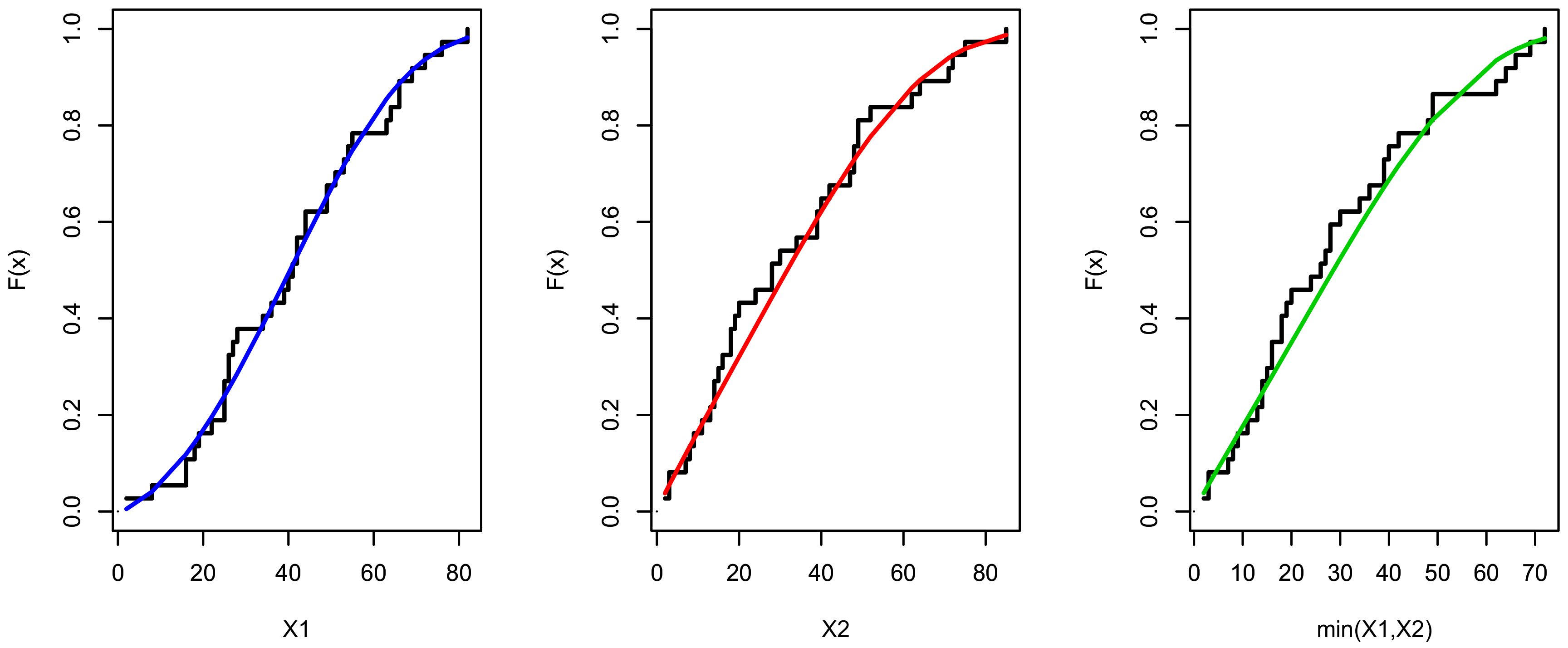
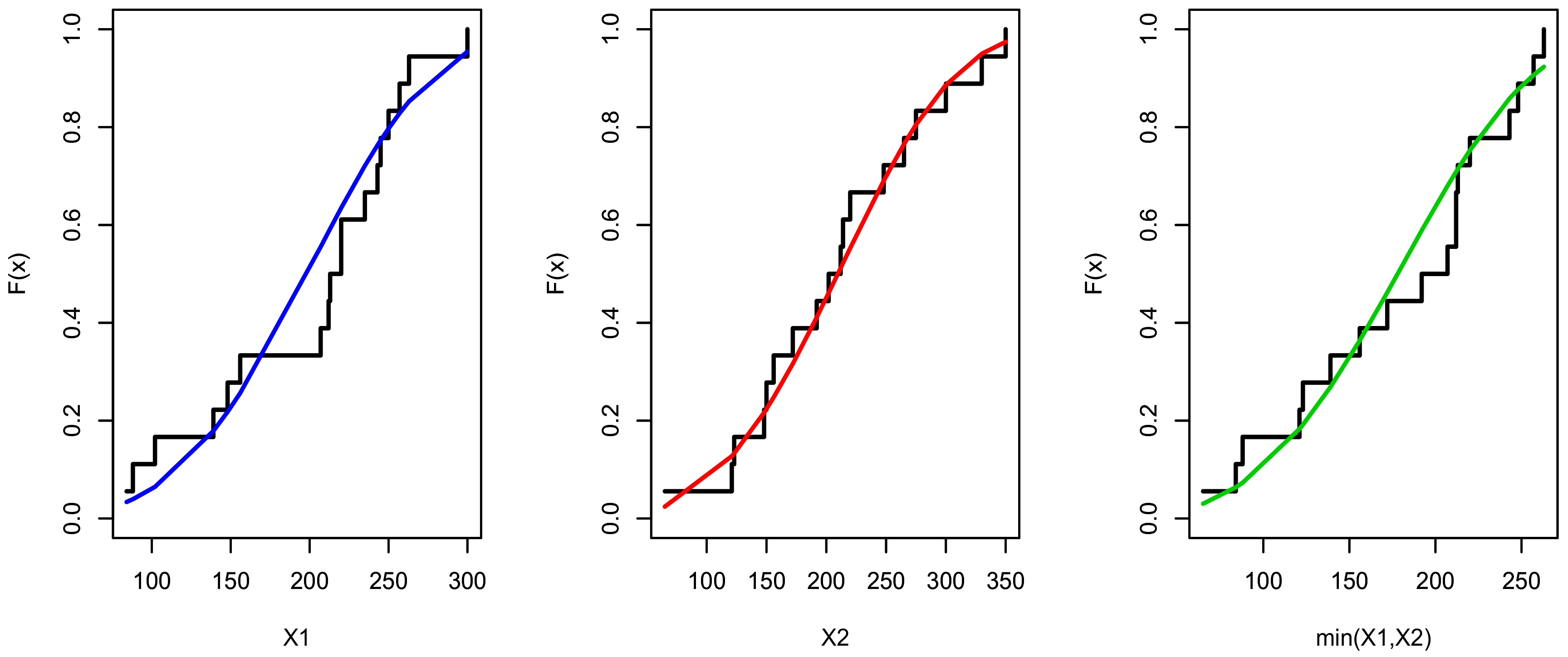
Figure 6.
The estimated cumulative distribution function (CDF) for , and for data set I.
Figure 6.
The estimated cumulative distribution function (CDF) for , and for data set I.
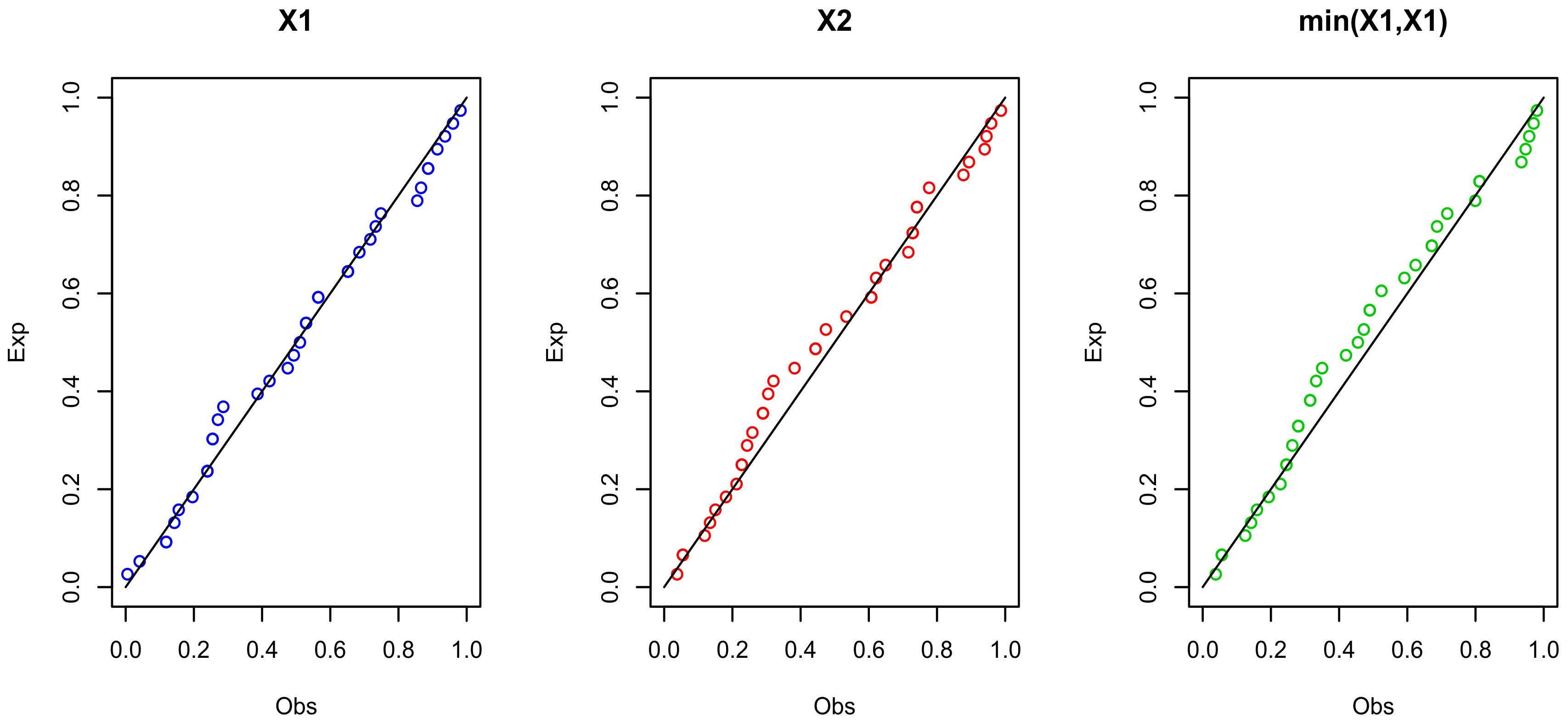
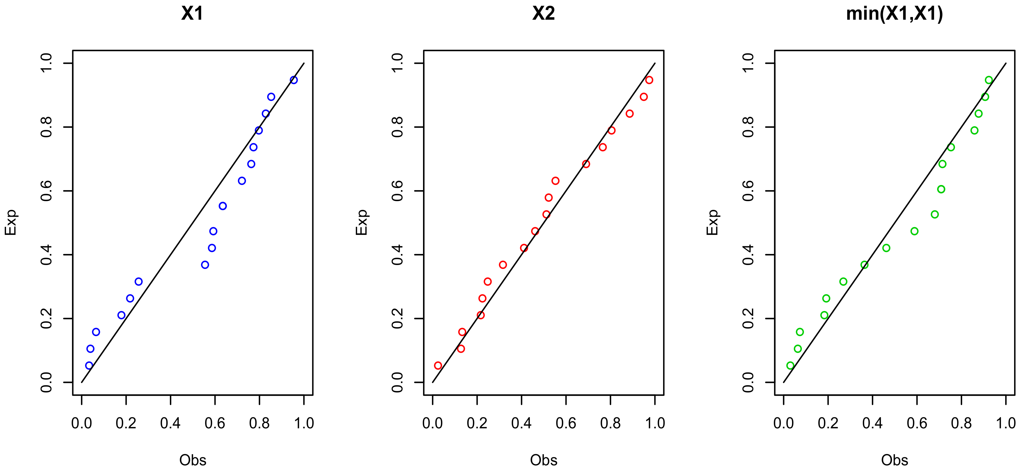
Figure 7.
The probability–probability (PP) plots for , and for data set I.
Figure 7.
The probability–probability (PP) plots for , and for data set I.
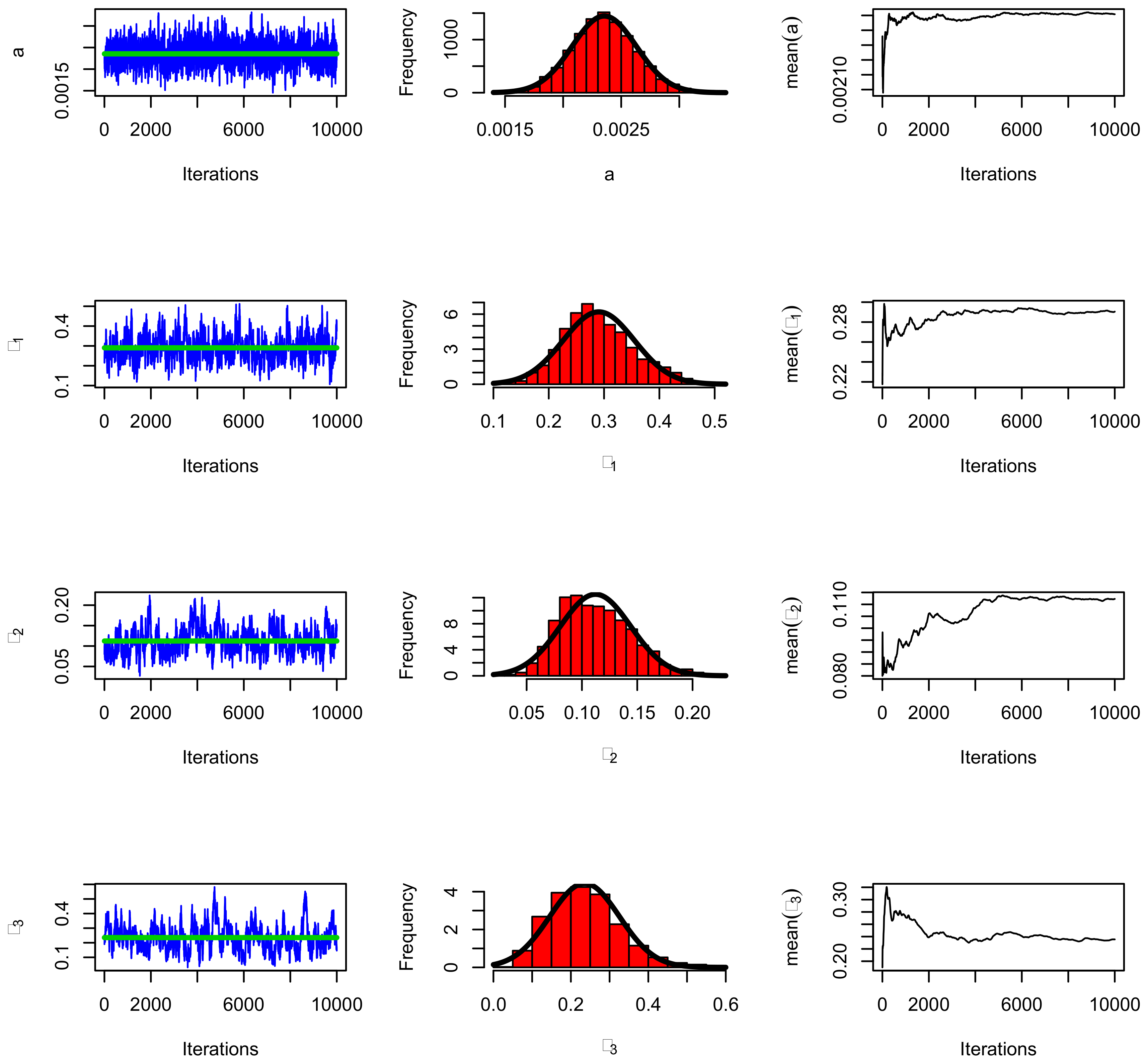
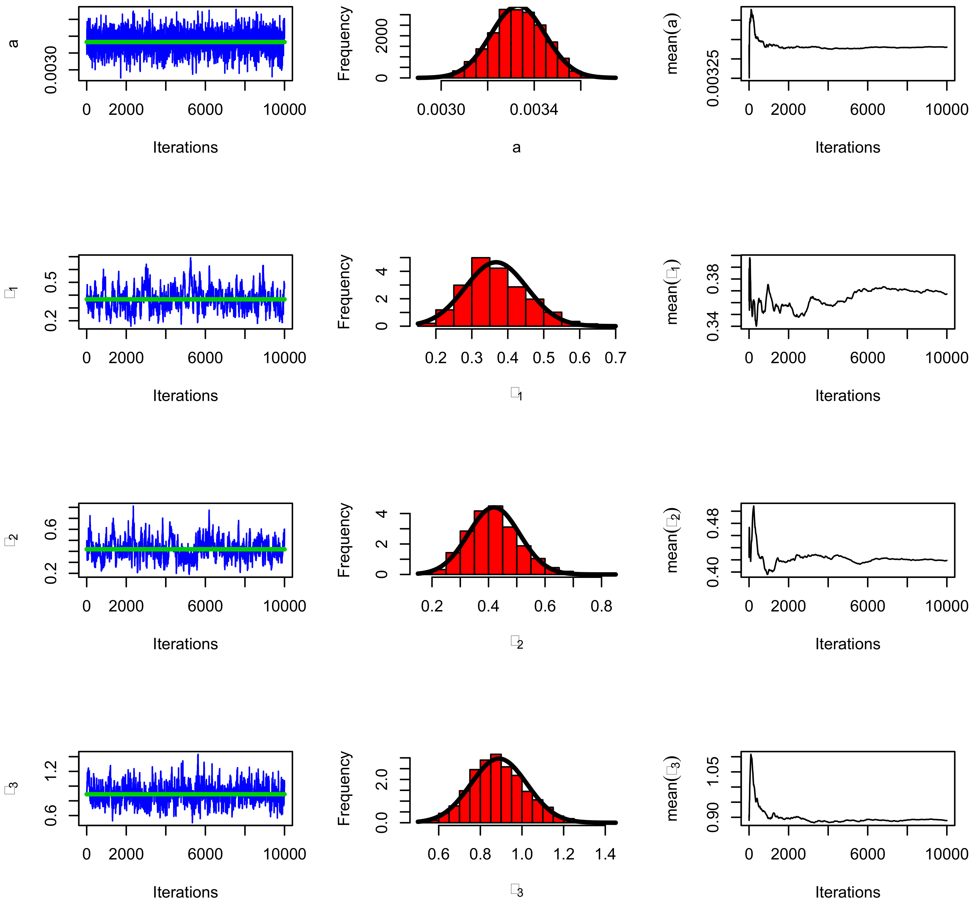
Figure 8.
The Markov chain Monte Carlo (MCMC) plots for data set I using the BBXEx model.
Figure 8.
The Markov chain Monte Carlo (MCMC) plots for data set I using the BBXEx model.
Figure 9.
The fitted PDF for , and for data set II.
Figure 9.
The fitted PDF for , and for data set II.
Figure 10.
The estimated CDF for , and for data set II.
Figure 10.
The estimated CDF for , and for data set II.
Figure 11.
The PP plots for , and for data set II.
Figure 11.
The PP plots for , and for data set II.
Figure 12.
The TTT (left panel) and scatter (right panel) plots for data set II.
Figure 12.
The TTT (left panel) and scatter (right panel) plots for data set II.
Figure 13.
The MCMC plots for data set II using the BBXEx model based on the complete sample.
Figure 13.
The MCMC plots for data set II using the BBXEx model based on the complete sample.
Table 1.
The correlation, skewness and kurtosis measures of the Burr X-exponential (BBXEx) (1.5,0.6,,1.5) distribution.
Table 1.
The correlation, skewness and kurtosis measures of the Burr X-exponential (BBXEx) (1.5,0.6,,1.5) distribution.
| Measures | | | | | | | | | | |
| Correlation | | | | | | | | | | |
| Skewness | | | | | | | | | | |
| Kurtosis | | | | | | | | | | |
Table 2.
Estimation summaries for the BBXEx distribution based on complete data.
Table 2.
Estimation summaries for the BBXEx distribution based on complete data.
| | MLE | BSE | BCI |
|---|
| Parameter | Bias | MSE | Bias | MSE | Average CI | B-TCI | P-BCI |
|---|
| 50 | | | | | | | | |
| | | | | | | | | |
| | | | | | | | | |
| | | | | | | | | |
| 100 | | | | | | | | |
| | | | | | | | | |
| | | | | | | | | |
| | | | | | | | | |
| 150 | | | | | | | | |
| | | | | | | | | |
| | | | | | | | | |
| | | | | | | | | |
| 200 | | | | | | | | |
| | | | | | | | | |
| | | | | | | | | |
| | | | | | | | | |
| 300 | | | | | | | | |
| | | | | | | | | |
| | | | | | | | | |
| | | | | | | | | |
Table 3.
Estimation summaries for the BBXEx model based on Type-II censored data at n = 100.
Table 3.
Estimation summaries for the BBXEx model based on Type-II censored data at n = 100.
| | MLE | BSE | BCI |
|---|
| | Parameter
| Bias
| MSE
| Bias
| MSE
| Average CI
| B-TCI
| P-BCI
|
|---|
| 100 | 30 | | | | | | | | |
| | | | | | | | | | |
| | | | | | | | | | |
| | | | | | | | | | |
| | 50 | | | | | | | | |
| | | | | | | | | | |
| | | | | | | | | | |
| | | | | | | | | | |
| | 70 | | | | | | | | |
| | | | | | | | | | |
| | | | | | | | | | |
| | | | | | | | | | |
Table 4.
Estimation summaries for the BBXEx model based on Type-II censored data at n = 200.
Table 4.
Estimation summaries for the BBXEx model based on Type-II censored data at n = 200.
| | MLE | BSE | BCI |
|---|
| | Parameter
| Bias
| MSE
| Bias
| MSE
| Average CI
| B-TCI
| P-BCI
|
|---|
| 200 | 70 | | | | | | | | |
| | | | | | | | | | |
| | | | | | | | | | |
| | | | | | | | | | |
| | 100 | | | | | | | | |
| | | | | | | | | | |
| | | | | | | | | | |
| | | | | | | | | | |
| | 150 | | | | | | | | |
| | | | | | | | | | |
| | | | | | | | | | |
| | | | | | | | | | |
Table 5.
The log-likelihood (L), Kolmogorov–Smirnov (KS) and p-values for the marginals using data set I.
Table 5.
The log-likelihood (L), Kolmogorov–Smirnov (KS) and p-values for the marginals using data set I.
| | | | |
|---|
| Model | | KS
| p-Value
| | KS | p-Value
| | KS
| p-Value |
|---|
| BXEx | | | | | | | | | |
Table 6.
The maximum likelihood estimation (MLE) and goodness-of-fit measures for data set I.
Table 6.
The maximum likelihood estimation (MLE) and goodness-of-fit measures for data set I.
| | Model |
|---|
| Statistic | BBXEx | BGEx | BEx | BGuEx | BGLFR | BW | BEW | BGPW | BGz |
|---|
| MLE | | | | | | | | | |
| | STER | | | | | | | | | |
| MLE | | | | | | | | | |
| | STER | | | | | | | | | |
| MLE | | | | | | | | | |
| | STER | | | | | | | | | |
| MLE | | | − | | | | | | |
| | STER | | | − | | | | | | |
| MLE | − | − | − | | | − | | − | − |
| | STER | − | − | − | | | − | | − | − |
| | | | | | | | | |
| AIC | | | | | | | | | |
| CAIC | | | | | | | | | |
| BIC | | | | | | | | | |
| HQIC | | | | | | | | | |
Table 7.
The Bayesian estimation (BSE) for the BBXEx distribution using data set I.
Table 7.
The Bayesian estimation (BSE) for the BBXEx distribution using data set I.
| Statistic ↓ Parameter → | a | | | |
| Estimation | | | | |
| STER | | | | |
| Credible Interval | | | | |
Table 8.
Some descriptive statistics for data set I.
Table 8.
Some descriptive statistics for data set I.
| Model ↓ Measures → | Mean | Variance | Skewness | Kurtosis | Correlation |
|---|
| | | | | − |
| | | | | − |
| | | | | − |
| − | − | | | |
Table 9.
The MLEs and goodness-of-fit measures based on Type-II censored data at using data set I.
Table 9.
The MLEs and goodness-of-fit measures based on Type-II censored data at using data set I.
| | Model |
|---|
| Statistic | BBXEx | BGEx | BEx | BGuEx | BGLFR | BW | BEW | BGPW |
|---|
| MLE | | | | | | | | |
| | STER | | | | | | | | |
| MLE | | | | | | | | |
| | STER | | | | | | | | |
| MLE | | | | | | | | |
| | STER | | | | | | | | |
| MLE | | | − | | | | | |
| | STER | | | − | | | | | |
| MLE | − | − | − | | | − | | − |
| | STER | − | − | − | | | − | | − |
| AIC | | | | | | | | |
| CAIC | | | | | | | | |
| BIC | | | | | | | | |
| HQIC | | | | | | | | |
Table 10.
The MLEs and goodness-of-fit measures based on Type-II censored data at using data set I.
Table 10.
The MLEs and goodness-of-fit measures based on Type-II censored data at using data set I.
| | Model |
|---|
| Statistic | BBXEx | BGEx | BEx | BGuEx | BGLFR | BW | BEW | BGPW |
|---|
| MLE | | | | | | | | |
| | STER | | | | | | | | |
| MLE | | | | | | | | |
| | STER | | | | | | | | |
| MLE | | | | | | | | |
| | STER | | | | | | | | |
| MLE | | | − | | | | | |
| | STER | | | − | | | | | |
| MLE | − | − | − | | | − | | − |
| | STER | − | − | − | | | − | | − |
| AIC | | | | | | | | |
| CAIC | | | | | | | | |
| BIC | | | | | | | | |
| HQIC | | | | | | | | |
Table 11.
The MLEs and goodness-of-fit measures based on Type-II censored data at using data set I.
Table 11.
The MLEs and goodness-of-fit measures based on Type-II censored data at using data set I.
| | Model |
|---|
| Statistic | BBXEx | BGEx | BEx | BGuEx | BGLFR | BW | BEW | BGPW |
|---|
| MLE | | | | | | | | |
| | STER | | | | | | | | |
| MLE | | | | | | | | |
| | STER | | | | | | | | |
| MLE | | | | | | | | |
| | STER | | | | | | | | |
| MLE | | | − | | | | | |
| | STER | | | − | | | | | |
| MLE | − | − | − | | | − | | − |
| | STER | − | − | − | | | − | | − |
| AIC | | | | | | | | |
| CAIC | | | | | | | | |
| BIC | | | | | | | | |
| HQIC | | | | | | | | |
Table 12.
The L, KS and p-values for the marginals using data set II.
Table 12.
The L, KS and p-values for the marginals using data set II.
| | | | |
|---|
| Model
| | KS
| p-Value | | KS | p-Value | | KS | p-Value |
|---|
| BXEx | | | | | | | | | |
Table 13.
The MLE and goodness-of-fit measures based on data set II.
Table 13.
The MLE and goodness-of-fit measures based on data set II.
| | Model |
|---|
| Statistic
| BBXEx
| BGEx
| BW
| BGPW
| BEx
| BGuEx
| BEW
| BGLFR
|
|---|
| MLE | | | | | | | | |
| | STER | | | | | | | | |
| MLE | | | | | | | | |
| | STER | | | | | | | | |
| MLE | | | | | | | | |
| | STER | | | | | | | | |
| MLE | | | | | − | | | |
| | STER | | | | | − | | | |
| MLE | − | − | − | − | − | | | |
| | STER | − | − | − | − | − | | | |
| AIC | | | | | | | | |
| CAIC | | | | | | | | |
| BIC | | | | | | | | |
| HQIC | | | | | | | | |
Table 14.
The BSEs for the BBXEx distribution using data set II.
Table 14.
The BSEs for the BBXEx distribution using data set II.
| Statistic ↓ Parameter → | a | | | |
| Estimation | | | | |
| STER | | | | |
| Credible Interval | | | | |
Table 15.
The MLEs and goodness-of-fit measures based on the censored sample at .
Table 15.
The MLEs and goodness-of-fit measures based on the censored sample at .
| | Model |
|---|
| Statistic
| BBXEx
| BGEx
| BW
| BGPW
| BEx
| BGuEx
| BEW
| BGLFR
|
|---|
| MLE | | | | | | | | |
| | STER | | | | | | | | |
| MLE | | | | | | | | |
| | STER | | | | | | | | |
| MLE | | | | | | | | |
| | STER | | | | | | | | |
| MLE | | | | | − | | | |
| | STER | | | | | − | | | |
| MLE | − | − | − | − | − | | | |
| | STER | − | − | − | − | − | | | |
| AIC | | | | | | | | | |
| CAIC | | | | | | | | | |
| BIC | | | | | | | | | |
| HQIC | | | | | | | | | |
Table 16.
The MLE and goodness-of-fit measures based on the censored sample at .
Table 16.
The MLE and goodness-of-fit measures based on the censored sample at .
| | Model |
|---|
| Statistic
| BBXEx
| BGEx
| BW
| BGPW
| BEx
| BGuEx
| BEW
| BGLFR
|
|---|
| MLE | | | | | | | | |
| | STER | | | | | | | | |
| MLE | | | | | | | | |
| | STER | | | | | | | | |
| MLE | | | | | | | | |
| | STER | | | | | | | | |
| MLE | | | | | − | | | |
| | STER | | | | | − | | | |
| MLE | − | − | − | − | − | | | |
| | STER | − | − | − | − | − | | | |
| AIC | | | | | | | | |
| CAIC | | | | | | | | |
| BIC | | | | | | | | |
| HQIC | | | | | | | | |
Table 17.
The MLE and goodness-of-fit measures based on the censored sample at .
Table 17.
The MLE and goodness-of-fit measures based on the censored sample at .
| | Model |
|---|
| Statistic
| BBXEx
| BGEx
| BW
| BGPW
| BEx
| BGuEx
| BEW
| BGLFR
|
|---|
| MLE | | | | | | | | |
| | STER | | | | | | | | |
| MLE | | | | | | | | |
| | STER | | | | | | | | |
| MLE | | | | | | | | |
| | STER | | | | | | | | |
| MLE | | | | | − | | | |
| | STER | | | | | − | | | |
| MLE | − | − | − | − | − | | | |
| | STER | − | − | − | − | − | | | |
| AIC | | | | | | | | |
| CAIC | | | | | | | | |
| BIC | | | | | | | | |
| HQIC | | | | | | | | |
Table 18.
Some descriptive statistics for data set II.
Table 18.
Some descriptive statistics for data set II.
| Model ↓ Measures → | Mean | Variance | Skewness | Kurtosis | Correlation |
| | | | | − |
| | | | | − |
| | | | | − |
| − | − | | | |

 ,
, 


