AIRC: Attentive Implicit Relation Recommendation Incorporating Content Information for Bipartite Graphs

Abstract

With users being exposed to the growing volume of online information, the recommendation system aiming at mining the important or interesting information is becoming a modern research topic. One approach of recommendation is to integrate the graph neural network with deep learning algorithms. However, some of them are not tailored for bipartite graphs, which is a unique type of heterogeneous graph having two entity types. Others, though customized, neglect the importance of implicit relation and content information. In this paper, we propose the attentive implicit relation recommendation incorporating content information (AIRC) framework that is designed for bipartite graphs based on the GC–MC algorithm. First, through reconstructing the bipartite graphs, we obtain the implicit relation graphs. Then we analyze the content information of users and items with a CNN process, so that each user and item has its feature-tailored embeddings. Besides, we expand the GC–MC algorithms by adding a graph attention mechanism layer, which handles the implicit relation graph by highlighting important features and neighbors. Therefore, our framework takes into consideration both the implicit relation and content information. Finally, we test our framework on Movielens dataset and the results show that our framework performs better than other state-of-art recommendation algorithms.

1. Introduction

As social networks become indispensable in our daily life, the research focus has been boosted on mining valuable information from them. Especially the rapidly growing demand for the recommendation system, which aims to excavate a user’s preference and to personalize recommendations accordingly, arouses many researchers enthusiasm to involve in the development of recommendation systems. For instance, a deep learning network based recommendation algorithm for video recommendation on YouTube has been proposed by Covington et al. [1]; Wang et al. developed a news recommendation algorithm that incorporated deep-content based recommendation [2]. Cheng et al. [3] proposed an APP recommender system for Google with a wide and deep algorithm.

With the promising prospect of deep learning, neural networks have achieved a great success in many fields, such as natural language processing, image recognition, and speech recognition. In recommendation systems, with the ability of solving diverse types of auxiliary information, neural networks could fulfill their purpose to improve the recommendation quality regardless of textual or image. For instance, convolutional neural networks (CNNs) can be used for feature representation learning from multiple sources, while recurrent neural network (RNN) especially LSTM is capable of dealing with sequential data, including those historical user–item interactions with a time sequence [4,5,6,7,8,9]. A key advantage of the neural network is dealing with multitype data, for instance, when processing tweets data that have both textual information and image information, CNN/RNN becomes an important part building neural networks.

The graph neural network (GNN), a powerful tool for non-Euclidean data like social networks, knowledge graphs and etc. [10,11], stands out in recommendation systems. The reason is that the user–item interactions and auxiliary information can be abstracted as vertices and edges in a graph. As shown in Figure 1, a bipartite graph contains the interaction information represented as the edges between user and item vertices. The core idea of GNN recommendation is to embed the graph as low-dimensional vectors. Then, based on the embeddings, together with the help of deep learning methods, recommendation tasks can be fulfilled by link prediction, clustering, etc.

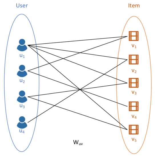
Figure 1. An example of bipartite graph $G=\left(U,V,E\right)$, which has two types of entities $U$ and $V$. The edges between the two entities are entitled with weights $W_{UV}$, meaning the user watches and rates the movie.

However, most graph embedding algorithms focus on either homogenous networks such as Node2vec [12] or knowledge graphs such as Trans series [13,14], only a few existing works focus on bipartite graphs [15,16,17,18,19].

There are two challenges when embedding bipartite graphs:

• The first challenge we address is to leverage both the characteristic of bipartite graphs and the auxiliary information. In bipartite graphs, only the structure information is presented by the relations between users and items. Through incorporating both the content information and the bipartite graph structure, we can improve not only the model accuracy but also the cold-start problem.
• Both homogenous and heterogeneous network algorithms take into account the explicit relations between two types of vertices. However, there are implicit relations between the same type of vertices in bipartite graphs. For example in Figure 1, where $U$ and $V$ are two sets of vertices with different types, E is the set of edges, labeled with weights $W_{uv}$. The edge can represent the interaction between user $U$ and item $V$, for example the rating that a user gives to an item. Suppose it is a user-movie graph. User 1 and user 2 should have an implicit relation as they share the same interest in movie 1. When embedding those users into low-dimensional spaces, they should be neighbors with similar vectors, thus more likely to be recommended to the same preferred movies. As discussed in [20], modeling both relation types will improve the recommendation accuracy.

A recent work by Berg et al. [18] proposed graph convolutional matrix completion (GC–MC) for embedding the bipartite graph within a graph-based autoencoder framework, which produces the user and item embedding through a form of message passing algorithm. However, GC–MC focused on the interaction between users and items, i.e., the explicit relation in the bipartite graph, yet the implicit relation has not been captured.

Thus, inspired by the previous work of graph embedding techniques, we propose attentive implicit relation recommendation incorporating content information (AIRC), which is an extended GC–MC model with an implicit-relation embedding attention mechanism built-in for the bipartite graph. Our main contributions are as follows:

• We define the user implicit relation graph the same way we define the item implicit relation graph, as where users are linked if they have relations to the same item in the bipartite graph. As a result, similar users/items become neighbors. In order to preserve the similarity during embedding, we resort to the solution of graph attention mechanisms such as graph attention networks (GATs) [21]. GAT is based on graph convolution algorithms, which leverages features of neighbors from a node by learning different weights of different neighbors. Thus, the implicit relations are preserved by embedding similar nodes with close vectors.
• We incorporate content information in our framework. We train both user and item features through a simple CNN, yields user and item feature vectors. Then we represent each node in the user graph and item with the feature vectors, so that nodes with similar feature vectors can affect each other more in a neighborhood during the GAT process and also reduce the problem of a cold-start.
• With the user–item bipartite graph, we add a graph attention layer into GC–MC as side information, and trained together to obtain the final embedding of each user and item. The structure of our framework is shown in Figure 2. A bipartite graph is reconstructed into user and item implicit relation graphs, and through a simple CNN operation we obtain a pretrained feature matrix. Those matrices are then fed into a graph attention mechanism applied on the implicit graphs, whereby becomes side information and trained together with GC–MC algorithm. The structure will be in detail explained in Section 3.
  

  Figure 2. The structure of our framework attentive implicit relation recommendation incorporating content information (AIRC). The bipartite graph is reconstructed into the user implicit relation graph and item implicit relation graph. Then CNN process pretrained user and item feature matrices, which is the input of graph attention mechanism applied on implicit relation graphs as an extended layer of GC–MC.

Our proposed AIRC framework was evaluated on the Movielens dataset. Experiments showed that our framework outperforms previous works in terms of link prediction and recommendation, evaluated by root mean square error (RMSE). Moreover, we also demonstrate that our framework can achieve better results more quickly compared with others.

The paper is organized as follows: we first demonstrate related work in Section 2. Then we represent our framework in details in Section 3. In Section 4 we will explain experimental setup and discuss the results. Finally, we will make a conclusion of our work and introduce some future works in Section 5.

2. Related Work

Many techniques have been put forward in the fields of recommendation systems. One traditional approach is matrix factorization (MF), which map users and items into latent factor, and then high correspondence regards to recommendation [22,23]. In most cases, traditional approaches such as MF are integrated into neural networks. Dziugaite and Roy proposed neural network matrix factorization to construct user and item latent features through a multilayer feed-forward neural network, and then optimized the features by alternating between user and item networks [24]. DeepFM [25] integrates the deep neural network into FM, which captures the linearity and the non-linearity interactions between features.

Besides, neural networks CNN/RNN are also used in recommendation. Devooght et al. presented to make a session based recommendation by RNN, leveraging between both long and short memory by adding noise to the training history sequences [5]. Zheng et al. [26] proposed DeepCoNN that used two parallel CNNs to approximate the behavior of users and the properties of items. The key idea is to extract the review text into a low-dimensional embedding space. Moreover, autoencoders are also applied in recommendation systems. AutoRec [27] is a successful algorithm that combines collaborative filtering with autoencoders. It takes partial user and item vectors as input and reconstructs them in the output layer. CDL [22] proposed a Bayesian network that integrates a denoising autoencoder with MF, which balanced the interaction history of users and items and the side information.

With the growth of the attention mechanism, one could use the attention mechanism together with neural networks to filter out unimportant information to make better recommendation [28]. Zheng et al. came up with the memory attention aware recommendation system that learned the behavior of users by facilitating CNN with an attention part to memorize their most interested items [29]. Ying et al. [30] proposed a hierarchical model for the attention mechanism. Different from other sequential recommendation, this algorithm created two attention networks designed for short- and long-term interactions respectively.

Currently, there is an increasing trend that data are represented as graphs. Graph embedding becomes a popular alternative to recommendation systems. Sperduti et al. [31] motivated early studies on GNNs and then Gori et al. [32] came up with the definition of graph neural networks. Many algorithms learn the embedding and the graph structure by propagating node features until equilibrium has reached. GraphSage [33] proposed by Hamilton et al. adopts sampling a fixed-size neighbor for each node and distributing the neighbors’ features to the whole graph. PGE [34] further optimized the sampling procedure of GraphSage. PGE assigns different weights to the neighbors of a node according to their feature similarity, and then aggregates the sampled neighbors feature with a biased neural network. Moreover, previous deep learning algorithms were integrated into graph embedding. GraphRNA [35] combined random walks based on node attributes and graph recurrent networks. GAT [21] and GAM [36] adopts the self-attention mechanism to mark the different influence of node neighbors.

Bipartite network is a special heterogeneous network that emphasizes on the interaction between users and items. Co-Hits algorithm [37] was proposed to solve the query-URL graphs, which leveraged content information and also the graph structure. BiNE [19] developed bipartite network embedding methods by performing random walks on the implicit relations and optimizing together with explicit relations. Hu et al. [38] focused on the collaborative filtering in bipartite graphs. GC–MC [18] utilized graph autoencoder into bipartite graphs by modeling the message passing procedure between user and item, however, content information is not fully integrated. Recently, Wang et al. proposed KGAT [39], which recursively propagates a node embedding and attends over its neighbors by attention mechanism in collaborative knowledge graphs.

Our framework is an enhanced work on GC–MC [18], considering the recommendation problem as matrix completion. However, we focus on the implicit relations in bipartite graphs, which shows great similarity information about vertices of the same type. Besides, different from the work BiNE [19] that performs random walks on the implicit relations, we adopt the attention mechanism that combines content information with the implicit relation, and emphasize on the important features and neighbors.

3. Proposed Work

In this section, we described our proposed framework AIRC. The key idea is to aggregate the implicit relation and also the context information into the embedding process of bipartite graphs. We first introduce the generation of implicit relation graphs, integrated with feature information. Then we present the GC–MC based model with an additional attention layer that leverages the implicit relation graph.

To begin with, we denote a bipartite graph $G=\left(U,V,E\right)$ and its weight matrix $W$, where $U$ and $V$ denote two types of vertices respectively, $E\in U\times V$ represents the edges between $U$ and $V$. Each edge carries a weight $w_{ij}$ that represents the connection strength between the two vertices $u_i$ and $v_j$. As shown in Figure 3a, $u_i$ and $v_j$ denote the $i$-th and $j$-th vertices in $U$ and $V$, where $i\in \left\{1,2\dots \left|U\right|\right\}$, $j\in \left\{1,2\dots \left|V\right|\right\}$.

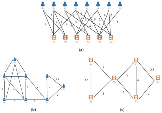
Figure 3. A demonstration of the reconstruction of a bipartite graph $G=\left(U,V,E\right)$ end edge weights $W$ in (a). The 1st-order implicit graphs are shown in (b,c) according to Definition 1 and the weights are calculated with Equation (1).

3.1. Implicit Relation Graph Generation

As illustrated above, a bipartite graph contains both explicit relations and implicit relations. Explicit relations usually reveal the interaction between different types of entities, for instance actors perform movies, users purchase goods and then rate them. Previous work shows a lot of effort in preserving the information in the explicit relations, such as random walks, whereby vertices are nearby in the projecting space if they are strongly connected. However, in the bipartite graph, implicit relations exist between the same type of entities. The semantics of these implicit relations should also be preserved in order to recommend with higher precision.

We proposed to divide the bipartite graph $G$ into two homogenous networks $G_U$ and $G_V$, for two types of vertices respectively. Those homogenous networks contain the information of implicit relations. In order to comprehend, we first defined the k-order implicit relation graph:

Definition 1.

Given a bipartite graph $G = \left(U,V,E, W\right)$ with two types of vertices $U$ and $V$, edges $E\in U\times V$, and weights $W$, we define k-implicit relation graph $G_N^k=\left(N, R_N\right)$ with weight matrix $L$, where $N$ can be either $U$ or $V$, and $R_N\in \left(R_U, R_V\right)$, where $R_U\in U\times U$ and $R_V\in V\times V$. We define $r_{u_i,u_{i^{\prime }}}\in R_U$ and $r_{v_j,v_{j^{\prime }}}\in R_V$ if there exist shortest paths $P$ with k-order between vertices ($u_i,u_{i^{\prime }}$) and ($v_j,u_{j^{\prime }}$) in the bipartite graph $G$ respectively, where $i, i^{\prime }\in \left\{1,2\dots \left|U\right|\right\}$, and $j, j^{\prime }\in \left\{1,2\dots \left|V\right|\right\}$. The weight matrix $L$ can be calculated with different functions $L_U^k=F(w_{im},w_{i^{\prime }m}|m\in V and m\in p)$ or $L_V^k=F(w_{jm},w_{j^{\prime }m}|m\in U and m\in p)$, where $m$ is the middle vertex in the shortest path $p$.

However, constructing a higher order path between vertices is unfeasible especially for large networks, as the complexity is exponential. Thus, in order to reach the balance between the complexity and effectiveness, we only used a 1st-order implicit relation graph. For the reason that the 1st-order path already preserves most of the neighbor information, and with the help of the graph attention algorithm, higher-order implicit relation can also be learned as will be explained in Section 3.2. To simplify, we used $G_U$ and $G_V$ to represent the 1st-order graph.

Furthermore, in order to preserve the semantics of the weight information, we defined a weight function in the implicit relation graph:

$$F\left(L\right)=\frac{{{\displaystyle \sum }}_{m\in V,m\in p}\left(C-\left(w_{u_i,m}-w_{u_{i^{\prime }},m}\right)\right)}{S}$$

(1)

where $S$ is the number of shortest paths $p$ between $u_i$ and $u_{i^{\prime }}$ and $C$ is the maximum value of weight matrix $W$. This weight function represents the similarity between the same type of vertices. For example, two users have similar taste when they see the same movies and also rate similarly. When two users rate the same movies however with a large difference among the ratings, we argued that their tastes differed, and the weight value was small, thus their embeddings were far from each other.

Figure 3a shows a user–movie bipartite graph $G$, where edges represent the rating action from users $U$ to movies $V$. According to Definition 1, we constructed the user implicit graph $G_U=\left(U,R_U\right)$ shown in Figure 3b, and item implicit graph $G_V=\left(V, R_V\right)$ shown in Figure 3c. To illustrate, in Figure 3b the edge $r_{u_1,u_2} \in \left(u_1,u_2\right)$ demonstrates that in Figure 3a a shortest path with 1st-order exists between vertices $u_1,u_2$. Additionally, $l_{u_1,u_2}$ is calculated from the two shortest paths between vertices $u_1,u_2$, namely $u_1\to v_1\to u_2$ and $u_1\to v_2\to u_2$. Additionally, graphs $G_U^1$ and $G_V^1$ preserve the semantics of original bipartite graph $\mathrm{G}$. For instance, in (b) the edge $r_{u_1,u_2}$ represents that users $u_5,u_7$ have rated the same movie $v_5$, and the weight $l_{u_5,u_7}=5$ is large, meaning that they share the same taste. As a result in the embedding space they become neighbors, and with the later application of graph embedding techniques their projections will be similar, thus raising the recommendation accuracy.

3.2. Content Information Extranction

Despite the structure information of the bipartite graph, we also leverage content information C to embed vertices so that each vertex has its own feature vector. In this paper, we used Movielens dataset to evaluate the framework. On one hand, following the work of [40], we used a CNN to learn the feature matrix of both users and movies. On the other hand, with the help of obtained feature vectors, we employed the graph attention mechanism correspondingly so that the hidden information attends over its neighbors. The purpose of CNN is to obtain initial feature matrices, which can reduce the cold-start problem for the graph attention mechanism. With the pretrained feature matrices as input, the graph attention mechanism attends the hidden features more quickly.

3.2.1. CNN Process

As shown in Figure 4, the network is composed of two parts: the user network and movie network. This process involves three types of features: single-value, multi-value and text-type. The first layer for both the user and movie network is the embedding layer. For the single-value feature, such as user/movie ID, user gender, user age and user occupation, we embed the features into numbers (for instance, age is categorized into 7 groups according to the age range according to Table 1, and gender is represented as 0 for female and 1 for male); for movie genres, which is multivalued, meaning that it can be comedy and romance at the same time. There are totally 18 types, so we set a genres index vector, where 0–18 are used to represent each type including the vacant value; for the text-type feature, i.e., movie titles, according to statistics [40], no more than 5216 words in the movie titles and the length is within 14 words. So, we transformed the movie titles into a 15 (14 + 1)-bit index vector with numbers from 0 to 5216.

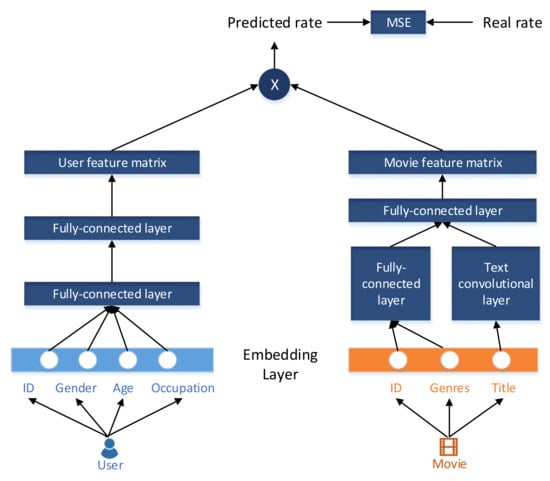
Figure 4. A CNN process to extract the initial feature matrix of users and movies. The user features are extracted by two fully connected layers. The movie titles are processed by a text convolutional layer, and by a fully connected layer, the movie features are extracted. Finally a multiply operation and optimization are conducted.

Table 1. The categorization of the user feature age.

Age	Encode
Under 18	1
18–24	18
25–34	25
35–44	35
45–49	45
50–55	50
Over 56	56

Next step we divided the network into two parts to illustrate in detail. In the user network we use two fully connected layers to extract the user features. The first layer embeds different features into the same dimension $1\times 128$ as follows:

$$f_i=Relu\left(C_i\times k_{1i}+b_{1i}\right)$$

(2)

$$f_{u\_dense1}=f_{uid}\oplus f_{gender}\oplus f_{age}\oplus f_{uoccupation}$$

(3)

where $i$ is the corresponding feature name, $C_i$ is the input feature matrix, $k_i$ is the kernel and $b_i$ is the bias. We used Equation (2) to calculate $f_{uid},f_{gender},f_{age} \mathrm{and} f_{uoccupation}$. Then we concatenated those hidden representations as shown in Equation (3). The second fully connected layer was used to embed the user features with dimension $1\times 200$, to be in the same space as in the movie feature network, shown in Equation (4):

$$f_{u\_dense2}=Tanh\left(f_{u\_dense1}\times k_2+b_2\right)$$

(4)

On the other hand, in the movie network, movie title features were extracted using the concept of natural process and text convolution networks [41]. As shown in Figure 5, we first transformed the words into word vectors. Suppose a sentence contains $n$ words represented as the $d$-dimensional word vector. Thus the sentence can be represented as Equation (5):

$$x_{1:n}= x_1\oplus x_2\oplus \dots \oplus x_n$$

(5)

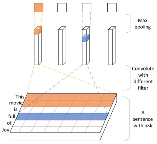
Figure 5. The text convolution layer that extract the important features of movie titles. A sentence is convoluted with different sizes of kernel, and by max-pooling operation, important features are extracted.

In order to extract the features, we used a convolution filter $w\in R^{hk}$ applied to a window of $h$ words. Thus a feature $c_i$ was calculated using Equation (6):

$$c_i=Tanh\left(w ·x_{i:i+h-1}+b\right)$$

(6)

The dimension of this convolution filter varies with each possible window of words to generate a feature map:

$$c=\left[c_{1, }{c}_{2, }\dots , c_{n-h+1}\right]$$

(7)

To address the problem of capturing the most important feature in the sentence, we used a max pooling operation for each window size:

$$\widehat{c}=maxpool\left(c\right)$$

(8)

Then after a dropout operation, we got the features of movie titles $f_{titles}$. Meanwhile, using Equation (2) $f_{vid} \mathrm{and} f_{genres}$ were obtained. Afterwards, the same as the user network, we concatenate each movie hidden representation and applied a fully connected layer, resulting in a feature vector with dimension $1\times 200$.

$$f_{v\_dense1}=f_{vid}\oplus f_{genres}\oplus f_{titles}$$

(9)

$$f_{v\_dense2}=Tanh\left(f_{v\_dense1}\times k_2^{\prime }+b_2^{\prime }\right)$$

(10)

To obtain the feature vectors, we multiplied the above user and movie networks results and regress with the real ratings, then optimize loss with MSE. After pretraining, we could obtain a user/movie node, which is represented by feature matrices $f_u \mathrm{and} f_v$, and then leveraged in the attention mechanism explained in Section 3.2.2.

3.2.2. Attention Mechanism

Currently, the attention mechanism has been widely used in many deep learning areas. Integrated into different neural networks, one of the benefits of the attention mechanism is dealing with a sparse and large dataset by focusing on the important information, just like the human visual attention mechanism [42,43,44].

Inspired by the work of the Google team [45] and graph attention mechanism [21], we deployed a self-attention mechanism and multiheaded attention to handle the feature matrix $f_u \mathrm{and} f_v$.

Compared with the normal attention mechanism, self-attention learns the hidden representation of a node by attending over its neighbor, instead of attending all the nodes in the graph, which both increase the efficiency and become more attentive on the similar nodes.

Suppose we had the user implicit graph $G_u$, item implicit graph $G_v$ according to Definition 1, users with the same interest on items become neighbors. Considering the attention mechanism as a neural network layer, our aim is to get the representation of the next layer through hidden representation. Take the user graph as an illustration, a user node is represented as $n_i=\left\{f_{i1},f_{i2}\dots f_{iF}\right\}$, where $F$ is the number of features. Figure 6 and the following equations describe the update procedure of node features from layer $l$ to layer $l+1$. The output of layer $l+1$ has the form of $n_i^{\left(l+1\right)}\in R^{F^{\prime }}$.

$$z_i^{\left(l\right)}=W^{\left(l\right)}{n}_i^{\left(l\right)}$$

(11)

$$e_{i{i}^{\prime }}^{\left(l\right)}=LeakyRelu({\overrightarrow{a}}^{{\left(l\right)}^T}(z_i^{\left(l\right)}\Vert z_{i^{\prime }}^{\left(l\right)}))$$

(12)

$$a_{i{i}^{\prime }}^{\left(l\right)}=\frac{exp\left(e_{i{i}^{\prime }}^{\left(l\right)}\right)}{{{\displaystyle \sum }}_{k\in N}\exp \left(e_{ik}^{\left(l\right)}\right)}$$

(13)

$$n_i^{\left(l+1\right)}=sigmoid\left({{\displaystyle \sum }}_{i’\in N}{a}_{i{i}^{\prime }}^{\left(l\right)}{z}_{i^{\prime }}^{\left(l\right)}\right)$$

(14)

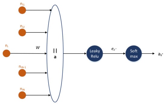
Figure 6. The attention layer on the user implicit graph. A node $n_i$ and its neighbors are represented with an orange circle. The operation $\Vert$ represents the concatenation. Then we apply LeakyRelu and Softmax operation to obtain the attention score $a_{i{i}^{\prime }}$.

Equation (11) shows the embedded procedure of node $n_i^{\left(l\right)}$, where $W^{\left(l\right)}\in F\times F^{\prime }$ is a trainable weight vector. Equation (12) is the original attention score between a node and its neighbors $n_{i^{\prime }}$. We first concatenated two embedded vector $z$, and multiplied it with a trainable weight vector ${\stackrel{\rightharpoonup }{a}}^{\left(l\right)}\in R^{2\times F^{\prime }}$, finally apply a LeakyRelu activation function. Then we computed the Softmax operation of the original attention score by Equation (13). Lastly Equation (14) denotes the update rule, which calculates the weighted sum of all the neighbor features. Whereby, we defined two trainable weights, namely $a, W$. To illustrate this further, the weight $W$ denotes the weight to emphasize the important features of a given node, while on the other hand $a$ emphasizes the different influence of the neighbor on a given node. Therefore, we see that the graph attention mechanism adopts attention operation to replace the generalized constant in the graph convolutional network.

Additionally, we used multihead attention to enrich the ability of the model and to stable the process of training. The main inspiration of multihead attention is to linearly project the hidden representation into different subspace, where each subspace has different reflection feature distribution information. Then those projections are concatenated and once again embedded shown as Equation (15).

$$n_i^{\left(l+1\right)}=|{|}_{k=1,\dots ,K}sigmoid\left({\displaystyle \sum }_{i\in N}{a}_{i{i}^{\prime }}^k{W}^k{h}_{i^{\prime }}^{\left(l\right)}\right)$$

(15)

where $k$ represents the number of attention head.

To summarize, we extracted the context information by a CNN network and integrated into the graph attention mechanism for users and items separately. The benefit of this procedure is that we took not only a node’s features into consideration but also its neighbor’s feature, whereby the node embeddings are feature-oriented and neighbor-alike, in order to increase the recommendation accuracy. In Section 3.3, we added this attention layer as content information into the whole structure and trained together with the GC–MC model.

3.3. Structure

As a ubiquitous heterogeneous graph, bipartite graphs have drawn much attention because of their ability to model the relationship between two kinds of entities. Traditional graph embedding algorithms such as random walks, the graph convolutional network (GCN) for homogenous networks cannot be directly carried out on bipartite graphs. The essential purpose of GCN is to extract the spatial features of topological graphs, which uses a convolutional kernel to embed nodes and then propagates the node information to all the graphs. It is trivial to notice that the propagation process is a message passing process [46], which happens to be the nature of bipartite graphs.

However, due to the heterogeneity in bipartite graphs, the message passing should be divided into two parts: each type of the vertex correspondingly. As a solution, the paper [18] proposed the graph convolutional matrix completion (GC–MC). The main idea is to use the graph autoencoder and GCN to obtain user and item embeddings by the inspiration of message passing separately. Then with a bilinear decoder the recommendation task is accomplished by the means of matrix completion.

In this paper we used GC–MC as the basis, adding feature extraction and the graph attention layer as content information, and trained together to embed the bipartite graphs in order to make a recommendation. The whole structure is shown in Figure 2.

As a basis, the task of GC–MC is to learn the explicit relation between users and the item through message passing. A user’s embedding is the gathering of messages from the items that it interacts with, which was accomplished by a GCN layer. Suppose we had a bipartite graph $G=\left(U,V,E\right)$, the initial user embedding $h_{u_i}$ revealing the implicit relation is shown by Equation (16):

$$h_{u_i}=\sigma [|{|}_{r\in R}({{\displaystyle \sum }}_{v_j\in N_i}{\mu }_{v_j\to u_i,r})]$$

(16)

where ${\mu }_{v_j\to u_i,r}$ is the message passing from item $v_j$ to user $u_i$ under the edge type $r$ with the form ${\mu }_{v_j\to u_i,r}=\frac{1}{c}{W}_r{x}_{v_j}$, $c$ is the regularization constant and $N_i$ is the neighbors of user $u_i$. The operator $\Vert$ is concatenation and $\sigma$ is activation function such as LeakyRelu.

After modeling the explicit relation, we added a graph attention layer to combine the content information and implicit relation as illustrated Section 3.2. With the implicit relation graph $G_u \mathrm{and} G_v$ and the pretrained feature matrix $f_u \mathrm{and} f_v$, we used Equation (5) to get the side information $n_i,n_j$. Then we integrated the initial embedding $h_{u_i}$ together with the side information $n_i$ into a dense layer as shown in Equation (17):

$$u_i=\sigma \left(W{h}_{u_i}+W_2{n}_i\right)$$

(17)

where $W$ and $W_2$ are trainable parameters. Thus, we obtained the embedding matrix of users, and the items embedding in the same way, where users and items share the same weight $W$. The procedure to get the embedding for item $v_j$ is the same as the user illustrated above.

In order to train and recommend, a decoder was performed to estimate the possibility distribution of getting a certain rate by a Softmax operator.

$$p\left({\widehat{y}}_{ij}=r\right)=\frac{e^{u_i^T{Q}_r{v}_j}}{{{\displaystyle \sum }}_{t\in R}{e}^{u_i^T{Q}_t{v}_j}}$$

(18)

where $Q$ is also a trainable parameter. Then the predicted rating was calculated:

$${\widehat{y}}_{ij}={\displaystyle \sum }_{r\in R}rp\left({\widehat{y}}_{ij}=r\right)$$

(19)

For the training phase, our goal was to minimize the equation below, where $I$ equals to 1 when r and ${\widehat{y}}_{ij}$ are the same, equals to 0 otherwise.

$$L={\displaystyle \sum }_{r\in R}I\left(r= {\widehat{y}}_{ij}\right)\log p\left({\widehat{y}}_{ij}=r\right)$$

(20)

In summary, the Algorithm 1 integrates both the implicit relation and the explicit relation in bipartite graphs, and takes content information into consideration as follows:

Algorithm 1. Attentive implicit relation recommendation incorporating content information (AIRC).

Input: Bipartite graph $G=\left(U,\hspace{1em}V,\hspace{1em}E\right)$, content information $C_u$ and $C_v$ Output: Embeddings $u_i$ and $v_j$, prediction ${\widehat{y}}_{ij}$ 1: Partition $G$ into $G_u$ and $G_v$ according to Def. 1 2: user feature matrix $f_u=CNN\left(C_u\right)$ 3: item feature matrix $f_v=CNN\left(C_v\right)$ 4: for i = 1,…, max_iter do 5: GCN layer: user initial embedding:              $h_{u_i}\leftarrow \sigma [|{|}_{r\in R}({{\displaystyle \sum }}_{v_j\in N_i}{\mu }_{v_j\to u_i,r})]$       Item initial embedding:              $h_{v_j}\leftarrow \sigma [|{|}_{r\in R}({{\displaystyle \sum }}_{u_j\in N_i}{\mu }_{u_i\to v_j,r})]$ 6: Attention layer              $n_i\leftarrow \left\{f_{i1},f_{i2}\dots f_{iF}\right\}$               $z_i^{\left(l\right)}\leftarrow W^{\left(l\right)}{n}_i^{\left(l\right)}$              $e_{i{i}^{\prime }}^{\left(l\right)}\leftarrow LeakyRelu({\overrightarrow{a}}^{{\left(l\right)}^T}(z_i^{\left(l\right)}||z_{i^{\prime }}^{\left(l\right)}))$              $a_{i{i}^{\prime }}^{\left(l\right)}\leftarrow \frac{exp\left(e_{ii\prime }^{\left(l\right)}\right)}{{{\displaystyle \sum }}_{k\in N}\exp \left(e_{ik}^{\left(l\right)}\right)}$ User attentive embedding:              $n_i^{\left(l+1\right)}\leftarrow sigmoid\left({{\displaystyle \sum }}_{i^{\prime }\in N_i}{a}_{i{i}^{\prime }}^{\left(l\right)}{z}_{i^{\prime }}^{\left(l\right)}\right)$ Item attentive embedding:              $n_j^{\left(l+1\right)}\leftarrow sigmoid\left({{\displaystyle \sum }}_{j^{\prime }\in N_j}{a}_{j{j}^{\prime }}^{\left(l\right)}{z}_{j^{\prime }}^{\left(l\right)}\right)$ 7: Dense layer: user hidden representation:              $u_i\leftarrow \sigma \left(W{h}_{u_i}+W_2{n}_i^{\left(l+1\right)}\right)$       item hidden representation:              $v_j\leftarrow \sigma \left(W{h}_{v_j}+W_2{n}_j^{\left(l+1\right)}\right)$ 8: Decoder: $p\left({\widehat{y}}_{ij}=r\right)=\frac{e^{u_i^T{Q}_r{v}_j}}{{{\displaystyle \sum }}_{t\in R}{e}^{u_i^T{Q}_t{v}_j}}$ rate prediction:              ${\widehat{y}}_{ij}\leftarrow {\displaystyle \sum _{r\in R}}rp\left({\widehat{y}}_{ij}=r\right)$ 9: Train phase: $L={\displaystyle \sum }_{r\in R}I\left(r={\widehat{y}}_{ij}\right)\log p\left({\widehat{y}}_{ij}=r\right)$       update parameter ${\stackrel{\rightharpoonup }{a}}^{\left(l\right)},W^{\left(l\right)},W,W_2$ by gradient descent minimizing L 10: end for

According to the algorithm, we first reconstructed the bipartite graph into $G_u$ and $G_v$. Then step 2 and 3 were obtained by Equations (2)–(10), so that we had the initial user and item feature matrices in the CNN process. Next, we added an additional graph attention layer shown as step 6, which operated on $G_u$ and $G_v$ with the pretrained input $f_u$ and $f_v$. Finally we trained the attention layer together with GC–MC from step 5 to step 8 by minimizing the loss $L$ iteratively.

4. Experiment

In this section we evaluated our framework AIRC on the dataset Movielens, which contains users, items and their content information as well as ratings, which exactly corresponds with our needs.

4.1. Dataset

Movielens is a widely used benchmark for movies, collected by Grouplens Research. More information can be seen from the Movielens official website (https://grouplens.org/datasets/movielens/). In this experiment, we mainly used two datasets from Movielens, 100K and 1M. The statistics are shown in Table 2.

Table 2. The statistic of the dataset Movielens.

Dataset	Items	Users	Ratings	Density
Movielens-1M	3706	6040	1,000,209	0.0447
Movielens-100K	1682	943	100,000	0.0630

Dataset description: Movielens-100K is the movie dataset with over 100,000 ratings. It contains 943 users and 1682 movies. On the other side, Movielens-1M collects 1 million ratings from 6040 users on 3900 movies. However, after screening those users without valid ratings, only 3706 users are left to be put in use. For both datasets, we transformed the rating files to construct the bipartite graphs, consequently constructing the implicit relation graphs. Additionally, they also contained the user profile and movie profile, which we took as content information and then were fed into our CNN layer and given attention weights.

Preprocessing: For the user profile, we only used UserID, gender, age, and occupation attributes to describe users. Firstly, we encoded 0 for female and 1 for male. Then we categorized age into 7 groups, and occupation into 21 types, then encoded them as listed numbers. For the movie profile, we used MovieID, genres and title attributes, where genres had 18 types and were encoded into listed numbers. The handling for titles was different from other attributes: we first created the dictionary from the text to numbers, and converted the description of the text into a list, then with the help of text convolutional neural networks as illustrated in Section 3.2.1, we obtained the title feature representation.

Implicit relation graphs (IRG): According to Definition 1, we constructed the user and movie implicit relation graph. The statistic is summarized in Table 3. We could see that with the first order shortest path, we already had over 9 million edges for Movielens-1M dataset, not to mention this number of edges was proportional to the number of orders of shortest path. That is why we only used the first order shortest path to construct implicit relation graphs.

Table 3. The statistic of the reconstructed implicit graphs.

Dataset	Graph	No. Nodes	No. Edges
Movielens-1M	User IRG	3706	9,469,555
	Item IRG	6040	32,721,414
Movielens-100K	User IRG	943	859,323
	Item IRG	1682	1,574,374

4.2. Baseline

As our framework improved the recommendation based on GC–MC algorithms, we compared our results mainly with GC–MC. Additionally, for movielens-100k, we compared the results with matrix completion algorithms, and for movielens-1M, we compared our results with recommendation algorithms cooperated with collaborative filtering algorithms.

GC–MC [18]: it is a graph autoencoder framework designed for bipartite graphs. The main idea is to learn the user and item representation by message passing. In this comparison experiment, we set dropout as 0.7 and layer size as $\left[500, 75\right]$ in the GCN layer. For Adam, we set the learning rate 0.01. We adopted $batch\_size= 50$ for Movielens-100K and $batch\_size=100$ for Movielens-1M.

MC [47]: it is a classic matrix completion method. It aims to recover the low-rank matrix.

GMC [48]: Geometric Matrix Completion (GMC) improves the matrix completion by constraining the solution to be smooth. It combines the content-based filtering with clustering techniques. Additionally, the entries are set to $500\times 500$ for Movielens-100K.

sRGCNN [49]: Separable recurrent multi-graph CNN (sRGCNN) used geometric deep learning to solve the problem of matrix completion. The architecture contains a CNN for spatial feature learning and LSTM matrix diffusion. The parameter settings are as follows: Chebyshev polynomials of order $p = 5$, output $dimension=32$, LSTM cells with 32 features and $T = 10$ diffusion steps.

PMF [23]: Probabilistic matrix factorization (PMF) aims to solve the problem of large dataset with few ratings, especially the dataset that is sparse and unbalanced. The feature dimension is set to 60 as it performs the best.

U-AutoRec [27]: The model proposed to combine the collaborative filtering algorithm with an autoencoder. We used a single hidden layer architecture and the number of hidden units is set to 500 and the learning rate as 0.001.

NNMF [24]: Neural network matrix factorization (NNMF) focused on the improvement on matrix factorization by replacing the inner product by a neural network, so that the inner product and latent representation are tailored for a different dataset. We set feature dimension as 60 and the learning rate as 0.005.

4.3. Evaluation Metrics

We used root mean square error (RMSE) as our evaluation:

$$RMSE=\sqrt{\frac{{{\displaystyle \sum }}_{i=1}^S{\left(r_i-\widetilde{r_i}\right)}^2}{S}}$$

(21)

where $r_i$ is the real world rating for item $i$, $\widetilde{r_i}$ is the predicted value and S is the total number of rating.

4.4. Results and Discussion

In this section, we tested our framework AIRC with state-of-art algorithms.

Our experiment environment was Aliyun with 8 vCPU, 32 GiB, Intel Xeon Platinum processor. To show the improvement of our framework, we used the same parameter setting as in GC–MC, i.e., batch_size = 50 for Movielens-100K, and batch_size = 100 for Movielens_1M, drop_out = 0.7, additionally we collaborated features in our attention layer, and we set the dimension of hidden feature to 8, attention_head = 8.

Movielens-100K:

We first evaluated the performance on Movielens-100k as shown in Table 4.

Table 4. Root mean square error (RMSE) for Movielens-100K. The result of baseline matrix completion (MC), GMC and sRGCNN is taken from [49].

Algorithm	RMSE
MC	0.973
GMC	0.996
sRGCNN	0.929
GC–MC (with features)	0.910
AIRC (Ours)	0.892

We can see that among the traditional matrix completion algorithms, our framework performed the best with the least RMSE. GMC performed better than MC because GMC was better at handling sparser dataset like Movielens-100K. sRGCNN improved the result by the usage of neural networks that extracted the features of users and items. Compared with the traditional matrix completion algorithm MC, our framework improved the performance by 8.32%. We can see that our framework improved the results of GC–MC, because we incorporated implicit relation and content information of users and items, which have deep influences during the recommendation. One thing to notice is that GC–MC reached its best performance at epoch 89, however our algorithm reached the best at epoch 50. The reason is that in the first step we already trained the feature vector with CNN, plus the attention mechanism, thus our framework made more use of the content information.

Movielens-1M:

In the above experiment, we compared our framework with matrix completion algorithms. So, for Movielens-1M, we used another type of recommendation algorithms as our baseline: collaborative filtering algorithms. The result is shown in Table 5. The algorithm AutoRec combines the autoencoder with collaborative filtering that reconstruct users and items in the output layer. It had a better result than PMF. NNMF added neural networks based on MF, which is capable of dealing non-linearity in the dataset. Compared with other matric factorization algorithms and collaborative filtering algorithms, our framework outperformed and improved RMSE compared with GC–MC by 1.32%. The improvement was not as obvious as Movielens-100K, as the data was much sparser than Movielens-100K. However, with the rich information provided by content information and the implicit relation among the same type of entities, our framework was more effective.

Table 5. RMSE for Movielens-1M. The result of baseline probabilistic matrix factorization (PMF), U-AutoRec and NNMF is taken from [22].

Algorithm	RMSE
PMF	0.883
U-AutoRec	0.874
NNMF	0.843
GC–MC (with features)	0.832
AIRC (Ours)	0.821

Cold-start Analysis:

As illustrated before, our framework reached the best RMSE at the earlier stage, i.e., relieving the problem of cold-start. As shown in Figure 7a,b, compared with GC–MC, our framework had less RMSE at the start and smoothly reduced, especially for Movielens-100K, which had a smaller network structure. At the start, our framework reduced to 4.7% RMSE for Movielens-1M, and reduced to 8.0% RMSE for Movielens-100K. Besides, a bigger gap occurred as the epoch increased. We can see that at epoch 9, the difference increased to 14.7% compared with the start point for Movielens-1M. So, we could conclude that our framework not only reduced the cold-start problem at the beginning but also reached the best result more quickly.

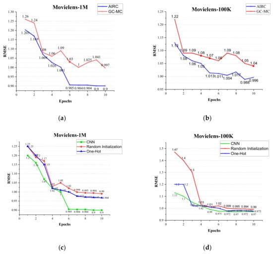
Figure 7. (a) The cold-start comparison of dataset Movielens-1M between our framework and GC–MC; (b) the cold-start comparison of dataset Movielens-100K between our framework and GC–MC; (c) the cold-start comparison of dataset Movielens-1M among the original pretrained user and item feature matrices, random initialized feature matrices and one-hot feature matrices and (d) the cold-start comparison of dataset Movielens-100K among the original pretrained user and item feature matrices, random initialized feature matrices and one-hot feature matrices.

Moreover, in order to show the effectiveness of the CNN part in our framework, which aims to reduce the problem of cold-start, we set up an ablation experiment and the result is shown in Figure 7c,d. Instead of pretrained $f_u,f_v$ that fed into the graph attention mechanism, we set two comparison experiments, namely random initialized and one-hot initialized user and item matrices, which were fed into the graph attention mechanism.

We can see from Figure 7c,d that the impact of initializing the user and item feature matrices differed in the same task: (1) our framework that incorporates CNN to process the features performed best when dealing with the cold-start problem, as the features were pretrained. Take dataset Movielens-100K for example, AIRC-CNN have already reached a RMSE with 1.13, which was 30% less than AIRC-RandomInitialzation and 6% less than AIRC-OneHot. Besides, the curve of AIRC-CNN was smoother and less than those two algorithms; (2) our framework that incorporated one-hot for feature processing performed better than that of random initialization. The reason is that one-hot initialization takes real-world features into consideration, rather than completely randomized. However, our framework, no matter how the feature matrices were initialized, started with a smaller RMSE and reduced quickly compared with GC–MC.

Thus, we could see that with the pretrained feature matrix, through the graph attention mechanism that mined the implicit relations in the bipartite graphs, our framework improved the effectiveness compared with GC–MC and relieved the problem of the cold-start.

5. Conclusions

In this paper, we presented AIRC, a GC–MC based framework, which learns the implicit relation and content information in bipartite graphs. We reconstructed the bipartite graphs into implicit relation graphs and adopted the graph attention mechanism. The reconstructed implicit relation graph contained the same entity type, which was linked if there existed the shortest path between them in the bipartite graph. Besides, we used a CNN to pretrain the content information of users and items, so that each user and item had its unique embedding and those who shared similar interests became neighbors. Then through the graph attention mechanisms, we, in order to obtain the hidden representation of entities, highlighted on one hand the important features and on the other hand the important neighbors, thus the representation preserved the necessary content and structural information. Then we added the attention mechanism as a layer to the GC–MC structure that considered the interaction between entities as message passing, and trained together in order to increase the accuracy of recommendation. Finally we tested our framework with the Movielens dataset. Experiments show that ours not only improved RMSE but also reduced the cold-start problem, compared with the original GC–MC and other state-of-art matrix completion and collaborative filtering algorithms.

In future works, we could improve the performance of our framework by replacing the CNN by LSTM so that the history behavior of users or items was learned. In our framework, CNN only considered the interaction behavior of users and items. With the help of LSTM, which takes interaction memory into account, a long-term behavior of users could be learned. Another possible improvement is to reduce the complexity of reconstructed implicit relation graph. Since so far we only considered the 1st-order implicit relation graph, in order to mine deeper relations of the same type entities, we could reduce the complexity using Node2vec etc.

References

- Hu, X.; Mai, Z.; Zhang, H.; Xue, Y.; Zhou, W.; Chen, X. A hybrid recommendation model based on weighted bipartite graph and collaborative filtering. In Proceedings of the International Conference on Web Intelligence Workshops, Omaha, NE, USA, 13–16 October 2016; pp. 119–122. [Google Scholar]
- Covington, P.; Adams, J.; Sargin, E. Deep Neural Networks for Youtube Recommendations. 2016. Available online: https://static.googleusercontent.com/media/research.google.com/en//pubs/archive/45530.pdf (accessed on 20 December 2019).
- Wang, H.; Zhang, F.; Xie, X.; Guo, M. DKN: Deep knowledge-aware network for news recommendation. In Proceedings of the 27th International Conference on World Wide Web (WWW’18), Lyon, France, 23–27 April 2018; pp. 1835–1844. [Google Scholar]
- Cheng, H.; Koc, L.; Harmsen, J.; Shaked, T.; Chandra, T.; Aradhye, H.; Anderson, G.; Corrado, G.; Chai, W.; Ispir, M.; et al. Wide & deep learning for recommender systems. arXiv 2016, arXiv:1606.07792. [Google Scholar]
- Hu, B.; Shi, C.; Zhao, W.X.; Yu, P.S. Leveraging meta-path based context for top-n recommendation with a neural co-attention model. In Proceedings of the Knowledge Discovery in Databases, Dublin, Ireland, 10–14 September 2018; pp. 1531–1540. [Google Scholar]
- Li, J.; Ren, P.; Chen, Z.; Ren, Z.; Ma, J. Neural attentive session-based recommendation. arXiv 2017, arXiv:1711.04725. [Google Scholar]
- Robin, D.; Hugues, B. Long and short-term recommendations with recurrent neural networks. arXiv 2017, arXiv:1608.07400. [Google Scholar]
- Baocheng, W.; Wentao, C. Attention-Enhanced Graph Neural Networks for Session-Based Recommendation. Mathematics 2020, 8, 1607. [Google Scholar]
- Wu, C.Y.; Ahmed, A.; Beutel, A.; Smola, A.J.; Jing, H. Recurrent Recommender Networks. In Proceedings of the 10th ACM International Conference on Web Search and Data Mining (WSDM’17), New York, NY, USA, 6 February 2017; Association for Computing Machinery: New York, NY, USA, 2017; pp. 495–503. [Google Scholar]
- Ying, R.; He, R.; Chen, K.; Eksombatchai, P.; Hamilton, W.L.; Leskovec, J. Graph convolutional neural networks for web-scale recommender systems. arXiv 2018, arXiv:1806.01973. [Google Scholar]
- Kipf, T.N.; Welling, M. Semi-supervised classification with graph convolutional networks. arXiv 2016, arXiv:1609.02907. [Google Scholar]
- Grover, A.; Leskovec, J. Node2vec: Scalable feature learning for networks. In Proceedings of the Knowledge Discovery in Databases, Riva del Garda, Italy, 19–23 September 2016; pp. 855–864. [Google Scholar]
- Deng, H.; Lyu, M.R.; King, I. A generalized co-hits algorithm and its application to bipartite graphs. In Proceedings of the Knowledge Discovery in Databases, Bled, Slovenia, 7–11 September 2009; pp. 239–248. [Google Scholar]
- Jiang, S.; Hu, Y.; Kang, C.; Daly, T., Jr.; Yin, D.; Chang, Y.; Zhai, C. Learning query and document relevance from a web-scale click graph. In Proceedings of the Special Interest Group on Information Retrieval, Pisa, Italy, 17–21 July 2016; pp. 185–194. [Google Scholar]
- He, X.; Gao, M.-Y.; Kan, M.; Wang, D. Birank: Towards ranking on bipartite graphs. arXiv 2017, arXiv:1708.04396. [Google Scholar] [CrossRef]
- Van den Berg, R.; Kipf, T.N.; Welling, M. Graph convolutional matrix completion. arXiv 2017, arXiv:1706.02263. [Google Scholar]
- Ming, G.; Leihui, C.; Xiangnan, H.; Aoying, Z. BiNE: Bipartite network embedding. In Proceedings of the 41st International ACM SIGIR Conference on Research & Development in Information Retrieval, Ann Arbor, MI, USA, 8–12 July 2018; pp. 715–724. [Google Scholar]
- Yu, L.; Zhang, C.; Pei, S.; Sun, G.; Zhang, X. WalkRanker: A unified pairwise ranking model with multiple relations for item recommendation. In Proceedings of the Association for the Advancement of Artificial Intelligence, New Orleans, LA, USA, 2–7 February 2018. [Google Scholar]
- Veličković, P.; Cucurull, G.; Casanova, A.; Romero, A.; Liò, P.; Bengio, Y. Graph attention networks. arXiv 2017, arXiv:1710.10903. [Google Scholar]
- Ali, F.; El-Sappagh, S.; Islam, S.M.R.; Ali, A.; Kwak, K.-S. An Intelligent Healthcare Monitoring Framework Using Wearable Sensors and Social Networking Data. In Future Generation Computer Systems; Elsevier: Amsterdam, The Netherlands, 2020; Volume 114, pp. 23–43. [Google Scholar]
- Ayvaz, E.; Kaplan, K.; Kuncan, M. An integrated LSTM neural networks approach to sustainable balanced scorecard-based early warning system. IEEE Access 2020, 8, 37958–37966. [Google Scholar] [CrossRef]
- Dziugaite, G.K.; Roy, D.M. Neural network matrix factorization. arXiv 2015, arXiv:1511.06443. [Google Scholar]
- Zheng, L.; Lu, C.-T.; He, L.; Xie, S.; Noroozi, V.; Huang, H.; Yu, P.S. MARS: Memory attention-aware recommender system. arXiv 2018, arXiv:1805.07037. [Google Scholar]
- Hamilton, W.; Ying, Z.; Leskovec, J. Inductive representation learning on large graphs. In Proceedings of the Neural Information Processing Systems, Long Beach, CA, USA, 4–9 December 2017; pp. 1024–1034. [Google Scholar]
- Yifan, H.; Hongzhi, C.; Changji, L.; James, C.; Ming-Chang, Y. A representation learning framework for property graphs. In Proceedings of the 25th ACM SIGKDD International Conference on Knowledge Discovery & Data Mining, Anchorage, AK, USA, 3–7 August 2019; pp. 65–73. [Google Scholar]
- Xiao, H.; Qingquan, S.; Yuening, L.; Xia, H. Graph recurrent networks with attributed random walks. In Proceedings of the 25th ACM SIGKDD International Conference on Knowledge Discovery & Data Mining, Anchorage, AK, USA, 3–7 August 2019; pp. 732–740. [Google Scholar]
- Hongbo, D.; Michael, L.; Irwin, K. A generalized co-HITS algorithm and its application to bipartite graphs. In Proceedings of the 15th ACM SIGKDD International Conference on Knowledge Discovery and Data Mining, Paris, France, 28 June–1 July 2009; pp. 239–248. [Google Scholar]
- Xiang, W.; Xiangnan, H.; Yixin, C.; Meng, L.; Chua, T.-S. KGAT: Knowledge graph attention network for recommendation. In Proceedings of the 25th ACM SIGKDD International Conference on Knowledge Discovery & Data Mining, Anchorage, AK, USA, 3–7 August 2019; pp. 950–958. [Google Scholar]
- Sperduti, A.; Starita, A. Supervised neural networks for the classification of structures. IEEE Trans. Neural Netw. 1997, 8, 714–735. [Google Scholar] [CrossRef] [PubMed]
- Gori, M.; Monfardini, G.; Scarselli, F. A new model for learning in graph domains. In Proceedings of the IEEE International Joint Conference of Neural Networks, Montreal, QC, Canada, 31 July–4 August 2005; pp. 729–734. [Google Scholar]
- John, L.; Ryan, R.; Xiangnan, K. Graph classification using structural attention. In Proceedings of the 24th ACM SIGKDD International Conference on Knowledge Discovery & Data Mining, London, UK, 19–23 August 2018; pp. 1666–1674. [Google Scholar]
- MovieLens Based Recommender System. Available online: http://blog.csdn.net/chengcheng1394/article/details/78820529 (accessed on 15 December 2019).
- Kim, Y. Convolutional neural networks for sentence classification. arXiv 2014, arXiv:1408.5882. [Google Scholar]
- Mnih, V.; Heess, N.; Graves, A.; Kavukcuoglu, K. Recurrent models of visual attention. arXiv 2014, arXiv:1406.6247. [Google Scholar]
- Xu, K.; Ba, J.; Kiros, R.; Cho, K.; Courville, A.; Salakhutdinov, R.; Zemel, R.; Bengio, Y. Show, attend and tell: Neural image caption generation with visual attention. arXiv 2015, arXiv:1502.03044. [Google Scholar]
- Bahdanau, D.; Cho, K.; Bengio, Y. Neural machine translation by jointly learning to align and translate. arXiv 2014, arXiv:1409.0473. [Google Scholar]
- Vaswani, A.; Shazeer, N.; Parmar, N.; Uszkoreit, J.; Jones, L.; Gomez, A.N.; Kaiser, L.; Polosukhin, I. Attention is all you need. arXiv 2017, arXiv:1706.03762. [Google Scholar]
- Dai, H.; Dai, B.; Song, L. Discriminative embeddings of latent variable models for structured data. In Proceedings of the International Conference on Machine Learning (ICML), New York City, NY, USA, 19–24 June 2016; pp. 2702–2711. [Google Scholar]
- Recht, E.J.C.B. Exact matrix completion via convex optimization. arXiv 2012, arXiv:0805.4471. [Google Scholar]
- Monti, F.; Bronstein, M.M.; Bresson, X. Geometric matrix completion with recurrent multi-graph neural networks. In Proceedings of the Advances in Neural Information Processing Systems, Long Beach, CA, USA, 4–9 December 2017; pp. 3697–3707. [Google Scholar]
- Wang, H.; Wang, N.; Yeung, D.-Y. Collaborative deep learning for recommender systems. In Proceedings of the 21th ACM SIGKDD International Conference on Knowledge Discovery and Data Mining, Sydney, Australia, 10–13 August 2015; pp. 1235–1244. [Google Scholar]
- Kalofolias, V.; Bresson, X.; Bronstein, M.; Vandergheynst, P. Matrix completion on graphs. arXiv 2014, arXiv:1408.1717. [Google Scholar]
- Mnih, A.; Salakhutdinov, R.R. Probabilistic matrix factorization. In Proceedings of the Advances in Neural Information Processing Systems, Vancouver, BC, Canada, 8–10 December 2008; pp. 1257–1264. [Google Scholar]
- Sedhain, S.; Menon, A.K.; Sanner, S.; Xie, L. Autorec: Autoencoders meet collaborative filtering. In Proceedings of the 24th International Conference on World Wide Web, Florence, Italy, 18–22 May 2015; pp. 111–112. [Google Scholar]
- Antoine, B.; Nicolas, U.; Alberto, G.-D.; Jason, W.; Oksana, Y. Translating embeddings for modeling multi-relational data. In Proceedings of the Advances in Neural Information Processing Systems, Lake Tahoe, NV, USA, 5–10 December 2013; pp. 2787–2795. [Google Scholar]
- Han, X.; Minlie, H.; Yu, H.; Xiaoyan, Z. TransA: An adaptive approach for knowledge graph embedding. arXiv 2015, arXiv:1509.05490. [Google Scholar]
- Guo, H.; Tang, R.; Ye, Y.; Li, Z.; He, X. DeepFM: A factorization-machine based neural network for CTR prediction. arXiv 2017, arXiv:1703.04247. [Google Scholar]
- Zheng, L.; Noroozi, V.; Yu, P.S. Joint deep modeling of users and items using reviews for recommendation. arXiv 2017, arXiv:1701.04783. [Google Scholar]
- Ying, H.; Zhuang, F.; Zhang, F.; Liu, Y.; Xu, G.; Xie, X.; Xiong, H.; Wu, J. Sequential recommender system based on hierarchical attention networks. In Proceedings of the IJCAI International Joint Conference on Artificial Intelligence, Stockholm, Sweden, 13–19 July 2018; pp. 3926–3932. [Google Scholar]
Publisher’s Note: MDPI stays neutral with regard to jurisdictional claims in published maps and institutional affiliations. |
© 2020 by the authors. Licensee MDPI, Basel, Switzerland. This article is an open access article distributed under the terms and conditions of the Creative Commons Attribution (CC BY) license (http://creativecommons.org/licenses/by/4.0/).