The Consistency of the CUSUM-Type Estimator of the Change-Point and Its Application

Abstract

In this paper, we investigate the CUSUM-type estimator of mean change-point models based on m-asymptotically almost negatively associated (m-AANA) sequences. The family of m-AANA sequences contains AANA, NA, m-NA, and independent sequences as special cases. Under some weak conditions, some convergence rates are obtained such as $O_P\left(n^{1/p-1}\right)$, $O_P\left(n^{1/p-1}{log}^{1/p}n\right)$ and $O_P\left(n^{\alpha -1}\right)$, where $0\le \alpha <1$ and $1<p\le 2$. Our rates are better than the ones obtained by Kokoszka and Leipus (Stat. Probab. Lett., 1998, 40, 385–393). In order to illustrate our results, we do perform simulations based on m-AANA sequences. As important applications, we use the CUSUM-type estimator to do the change-point analysis based on three real data such as Quebec temperature, Nile flow, and stock returns for Tesla. Some potential applications to change-point models in finance and economics are also discussed in this paper.

1. Introduction

Change-point problems originally arose in the context of quality control, where one typically observes the output of a production line and would wish to signal deviation from an acceptable level while observing the data. The change-point problems may be changes of the mean, variance, and other parameters. Therefore, detecting a change-point and estimating its location are both very important in data processing, modeling, estimation, and inference. The cumulative sum (CUSUM) method is a popular method to solve this problem; see Csörgő and Horváth [1] and Shiryaev [2], and among others. In this paper, we consider the mean change-point models, which can be applied in many fields. For example, investors pay attention to the mean changes of the economic growth rate, consumption level, exchange rate, stock returns, and so on. Therefore, we consider the mean change-point models in this paper. For some $0<{\tau }^{*}<1$, let $k^{*}=\lfloor n{\tau }^{*}\rfloor$. Here, $\lfloor x\rfloor$ denotes the largest integer not exceeding x. For $n\ge 1$, suppose the observations $X_1,\dots ,X_n$ satisfy the model:

$$X_i={\theta }_0+{\delta }_{n}I(k^{*}+1\le i\le n)+Z_i,1\le i\le n,$$

(1)

where mean parameter ${\theta }_0$, change-amount ${\delta }_n$, as well as change-point location $k^{*}$ are unknown and $Z_1,\dots ,Z_n$ are mean zero random variables. In Model (1), the estimators of $k^{*}$ and ${\tau }^{*}$ based on the CUSUM method (see Kokoszka and Leipus [3]) are, respectively:

$${\widehat{k}}_n\left(\alpha \right)=\underset{1\le k\le n-1}{\mathrm{argmax}}\left|U_k\left(\alpha \right)\right|\mathrm{and}{\widehat{\tau }}_n\left(\alpha \right)=\frac{{\widehat{k}}_n\left(\alpha \right)}{n},$$

(2)

where:

$$U_k\left(\alpha \right)={\left(\frac{k(n-k)}{n}\right)}^{1-\alpha }\left(\frac{1}{k}\sum _{i=1}^k{X}_i-\frac{1}{n-k}\sum _{i=k+1}^n{X}_i\right),1\le k\le n-1,$$

(3)

and $0\le \alpha <1$. Kokoszka and Leipus [3] used the Hájek–Rényi-type inequalities to obtain the convergence rate of CUSUM-type estimator ${\widehat{\tau }}_n\left(\alpha \right)$. In this paper, we also study the consistency of estimator ${\widehat{\tau }}_n\left(\alpha \right)$ in (2) based on dependent sequences of $\{Z_n,n\ge 1\}$. Now, let us recall some related definitions. Block et al. [4] introduced an important concept of negative associated (NA) random variables, which can be applied in reliability theory, percolation theory, and multivariate analysis.

Definition 1.

A finite family of random variables $\{Z_i,1\le i\le n\}$ is said to be NA if for every pair of disjoint subsets A and B of 1, 2,…, n,

$$Cov(f(Z_i,i\in A),g(Z_j,j\in B))\le 0.$$

whenever f and g are coordinatewise nondecreasing and the covariance exists.

Motivated by the notion of NA random variables, Chandra and Ghosal [5] introduced the concept of asymptotically almost negatively associated (AANA) random variables.

Definition 2.

A sequence $\{Z_n,n\ge 1\}$ of random variables is called AANA if there exists a nonnegative sequence $q\left(n\right)\to 0$ as $n\to \infty$ such that:

$$Cov(f\left(Z_n\right),g(Z_{n+1},\dots ,Z_{n+k}))\le q\left(n\right){\left[Var\left(f\left(Z_n\right)\right)Var\left(g(Z_{n+1},\dots ,Z_{n+k})\right)\right]}^{1/2},$$

for all $n\ge 1$, $k\ge 1$ and for all coordinatewise nondecreasing continuous functions f and g whenever the variances exist. The sequence $\left\{q\right(n),n\ge 1\}$ is said to be the mixing coefficients of $\{Z_n,n\ge 1\}$.

Hu et al. [6] gave a natural extension of m-NA from NA random variables.

Definition 3.

Let $m\ge 1$ be a fixed integer. A sequence of random variables $\{Z_n,n\ge 1\}$ is said to be m-NA if for any $n\ge 2$ and any $i_1,i_2,\dots ,i_n$, such that $|i_k-i_j|\ge m$ for all $1\le k\ne j\le n$, we have that $Z_{i_1},Z_{i_2},\dots ,Z_{i_n}$ are NA random variables.

Motivated by Hu et al. [6], Nam et al. [7] gave the concept of m-AANA.

Definition 4.

Let $m\ge 1$ be a fixed integer. A sequence of random variables $\{Z_n,n\ge 1\}$ is said to be m-AANA if there exists a nonnegative sequence $q\left(n\right)\to 0$ as $n\to \infty$ such that:

$$Cov(f\left(Z_n\right),g(Z_{n+m},\dots ,Z_{n+k}))\le q\left(n\right){\left[Var\left(f\left(Z_n\right)\right)Var\left(g(Z_{n+m},\dots ,Z_{n+k})\right)\right]}^{1/2},$$

for all $n\ge 1$, $k\ge m$, and for all coordinatewise nondecreasing continuous functions f and g whenever the variances exist.

Nam et al. [7] obtained the maximal inequalities for m-AANA sequences and gave its applications to Hájek–Rényi-type inequalities and the strong law of large numbers. Ko [8] extended the results of Nam et al. [7] to the Hilbert space. The family of m-AANA sequences contains AANA (with $m=1$), NA, m-NA, and independent sequences as special cases. The notions of NA and AANA have received increasing attention recently. One can refer to [9,10,11,12,13,14,15], etc.

For the mean change-point model (1), Shi et al. [16] extended the results of Kokoszka and Leipus [3] to NA sequences and obtained the strong convergence rate for the estimator ${\widehat{\tau }}_n\left(\alpha \right)$ in (2). Since the m-AANA sequence is weaker than the NA sequence, we study the convergence rate for the estimator ${\widehat{\tau }}_n\left(\alpha \right)$ based on m-AANA sequences. For more research on the change-point models, we can refer to many works such as [1,17,18,19,20,21,22,23,24] and the references therein. In addition, many researchers have joined the study of change-point models in mathematical finance and econometrics. For example, Shiryaev [25] considered a Brownian motion with mean drift, depending on $\theta$,

$$X_t=\mu (t-\theta )I(t\ge \theta )+\sigma B_t,t\ge 0,$$

(4)

where $\mu \ne 0$ and $\sigma >0$ are known constants (as a rule) and $\theta$ is the “disorder” time or change-point location, which can be either a random variable or simply an unknown parameter. Here, $\{B_t,t\ge 0\}$ is a standard Brownian motion. Obviously, (4) is very important to study Black–Scholes models in finance and economics. For more stochastic models of asset pricing in finance based on change-points, we can refer to Shiryaev [25].

The rest of this paper is organized as follows. Section 2 presents some convergence rates of ${\widehat{\tau }}_n\left(\alpha \right)-{\tau }^{*}$ (for example, $O_P\left(n^{1/p-1}\right)$, $O_P\left(n^{1/p-1}{log}^{1/p}n\right)$ and $O_P\left(n^{\alpha -1}\right)$). Section 3 provides some simulations to check the results obtained in this paper. As important applications, three real data examples are provided to do the mean change-point analysis in Section 4. The conclusions and further research are discussed in Section 5. Lastly, the main proofs are presented in Section 6.

2. Main Results

First, some assumptions are listed as follows.

Assumption 1.

For some $1<p\le 2$, let $\{Z_n,n\ge 1\}$ be a mean zero sequence of m-AANA random variables with $\underset{n\ge 1}{sup}E{\left|Z_n\right|}^p<\infty$ and the mixing coefficient sequence $\left\{q\right(n),n\ge 1\}$ satisfy ${\sum }_{n=1}^{\infty }{q}^2\left(n\right)<\infty$.

Assumption 2.

For $0\le \alpha <1$ and $1<p\le 2$, denote:

$$g_n(\alpha ,p)=\left\{\begin{array}{cc}{n}^{1/p-1},\hfill & if0\le \alpha <\frac{1}{p},\hfill \\ n^{1/p-1}{log}^{1/p}n,\hfill & if\alpha =\frac{1}{p},\hfill \\ n^{\alpha -1},\hfill & if\frac{1}{p}<\alpha <1.\hfill \end{array}\right.$$

Let:

$${\delta }_n\ne 0and{g}_n(\alpha ,p)/{\delta }_n\to 0asn\to \infty .$$

(5)

Then, we obtain the convergence rate of ${\widehat{\tau }}_n\left(\alpha \right)-{\tau }^{*}$ in Theorem 1.

Theorem 1.

Let $1<p\le 2$ and Assumptions 1 and 2 be satisfied. Then, for any given $0\le \alpha <1$,

$${\widehat{\tau }}_n\left(\alpha \right)-{\tau }^{*}=O_P(g_n(\alpha ,p)/{\delta }_n).$$

(6)

As an application of Theorem 1, we have Corollary 1.

Corollary 1.

Let $1<p\le 2$. If ${\delta }_n={\delta }_0\ne 0$ in Theorem 1, then for any given $0\le \alpha <1$,

$${\widehat{\tau }}_n\left(\alpha \right)-{\tau }^{*}=\left\{\begin{array}{cc}{O}_P\left(n^{1/p-1}\right),\hfill & if0\le \alpha <\frac{1}{p},\hfill \\ O_P\left(n^{1/p-1}{log}^{1/p}n\right),\hfill & if\alpha =\frac{1}{p},\hfill \\ O_P\left(n^{\alpha -1}\right),\hfill & if\frac{1}{p}<\alpha <1.\hfill \end{array}\right.$$

Remark 1.

In the mean change-point model (1), if ${\delta }_n={\delta }_0\ne 0$ and $\{Z_n,n\ge 1\}$ is an independent and identically distributed sequence of random variables with $E{Z}_1=0$ and $Var\left(Z_1\right)={\sigma }^2>0$, then, by Corollary 1, it has:

$${\widehat{\tau }}_n\left(\alpha \right)-{\tau }^{*}=\left\{\begin{array}{cc}{O}_P\left(n^{-1/2}\right),\hfill & if0\le \alpha <\frac{1}{2},\hfill \\ O_P\left(n^{-1/2}{log}^{1/2}n\right),\hfill & if\alpha =\frac{1}{2},\hfill \\ O_P\left(n^{\alpha -1}\right),\hfill & if\frac{1}{2}<\alpha <1,\hfill \end{array}\right.$$

which was obtained by (1.5) of Kokoszka and Leipus [3]. In addition, Kokoszka and Leipus [3] considered the sequence $\{Z_n,n\ge 1\}$ satisfying the following dependent condition:

$$Var\left(\sum _{i=j}^m{Z}_i\right)\le C{(m-j+1)}^{\beta },$$

(7)

uniformly in $j,m$, $1\le j\le m\le n$, where $0\le \beta <2$. Denote:

$${\tilde{g}}_n(\alpha ,\beta )=\left\{\begin{array}{cc}{n}^{-(1/2-\beta /4)},\hfill & if0\le \alpha <1/2-\beta /4,\hfill \\ n^{-(1/2-\beta /4)}{log}^{1/2}n,\hfill & if\alpha =1/2-\beta /4,\hfill \\ n^{\alpha -1},\hfill & if1/2-\beta /4<\alpha <1.\hfill \end{array}\right.$$

Let:

$${\delta }_n\ne 0and{\tilde{g}}_n(\alpha ,\beta )/{\delta }_n\to 0asn\to \infty .$$

(8)

Then, Kokoszka and Leipus [3] obtained that:

$${\widehat{\tau }}_n\left(\alpha \right)-{\tau }^{*}=O_P({\tilde{g}}_n(\alpha ,\beta )/{\delta }_n),$$

(9)

(see Corollary 1.1 of [3]). Obviously, our rate (6) is better than that of (9). Thus, our Theorem 1 extends Theorem 1.1 and Corollary 1.1 of [3] to the case of the m-AANA sequence. On the other hand, one can take ${\delta }_n\to 0$ or ${\delta }_n\to \infty$ in (6) (or (9)), provided $g_n(\alpha ,p)/{\delta }_n\to 0$ (or ${\tilde{g}}_n(\alpha ,\beta )/{\delta }_n\to 0$) as $n\to \infty$. Furthermore, let ${\delta }_n={\delta }_0\ne 0$ and $\{Z_n,n\ge 1\}$ be an NA sequence. Shi et al. [16] obtained a strong convergence rate ${\widehat{\tau }}_n-{\tau }^{*}=o\left(\frac{M\left(n\right)}{n}\right)$, a.s. for any $M\left(n\right)$ satisfying $M\left(n\right)\to \infty$ and $M\left(n\right)/n=o\left(1\right)$. Our convergence rates are weaker than Shi et al. [16]; however, our m-AANA sequence $\{Z_n,n\ge 1\}$ is weaker than the NA sequence, and our change-amount ${\delta }_n$ can go to zero or infinity.

3. Simulations

In the mean change-point model (1), we assume that there exists a mean change point location $k^{*}$ such that:

$$X_i={\theta }_0+{\delta }_{n}I(k^{*}+1\le i\le n)+Z_i,1\le i\le n,$$

(10)

where $Z_1,\dots ,Z_n$ satisfy:

$$\begin{array}{c}\hfill (Z_1,Z_2,\dots ,Z_n)\stackrel{d}{=}{w}_1{N}_n(0,I_n)+w_2{N}_n(0,{\Sigma }_n),\end{array}$$

(11)

where $w_1,w_2\ge 0$, $w_1+w_2=1$, $I_n$ is an identity matrix, and ${\Sigma }_n$ is:

$${\Sigma }_n={\left[\begin{array}{ccccc}1+1/n& \rho & {\rho }^2& \cdots & {\rho }^{n-1}\\ \rho & 1+2/n& \rho & \cdots & {\rho }^{n-2}\\ {\rho }^2& \rho & 1+3/n& \cdots & {\rho }^{n-3}\\ \cdots & \cdots & \cdots & \cdots & \cdots \\ {\rho }^{n-1}& \cdots & {\rho }^2& \rho & 2\end{array}\right]}_{n\times n}$$

(12)

and $\left|\rho \right|<1$. It is easy to verify that $\{Z_1,\dots ,Z_n\}$ is a m-AANA sequence with $m=2$ and mixing coefficients $q\left(n\right)=O\left(\right|\rho {|}^n)$. For simplicity, we take ${\theta }_0=1$, ${\tau }^{*}=0.5$, $k^{*}=\lfloor {\tau }^{*}n\rfloor$, $w_1=w_2=1/2$, and $\rho =-0.6$ in (10)–(12) to do the simulation with 10000 replications. For the sample $n=50,100,200,800,1400,2000$, Figure 1 shows the box plots of ${\widehat{\tau }}_n\left(\alpha \right)-{\tau }^{*}$ with different $\alpha$ (for example, $\alpha =0,0.1,0.5,0.7,0.9$) and ${\delta }_n$ (for example, ${\delta }_n=n^{-0.3},n^{-0.2},n^{-0.1},n^0,n^{0.1}$), where ${\widehat{\tau }}_n\left(\alpha \right)$ is defined by (2).

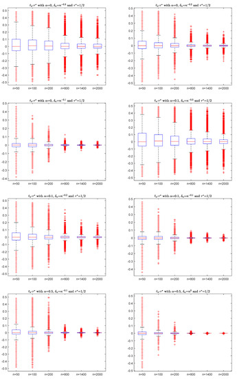
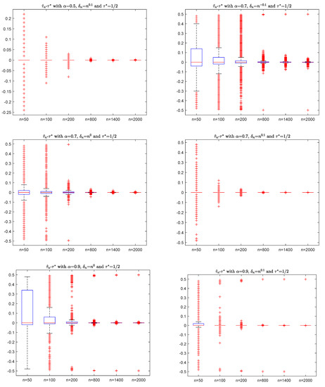
Figure 1. The box plots of ${\widehat{\tau }}_n\left(\alpha \right)-{\tau }^{*}$ with different $\alpha$ and ${\delta }_n$.

In Figure 1, the y-axis is the value of ${\widehat{\tau }}_n\left(\alpha \right)-{\tau }^{*}$, and the x-axis is the sample n. By the box plots in Figure 1, the differences of ${\widehat{\tau }}_n\left(\alpha \right)-{\tau }^{*}$ go to zero as sample n increases, which agrees with the consistency of (6) in Theorem 1. It has a similar performance if we take different values $\rho$, so the details are omitted here.

4. Real Data Examples

In this section, we use the CUSUM-type estimator ${\widehat{k}}_n\left(\alpha \right)=n{\widehat{\tau }}_n\left(\alpha \right)$ in (2) to do the mean change-point analysis with three real datasets. The first dataset is for the monthly mean temperature of Quebec in Canada from 1944 to 2008. The data can be found at http://climate.weather.gc.ca. For simplicity, we take the data of monthly mean temperatures for June and October, which contain 76 observations denoted by $x_{1,i}$ and $x_{2,i}$, $1\le i\le 76$, respectively. Let $x_i=x_{1,i}$ if $i=1,\dots ,76$ and $x_i=x_{2,i-76}$ if $i=76+1,\dots ,152$. Figure 2 shows the plot graph of $x_i$, $1\le i\le 152$, where the y-axis is the value of temperature $x_i$ and the x-axis is the sample n.

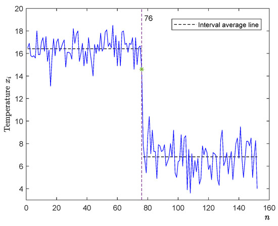
Figure 2. The plot graph of monthly mean temperatures based on June and October data.

Obviously, the mean temperature of June is different from that of October, so the change-point location $k^{*}$ is 76 (or ${\tau }^{*}=0.5$). Now, we use the CUSUM-type estimator ${\widehat{k}}_n\left(\alpha \right)$ to detect $k^{*}$, i.e., ${\widehat{k}}_n\left(\alpha \right)$ is defined by:

$${\widehat{k}}_n\left(\alpha \right)=\underset{1\le k\le n-1}{\mathrm{argmax}}\left|U_k\left(\alpha \right)\right|$$

(13)

where $0\le \alpha <1$ and:

$$U_k\left(\alpha \right)={\left(\frac{k(n-k)}{n}\right)}^{1-\alpha }\left(\frac{1}{k}\sum _{i=1}^k{x}_i-\frac{1}{n-k}\sum _{i=k+1}^n{x}_i\right),1\le k\le n-1.$$

Table 1 shows the values of ${\widehat{k}}_n\left(\alpha \right)$ with different values $\alpha$ such as $\alpha =0,0.1,\dots ,0.9$.

Table 1. The values of ${\widehat{k}}_n\left(\alpha \right)$ based on the temperature data.

$\mathit{\alpha }$	0	0.1	0.2	0.3	0.4	0.5	0.6	0.7	0.8	0.9
${\widehat{k}}_n\left(\alpha \right)$	76	76	76	76	76	76	76	76	76	76

By Table 1, the estimator ${\widehat{k}}_n\left(\alpha \right)$ with different $\alpha$ successfully detects the true change-point location $k^{*}=76$.

Second, we also use estimator ${\widehat{k}}_n\left(\alpha \right)$ to detect a time series of the annual flow of the Nile River at Aswan from 1871 to 1970 (see, for example, Zeileis et al. [26]). It measures annual discharge at Aswan in ${10}^8$ m³ and is depicted in Figure 3 (there are 100 observations denoted by $x_i$, $1\le i\le 100$). In Figure 3, the y-axis is the annual flow of the Nile River $x_i$, and the x-axis is the sample n.

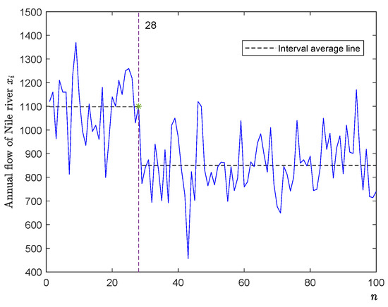
Figure 3. The plot graph of the annual flow of the Nile River from 1871 to 1970.

Similar to Table 1, the values of ${\widehat{k}}_n\left(\alpha \right)$ are given in Table 2.

Table 2. The values of ${\widehat{k}}_n\left(\alpha \right)$ based on the Nile River data.

$\mathit{\alpha }$	0	0.1	0.2	0.3	0.4	0.5	0.6	0.7	0.8	0.9
${\widehat{k}}_n\left(\alpha \right)$	28	28	28	28	28	28	28	28	28	28

By Table 2, we get a change-point location of 28 or equivalently the year 1898 (see Figure 3). On the other hand, Zeileis et al. [26] and Gao et al. [27] respectively used F-statistics and CUSUM statistics to detected the same change-point location of 28. It is well known that Aswan dam was built in 1898. It significantly changes the annual flow of the river Nile.

Lastly, we do the change-point analysis of returns based on a financial time series. Let $P_t$ be the closing prices of Tesla stock. Therefore, the return is defined as $r_t=log{P}_t-log{P}_{t-1}$. Figure 4 shows 138 daily returns on the prices of Tesla stock from 1 August 2016 to 13 February 2017. In Figure 4, the y-axis is the i-th return $r_i$, and the x-axis is the sample n. The data were downloaded from Yahoo Finance. Tesla announced on 22 November 2016 that it had completed the acquisition of SolarCity. It seams that the mean returns changed after that time of 22 November 2016 (the observation is 80). Therefore, we perform the test for this change-point of mean returns.

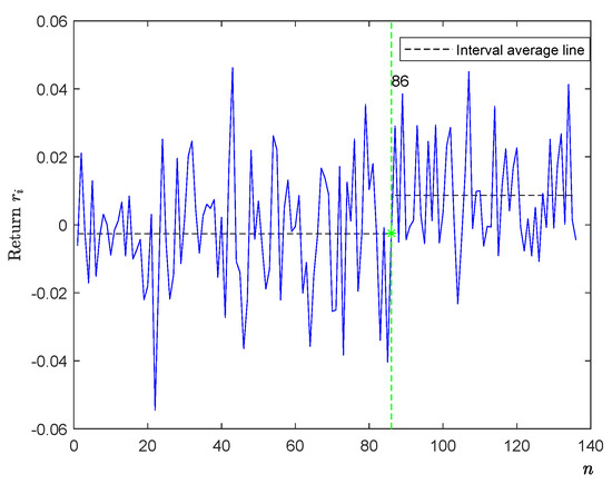
Figure 4. The plot graph of the mean returns of Tesla stock from 2016 to 2017.

Similar to Kokoszka and Leipus’s CUSUM estimator ${\widehat{k}}_n\left(\alpha \right)$ defined by (2), for any given $0\le \alpha <1$, Antoch et al. [17] investigated the following CUSUM estimator ${\tilde{k}}_n$ of $k^{*}$ defined as:

$${\tilde{k}}_n\left(\alpha \right)=\underset{1\le k\le n-1}{\mathrm{argmax}}\left|{\tilde{U}}_k\left(\alpha \right)\right|,$$

(14)

where:

$${\tilde{U}}_k\left(\alpha \right)={\left(\frac{n}{k(n-k)}\right)}^{\alpha }\sum _{i=1}^k\left(x_i-{\overline{x}}_n\right),1\le k\le n-1,$$

and ${\overline{x}}_n=\frac{1}{n}{\sum }_{i=1}^n{x}_i$. Therefore, we use these CUSUM-type estimators ${\widehat{k}}_n\left(\alpha \right)$ by (13) and ${\tilde{k}}_n\left(\alpha \right)$ by (14) to detect the change-point location $k^{*}$, where $x_i=r_i$, $1\le i\le 138$. With the different $\alpha =0,0.1,\dots ,0.9$, the values of ${\widehat{k}}_n\left(\alpha \right)$ and ${\tilde{k}}_n\left(\alpha \right)$ are presented in Table 3.

Table 3. The values of ${\widehat{k}}_n\left(\alpha \right)$ and ${\tilde{k}}_n\left(\alpha \right)$ based on Tesla’s returns data.

$\mathit{\alpha }$	0	0.1	0.2	0.3	0.4	0.5	0.6	0.7	0.8	0.9
${\widehat{k}}_n\left(\alpha \right)$	86	86	86	86	86	86	86	86	86	86
${\tilde{k}}_n\left(\alpha \right)$	86	86	86	86	86	86	86	86	86	86

By Table 3, the estimators ${\widehat{k}}_n\left(\alpha \right)$ and ${\tilde{k}}_n\left(\alpha \right)$ find the same change-point location of 86 (1 December 2016). Thus, the capital market recognized Tesla’s acquisition of SolarCity on 22 November of 2016, and the mean returns significantly changed from negative to positive after the time of 1 December 2016 (see Figure 4).

5. Conclusions

The CUSUM method is a popular method to detect the change-point. In this paper, we investigate the consistency of CUSUM-type estimator ${\widehat{\tau }}_n\left(\alpha \right)$ based on m-AANA sequences, which contain many dependent sequences such as NA, m-NA, and AANA sequences. Under the p-th moment ($1<p\le 2$) condition, we obtain a general consistency rate ${\widehat{\tau }}_n\left(\alpha \right)-{\tau }^{*}=O_P(g_n(\alpha ,p)/{\delta }_n)$, where $g_n(\alpha ,p)$ is defined by (6) and $0\le \alpha <1$. By taking ${\delta }_n={\delta }_0\ne 0$ in Theorem 1, we obtain the convergence rates as:

$${\widehat{\tau }}_n\left(\alpha \right)-{\tau }^{*}=\left\{\begin{array}{cc}{O}_P\left(n^{1/p-1}\right),\hfill & if0\le \alpha <\frac{1}{p},\hfill \\ O_P\left(n^{1/p-1}{log}^{1/p}n\right),\hfill & if\alpha =\frac{1}{p},\hfill \\ O_P\left(n^{\alpha -1}\right),\hfill & if\frac{1}{p}<\alpha <1.\hfill \end{array}\right.$$

Therefore, our Theorem 1 and Corollary 1 generalize the results of Kokoszka and Leipus [3]. In addition, ${\delta }_n$ in Theorem 1 can be taken as ${\delta }_n\to 0$ or ${\delta }_n\to \infty$, if $g_n(\alpha ,p)/{\delta }_n\to 0$ as $n\to \infty$. Let ${\delta }_n={\delta }_0\ne 0$ and $\left\{M\right(n),n\ge 1\}$ be any positive constant sequence satisfying $M\left(n\right)\to \infty$ and $M\left(n\right)/n=o\left(1\right)$. Shi et al. [16] obtained a strong convergence rate ${\widehat{\tau }}_n-{\tau }^{*}=o\left(\frac{M\left(n\right)}{n}\right)$, a.s. for the case of NA sequence. Our convergence rates are weaker than Shi et al. [16]; however, the m-AANA sequence is weaker than the NA sequence, and the change-amount ${\delta }_n$ can go to zero or infinity. In order to check our results, some simulations are shown in Figure 1, which agree with the consistency of Theorem 1. Lastly, three real dataset of Quebec temperature, Nile flow, and returns for Tesla in Section 4 are discussed to show that the CUSUM-type estimator ${\widehat{k}}_n\left(\alpha \right)$ defined by (13) can successfully detect the change-point location. In addition, it is interesting for scholars to study the strong convergence rate and limit distribution of CUSUM-type estimator ${\widehat{\tau }}_n\left(\alpha \right)$ based on the m-AANA sequence or other dependent sequences in future research. Furthermore, Shiryaev [25] discussed the stochastic disorder problems, which are known as the quickest detection problems. For example, Shiryaev [25] considered the Black–Scholes models with mean drift. Thus, we should pay attention to the applications of change-point models in mathematical finance and econometrics.

6. Proofs of the Main Results

For convenience, in the proofs, let $C,C_1,C_2,\dots$ be some positive constants that are independent of n and may have different values in different expressions.

Lemma 1.

(Theorem 3 of Nam et al. [7]). For some $1<p\le 2$, let $\{Z_n,n\ge 1\}$ be an m-AANA sequence of zero mean random variables with mixing coefficients $\left\{q\right(n),n\ge 1\}$ satisfying ${\sum }_{n=1}^{\infty }{q}^2\left(n\right)<\infty$. Let $\{b_n,n\ge 1\}$ be a nondecreasing sequence of positive numbers. Then, for any $\epsilon >0$ and any integer $n\ge 1$, we have:

$$P\left(\underset{1\le k\le n}{max}\left|\frac{1}{b_k}\sum _{j=1}^k{Z}_j\right|\ge \epsilon \right)\le \frac{2^p{m}^{p-1}{C}_p}{{\epsilon }^p}\sum _{j=1}^n\frac{E|Z_j{|}^p}{b_j^p},$$

where $C_p$ is a positive constant depending only on p.

Proof of Theorem 1.

Let ${\tau }_n=\lfloor k/n\rfloor$. For any given $0\le \alpha <1$, we have by (1) and (3) that:

$$\begin{array}{ccc}\hfill E{U}_k\left(\alpha \right)& =& {\left(\frac{k(n-k)}{n}\right)}^{1-\alpha }\left(\frac{1}{k}\sum _{i=1}^{k}E{X}_i-\frac{1}{n-k}\sum _{i=k+1}^{n}E{X}_i\right)\hfill \\ & =& \left\{\begin{array}{cc}-{\delta }_n{n}^{1-\alpha }{\tau }_n^{1-\alpha }{(1-{\tau }_n)}^{-\alpha }(1-{\tau }^{*}),\hfill & ifk\le k^{*},\hfill \\ -{\delta }_n{n}^{1-\alpha }{(1-{\tau }_n)}^{1-\alpha }{\tau }_n^{-\alpha }{\tau }^{*},\hfill & ifk>k^{*},\hfill \end{array}\right.\hfill \end{array}$$

(15)

and:

$$\begin{array}{c}\hfill E{U}_{k^{*}}\left(\alpha \right)=-{\delta }_n{n}^{1-\alpha }{\left({\tau }^{*}\right)}^{1-\alpha }{(1-{\tau }^{*})}^{1-\alpha }.\end{array}$$

(16)

Therefore, we have by (3.11) of Kokoszka and Leipus [3] that:

$$|{\delta }_n|\overline{\tau }{n}^{1-\alpha }|{\widehat{\tau }}_n-{\tau }^{*}|\le 2\underset{1\le k\le n-1}{max}|U_k\left(\alpha \right)-E{U}_k\left(\alpha \right)|,$$

(17)

where $\overline{\tau }:=(1-\alpha ){\left({\tau }^{*}\right)}^{-\alpha }{(1-{\tau }^{*})}^{-\alpha }min\{{\tau }^{*},1-{\tau }^{*}\}$. By (1) and (3), it is easy to see that:

$$\begin{array}{ccc}\hfill n^{\alpha -1}\underset{1\le k\le n-1}{max}|U_k\left(\alpha \right)-E{U}_k\left(\alpha \right)|& \le & n^{\alpha -1}\underset{1\le k\le n-1}{max}\frac{1}{k^{\alpha }}\left|\sum _{i=1}^k(X_i-E{X}_i)\right|\hfill \\ & & +n^{\alpha -1}\underset{1\le k\le n-1}{max}\frac{1}{{(n-k)}^{\alpha }}\left|\sum _{i=k+1}^n(X_i-E{X}_i)\right|\hfill \\ & =& n^{\alpha -1}\underset{1\le k\le n-1}{max}\frac{1}{k^{\alpha }}\left|\sum _{i=1}^k{Z}_i\right|+n^{\alpha -1}\underset{1\le k\le n-1}{max}\frac{1}{{(n-k)}^{\alpha }}\left|\sum _{i=k+1}^n{Z}_i\right|\hfill \\ & :=& D_1+D_2.\hfill \end{array}$$

(18)

By (5), (17), and (18), in order to prove (6), we have to prove that:

$$D_i=O_P\left(g_n(\alpha ,p)\right),i=1,2,$$

(19)

where $g_n(\alpha ,p)$ is defined (5). On the one hand, for any $\epsilon >0$, it follows from Lemma 1 with $\underset{n\ge 1}{sup}E{\left|Z_n\right|}^p<\infty$ that:

$$\begin{array}{ccc}\hfill P\left(\underset{1\le k\le n-1}{max}\frac{1}{k^{\alpha }}\left|\sum _{i=1}^k{Z}_i\right|>\epsilon n^{1-\alpha }\right)& \le & \frac{C_1}{{\left(\epsilon n^{1-\alpha }\right)}^p}\sum _{i=1}^n\frac{E|Z_i{|}^p}{i^{\alpha p}}\hfill \\ & \le & \frac{C_2}{{\epsilon }^p{n}^{p-\alpha p}}\sum _{i=1}^n\frac{E|Z_i{|}^p}{i^{\alpha p}}\hfill \\ & \le & \left\{\begin{array}{cc}{C}_3{\epsilon }^{-p}{n}^{1-p}\hfill & if0\le \alpha <\frac{1}{p},\hfill \\ C_4{\epsilon }^{-p}{n}^{1-p}logn\hfill & if\alpha =\frac{1}{p},\hfill \\ C_5{\epsilon }^{-p}{n}^{p(\alpha -1)}\hfill & if\frac{1}{p}<\alpha <1,\hfill \end{array}\right.\hfill \end{array}$$

(20)

where $C_i$, $i=1,\dots ,5$, are positive constants independentof n. Consequently, by (18)–(20), we have:

$$D_1=O_P\left(g_n(\alpha ,p)\right).$$

On the other hand, it can be checked that:

$$D_2=n^{\alpha -1}\underset{1\le k\le n-1}{max}\frac{1}{{(n-k)}^{\alpha }}\left|\sum _{i=k+1}^n{Z}_i\right|=n^{\alpha -1}\underset{1\le k<n}{max}\frac{1}{k^{\alpha }}\left|\sum _{i=1}^k{Z}_{n-i+1}\right|.$$

Therefore, one can obtain analogously the same result that

$$D_2=O_P\left(g_n(\alpha ,p)\right).$$

Thus, the proof of (6) is completed.  □

Proof of Corollary 1.

By taking ${\delta }_n={\delta }_0\ne 0$ in Theorem 1, one can immediately obtain Corollary 1.  □

References

- Csörgő, M.; Horváth, L. Limit Theorems in Change-Point Analysis; Wiley: Chichester, UK, 1997; pp. 170–181. [Google Scholar]
- Shiryaev, A. On stochastic models and optimal methods in the quickest detection problems. Theory Probab. Appl. 2009, 53, 385–401. [Google Scholar] [CrossRef]
- Kokoszka, P.; Leipus, R. Change-point in the mean of dependent observations. Stat. Probab. Lett. 1998, 40, 385–393. [Google Scholar] [CrossRef]
- Block, H.W.; Savits, T.H.; Shaked, M. Some concepts of negative dependence. Ann. Probab. 1982, 10, 765–772. [Google Scholar] [CrossRef]
- Chandra, T.K.; Ghosal, S. The strong law of large numbers for weighted averages under dependence assumptions. J. Theoret. Probab. 1996, 9, 797–809. [Google Scholar] [CrossRef]
- Hu, T.C.; Chiang, C.Y.; Taylor, R.L. On complete convergence for arrays of rowwise m-negatively associated random variables. Nonlinear Anal. 2009, 71, e1075–e1081. [Google Scholar] [CrossRef]
- Nam, T.; Hu, T.; Volodin, A. Maximal inequalities and strong law of large numbers for sequences of m-asymptotically almost negatively associated random variables. Commun. Stat. Theory Methods 2017, 46, 2696–2707. [Google Scholar] [CrossRef]
- Ko, M. Hájek-Rényi inequality for m-asymptotically almost negatively associated random vectors in Hilbert space and applications. J. Inequal. Appl. 2018, 2018, 80. [Google Scholar] [CrossRef]
- Bulinski, A.V.; Shaskin, A. Limit Theorems for Associated Random Fields and Related Systems; World Scientific: Singapore, 2007; pp. 1–20. [Google Scholar]
- Chen, P.; Hu, T.C.; Volodin, A. On complete convergence for arrays of row-wise negatively associated random variables. Theory Probab. Appl. 2008, 52, 323–328. [Google Scholar] [CrossRef]
- Yuan, D.M.; An, J. Rosenthal type inequalities for asymptotically almost negatively associated random variables and applications. Sci. China Ser. A 2009, 52, 1887–1904. [Google Scholar] [CrossRef]
- Chen, Z.Y.; Wang, X.J.; Hu, S.H. Strong laws of large numbers for weighted sums of asymptotically almost negatively associated random variables. Rev. Real Acad. Cienc. Exactas Fis. Nat. Ser. A Mat. 2015, 109, 135–152. [Google Scholar] [CrossRef]
- Wu, Y.F.; Hu, T.C.; Volodin, A. Complete convergence and complete moment convergence for weighted sums of m-NA random variables. J. Inequal. Appl. 2015, 2015, 200. [Google Scholar] [CrossRef]
- Xi, M.M.; Deng, X.; Wang, X.J.; Cheng, Z.Y. Lp convergence and complete convergence for weighted sums of AANA random variables. Commun. Stat. Theory Methods 2018, 47, 5604–5613. [Google Scholar] [CrossRef]
- Ye, R.Y.; Liu, X.S.; Yu, Y.C. Pointwise optimality of wavelet density estimation for negatively associated biased sample. Mathematics 2020, 8, 176. [Google Scholar] [CrossRef]
- Shi, X.; Wu, Y.; Miao, B. Strong convergence rate of estimators of change point and its application. Comput. Stat. Data Anal. 2009, 53, 990–998. [Google Scholar] [CrossRef]
- Antoch, J.; Hušková, M.; Veraverbeke, N. Change-point problem and bootstrap. J. Nonparametr. Stat. 1995, 5, 123–144. [Google Scholar] [CrossRef]
- Lee, S.; Ha, J.; Na, O. The cusum test for parameter change in time series models. Scand. J. Stat. 2003, 30, 781–796. [Google Scholar] [CrossRef]
- Chen, J.; Gupta, A. Parametric Sstatistical Change Point Analysiswith Applications to Genetics Medicine and Finance, 2nd ed.; Birkhäuser: Boston, MA, USA, 2012; pp. 1–30. [Google Scholar]
- Horváth, L.; Hušková, M. Change-point detection in panel data. J. Time Ser. Anal. 2012, 33, 631–648. [Google Scholar] [CrossRef]
- Horváth, L.; Rice, G. Extensions of some classical methods in change point analysis. Test 2014, 23, 219–255. [Google Scholar] [CrossRef]
- Messer, M.; Albert, S.; Schneider, G. The multiple filter test for change point detection in time series. Metrika 2018, 81, 589–607. [Google Scholar] [CrossRef]
- Xu, M.; Wu, Y.; Jin, B. Detection of a change-point in variance by a weighted sum of powers of variances test. J. Appl. Stat. 2019, 46, 664–679. [Google Scholar] [CrossRef]
- Abbas, N.; Abujiya, M.A.R.; Riaz, M.; Mahmood, T. Cumulative sum chart modeled under the presence of outliers. Mathematics 2020, 8, 269. [Google Scholar] [CrossRef]
- Shiryaev, A. Stochastic Disorder Problems; Springer: Berlin/Heidelberg, Germany, 2019; pp. 367–388. [Google Scholar]
- Zeileis, Z.; Kleiber, C.; Krämer, W.; Hornik, K. Testing and dating of structural changes in practice. Comput. Stat. Data Anal. 2003, 44, 109–123. [Google Scholar] [CrossRef]
- Gao, M.; Ding, S.S.; Wu, S.P.; Yang, W.Z. The asymptotic distribution of CUSUM estimator based on α-mixing sequences. Commun. Stat.-Simul. Comput. 2020. [Google Scholar] [CrossRef]
Publisher’s Note: MDPI stays neutral with regard to jurisdictional claims in published maps and institutional affiliations. |
© 2020 by the authors. Licensee MDPI, Basel, Switzerland. This article is an open access article distributed under the terms and conditions of the Creative Commons Attribution (CC BY) license (http://creativecommons.org/licenses/by/4.0/).