Fixed Point Sets of Digital Curves and Digital Surfaces

Abstract

Given a digital image (or digital object) $(X,k)$, we address some unsolved problems related to the study of fixed point sets of k-continuous self-maps of $(X,k)$ from the viewpoints of digital curve and digital surface theory. Consider two simple closed k-curves with $l_i$ elements in ${\mathbb{Z}}^n$, $i\in \{1,2\},l_1⪈l_2\ge 4$. After initially formulating an alignment of fixed point sets of a digital wedge of these curves, we prove that perfectness of it depends on the numbers $l_i,i\in \{1,2\}$, instead of the k-adjacency. Furthermore, given digital k-surfaces, we also study an alignment of fixed point sets of digital k-surfaces and digital wedges of them. Finally, given a digital image which is not perfect, we explore a certain condition that makes it perfect. In this paper, each digital image $(X,k)$ is assumed to be k-connected and $X^{♯}\ge 2$ unless stated otherwise.

1. Introduction

Throughout this paper, we denote by $\mathbb{Z}$ (resp.$\mathbb{N}$) the set of integers (resp. natural numbers), and let ${\mathbb{Z}}^n$ be the n times Cartesian product of $\mathbb{Z}$, $n\in \mathbb{N}$. Besides, let ${\mathbb{N}}_1$ (resp.${\mathbb{N}}_0$) be the set of odd (resp. even) natural numbers. Motivated by the study of fixed point sets in [1], we are currently interested in the set of fixed point sets of a digital image $(X,k)$ [2,3,4] because it can be applied in the fields of applied sciences and robotics [5].

Given a digital image (or digital object) $(X,k)$, the authors of [2] explored some features of fixed point sets of k-continuous self-maps of it. The works in [3,4] further studied this topic to obtain many results. However, there are still many unsolved problems related to this work. To be precise, given a digital image $(X,k)$, let $Co{n}_k(X)$ be the set $\{f | f \mathrm{is} \mathrm{a} k-\mathrm{continuous} \mathrm{map} \mathrm{of} (X,k)\}$. Besides, let us recall that [2,4]

$$F(Co{n}_k(X)):=\{Fix{(f)}^{♯} | f\in Co{n}_k(X)\}$$

where $Fix(f):=\{x\in X | f(x)=x\},$ $‘‘:=$” is used for introducing a new terminology or a notation. We denote by $F(Co{n}_k(X)))$ an alignment of fixed point sets of $(X,k)$ (for more details see Definition 2).

Given a simple closed k-curve with l elements in ${\mathbb{Z}}^n$, denoted by $C_k^{n,l}$, it turns out that $F(Co{n}_k(C_k^{n,l}))$ is perfect if and only if $C_k^{n,l}$ is k-contractible, i.e., $l=4$ [3,4]. Besides, only for the case $l(\ge 4)\in {\mathbb{N}}_0$ or $l(\ge 7)\in {\mathbb{N}}_1$, the study of $F(Co{n}_k(C_k^{n,l}\vee C_k^{n,l}))$ was recently done [4]. However, in the cases $l_1\in {\mathbb{N}}_1$ and $l_2\in {\mathbb{N}}_0$, and $l_1,l_2(\ge 5)\in {\mathbb{N}}_1$, the study of $F(Co{n}_k(C_k^{n,l_1}\vee C_k^{n,l_2}))$ remains open, as follows.

(Q1) Given two simple closed k-curves $C_k^{n,l_1}$ and $C_k^{n,l_2}$, where $l_1\in {\mathbb{N}}_1\backslash \{1,3\}$ and $l_2\in {\mathbb{N}}_0\backslash \left\{2\right\}$, how can we formulate $F(Co{n}_k(C_k^{n,l_1}\vee C_k^{n,l_2}))$?

(Q2) Unlike the hypothesis of (Q1), given $l_1,l_2(\ge 5)\in {\mathbb{N}}_1$, how can we formulate $F(Co{n}_k(C_k^{n,l_1}\vee C_k^{n,l_2}))$?

With the hypothesis of $‘‘$$l_1\in {\mathbb{N}}_1$, $l_2\in {\mathbb{N}}_0$, or $l_1,l_2(\ge 5)\in {\mathbb{N}}_1$”, the following queries are raised.

(Q3) How many 2-components are there in $F(Co{n}_k(C_k^{n,l_1}\vee C_k^{n,l_2}))$ ?

(Q4) Are there some relationships among the numbers $l_1,l_2$, and the perfectness of $F(Co{n}_k(C_k^{n,l_1}\vee C_k^{n,l_2}))$ ?

(Q5) Given a simple k-path $(P,k)$ with d as the length of it, what conditions make $F(Co{n}_k(C_k^{n,l_1}\vee C_k^{n,l_2}\vee P))$ perfect ?

(Q6) How can we characterize $F(Co{n}_k(C_k^{n,l_1}\vee C_k^{n,l_2}\vee \stackrel{\mathrm{t}-\mathrm{times}}{\overbrace{C_k^{n,4}\vee \cdots \vee C_k^{n,4}}}))$ ?

After addressing these queries, we will adapt these kinds of approaches into the study of fixed point sets of some digital k-surfaces in ${\mathbb{Z}}^3$ [6,7,8,9,10,11,12]. Let $(S_i,k)$ be a digital k-surface in ${\mathbb{Z}}^3,i\in \{1,2\}$, and $(S_1\vee S_2,k)$ be a digital wedge of $(S_i,k),i\in \{1,2\}$. In particular, we denote a minimal simple closed 18-surface consisting of ten (resp. six) elements in ${\mathbb{Z}}^3$ by $MS{S}_{18}$ (resp. $MS{S}_{18}^{\prime }$) [10,11] (see also Section 6). Then, the following issues are naturally raised.

(Q7) Given a digital k-surface $S_k$, how can we formulate $F(Co{n}_k(S_k))$ and $F(Co{n}_k(S_k\vee MS{S}_{18}^{\prime }))$ ?

(Q8) For a digital k-surface $S_k$, how many 2-components are there in $F(Co{n}_k(S_k))$ ?

(Q9) Under what conditions are $F(Co{n}_k(S_k))$, $F(Co{n}_{18}(MS{S}_{18}))$, and $F(Co{n}_{18}(MS{S}_{18}\vee MS{S}_{18}))$ perfect ?

Using many new tools, we shall address all of these issues.

The remaining part of the paper is organized as follows. Section 2 recalls some notions and backgrounds needed for this study. Besides, it refers to some properties of digital continuity. Section 3 initially formulates $F(Co{n}_k(C_k^{n,l}\vee C_k^{n,4}))$ with a certain hypothesis, where $l(\ge 5)\in {\mathbb{N}}_1$, and explores a certain condition which makes it perfect. Section 4 investigates the number of the 2-components of $F(Co{n}_k(C_k^{n,l_1}\vee C_k^{n,l_2}))$, where $l_1(\ge 5)\in {\mathbb{N}}_1,l_2(\ge 6)\in {\mathbb{N}}_0,k\ne 2n$. Besides, after joining a simple k-path $(P,k)$ onto $C_k^{n,l_1}\vee C_k^{n,l_2}$ to produce a digital wedge $(C_k^{n,l_1}\vee C_k^{n,l_2}\vee P,k)$, we investigate a certain condition that makes $F(Co{n}_k(C_k^{n,l_1}\vee C_k^{n,l_2}\vee P))$ perfect. Finally, we investigate certain conditions that make $F(Co{n}_k(C_k^{n,l_1}\vee C_k^{n,l_2}\vee \stackrel{\mathrm{t}-\mathrm{times}}{\overbrace{C_k^{n,4}\vee \cdots \vee C_k^{n,4}}}))$ perfect. Section 5 investigate some properties of $F(Co{n}_k(C_k^{n,l_1}\vee C_k^{n,l_2}))$, where $l_1,l_2(\ge 7)\in {\mathbb{N}}_1,k\ne 2n$. In addition, we also deal with $F(Co{n}_k(C_k^{n,l}\vee C_k^{n,5}))$ with a certain hypothesis (see the property (4)). Section 6 develops several types of fixed point theorems for digital k-surfaces. Namely, for some digital k-surfaces $(S_i,k),i\in \{1,2\}$ and $(S_1\vee S_2,k)$, we formulate $F(Co{n}_k(S_i))$ and $F(Co{n}_k(S_1\vee S_2))$ and investigate some properties of them. Eventually, we shall address the issues (Q7)-(Q9). Section 7 concludes the paper. In addition, we will denote the cardinality of a set X with $X^{♯}$.

2. Digital Wedges and Some Properties of the Digital Continuity

As an initial version of a digital image, a pair $(X,k)$ was called a digital image, where $X\subset {\mathbb{Z}}^n$ and the k-adjacency of ${\mathbb{Z}}^n$ was assumed in $n\in \{1,2,3\}$ [13,14,15]. After then, the work in [16] first generalized this approach into the high-dimensional digital image $X\subset {\mathbb{Z}}^n$ with one of the k-adjacency relations of ${\mathbb{Z}}^n,n\in \mathbb{N}$. To study $X\subset {\mathbb{Z}}^n$ in a digital topological setting, $n\in \mathbb{N}$, the following digital k-adjacency (or digital k-connectivity) was taken in [16] (see also in [17]), as follows.

For a natural number t, $1\le t\le n$, the two distinct points

$$p=(p_1,p_2,\cdots ,p_n) \mathrm{and} q=(q_1,q_2,\cdots ,q_n)\in {\mathbb{Z}}^n,$$

are $k(t,n)$-adjacent if at most t of their coordinates differ by $\pm 1$ and the others coincide. According to this statement, the $k(t,n)$-adjacency relations of ${\mathbb{Z}}^n,n\in \mathbb{N}$, are formulated [16] (see also in [17]) as follows,

$$k:=k(t,n)=\sum _{i=1}^t{2}^i{C}_i^n,\mathrm{where} C_i^n:=\frac{n!}{(n-i)!i!}.$$

(1)

For instance [16,17],

$$(n,t,k)\in \left\{\begin{array}{l}(3,1,6),(3,2,18),(3,3,26);\\ (4,1,8),(4,2,32),(4,3,64),(4,4,80);\mathrm{and}\\ (5,1,10),(5,2,50),(5,3,130),(5,4,210),(5,5,242).\end{array}\right.$$

Hereafter, $(X,k)$ is assumed in ${\mathbb{Z}}^n,n\in \mathbb{N}$, with one of the k-adjacency of (1). Besides, these k-adjacency relations are strongly used in calculating digital k-fundamental groups of digital products [16,18]. Indeed, a digital image $(X,k)$ is one of digital spaces [19] (see also in [11]). For $x,y\in \mathbb{Z}$ with $x⪇y$, the set ${[x,y]}_{\mathbb{Z}}=\{n\in \mathbb{Z} | x\le n\le y\}$ with 2-adjacency is called a digital interval [13,20].

The following terminology and notions [11,13,14,15,16,20,21] will be also used later. Given $(X,k)$ with $X^{♯}\ge 2$, by a k-path with $l+1$ elements in X we mean the sequence ${(x_i)}_{i\in {[0,l]}_{\mathbb{Z}}}\subset X$ such that $x_i$ and $x_j$ are k-adjacent if $| i-j |=1$ [13]. We say that $(X,k)$ is k-connected if for any distinct points $x,y\in X$ there is a k-path ${(x_i)}_{i\in {[0,l]}_{\mathbb{Z}}}$ in X such that $x_0=x$ and $x_l=y$ [13,20] (for more details see in [11]). Given $(X,k)$, by the k-component of $x\in X$, we mean the maximal k-connected subset of $(X,k)$ containing the point x [13].

By a simple k-path from x to y in $(X,k)$, we mean a finite set ${(x_i)}_{i\in {[0,m]}_{\mathbb{Z}}}\subset {\mathbb{Z}}^n$ such that $x_i$ and $x_j$ are k-adjacent if and only if $| i-j |=1$, where $x_0=x$ and $x_m=y$ [13]. Then, the length of this set ${(x_i)}_{i\in {[0,m]}_{\mathbb{Z}}}$ is denoted by $l_k(x,y):=m$.

By a simple closed k-curve (or simple k-cycle) with l elements in ${\mathbb{Z}}^n,n\ge 2$, denoted by $S{C}_k^{n,l}$ [13,16], $l\ge 4$, we mean a set ${(x_i)}_{i\in {[0,l-1]}_{\mathbb{Z}}}\subset {\mathbb{Z}}^n$ such that $x_i$ and $x_j$ are k-adjacent if and only if $| i-j |=\pm 1 (mod l)$. Then, the number l of $S{C}_k^{n,l}$ depends on both the dimension n of ${\mathbb{Z}}^n$ and the k-adjacency (for details, see the property (2) below). Hereafter, we use the notation $C_k^{n,l}$ to abbreviate $S{C}_k^{n,l}$.

As to the number l of $C_k^{n,l},n\in \mathbb{N}\backslash \left\{1\right\},l\ge 4$, according to the k-adjacency of ${\mathbb{Z}}^n$ in (1), some properties of the number l of $C_k^{n,l}$, are obtained, as follows [4].

$$\left\{\begin{array}{l}(1) \mathrm{in} \mathrm{the} \mathrm{case} k=2n(n\ne 2), \mathrm{we} \mathrm{have} l \in {\mathbb{N}}_0\backslash \left\{2\right\};\\ (2) \mathrm{in} \mathrm{the} \mathrm{case} k=4, \mathrm{we} \mathrm{obtain} l \in {\mathbb{N}}_0\backslash \{2,6\},i.e., \mathrm{neither} C_4^{2,5} \mathrm{nor} C_4^{2,6} \mathrm{exists};\\ (3) \mathrm{in} \mathrm{the} \mathrm{case} k=8, \mathrm{we} \mathrm{have} l \in \mathbb{N}\backslash \{1,2,3,5\}. \mathrm{Naively}, \mathrm{no} C_8^{2,5} \mathrm{exists};\\ (4) \mathrm{in} \mathrm{the} \mathrm{case} k=18, \mathrm{we} \mathrm{obtain} l \in \mathbb{N}\backslash \{1,2,3,5\}; \mathrm{and}\\ (5) \mathrm{in} \mathrm{the} \mathrm{case} k:=k(t,n),3\le t\le n, \mathrm{we} \mathrm{have} l \in \mathbb{N}\backslash \{1,2,3\}.\\ \mathrm{Namely}, \mathrm{neither} C_6^{2,5} \mathrm{nor} C_{18}^{3,5} \mathrm{exists}. \mathrm{However}, C_{26}^{3,5} \mathrm{exists}.\end{array}\right.$$

(2)

This is an improved version of (2) in [4] because there is a misprint at the fourth line of (2) in [4]. For the cases of (3)–(4) of (2), $C_8^{2,7}$ and $C_{18}^{3,9}$ are considered (see Figure 1). Hereafter, in terms of the number l of $C_k^{n,l}$, we will follow the property (2).

As the notion of neighborhood plays an important role in digital topology and digital geometry, a digital k-neighborhood of a point p of a digital image $(X,k)$ was established, as follows. Given $(X,k)$ and a point $p\in X$, the following notion of ‘digital k-neighborhood of p with radius 1’ is defined, as follows [16].

$$N_k(p,1):=\{x\in X | x \mathrm{is} k-\mathrm{adjacent} \mathrm{to} p\}\cup \left\{p\right\}.$$

(3)

By using the notion of (3), the digital $(k_0,k_1)$-continuity of a map $f:(X,k_0)\to (Y,k_1)$ in [15] was represented, as follows [10,16].

Proposition 1

([10,16]). A function $f:(X,k_0)\to (Y,k_1)$ is (digitally) $(k_0,k_1)$-continuous if and only if for every $x\in X$, $f(N_{k_0}(x,1))\subset N_{k_1}(f(x),1)$.

In Proposition 1, in the case $k:=k_0=k_1$, the map f is called a “k-continuous” map to abbreviate the $(k,k)$-continuity of the given map f. In some literature, as there is some confusion of the digital k-continuity of a map between digital images, we need to attention the following.

Theorem 1.

Given a set $X\subset {\mathbb{Z}}^n$, let us consider the two digital connectivities of X such as $k(t_1,n)$ and $k(t_2,n)$ with $t_1⪇t_2$ (see the property of (1)). Naively, assume the two digital images $(X,k(t_1,n))$ and $(X,k(t_2,n))$. Further consider a $k(t_1,n)$-continuous self-map of $(X,k(t_1,n))$ and a $k(t_2,n)$-continuous self-map of $(X,k(t_2,n))$. Then, neither of them implies the other.

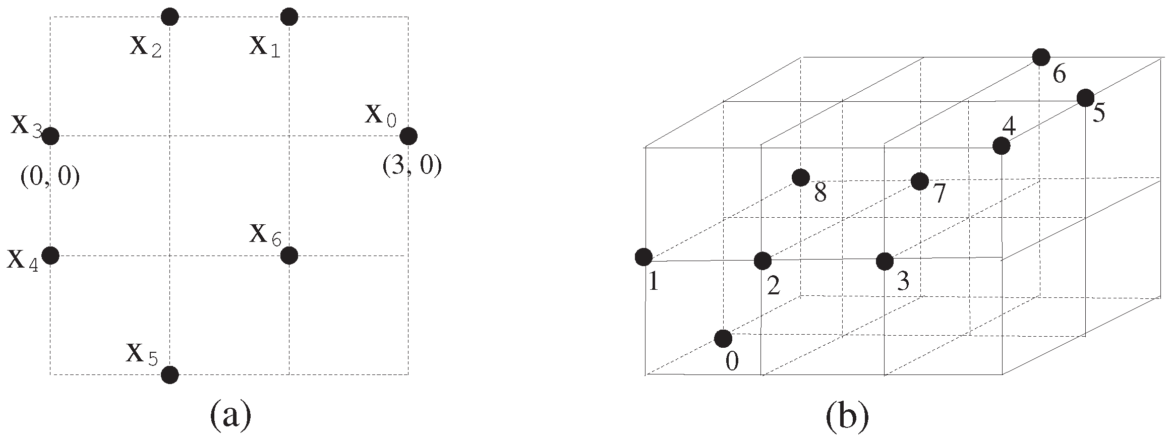
Proof. 

Using Proposition 1, we prove the assertion. First, we prove that the $k_2$-continuity of a self-map of $(X,k_2:=k(t_2,n))$ need not imply the $k_1$-continuity of a self-map of $(X,k_1:=k(t_1,n)),t_1⪇t_2$ with the following counterexample. Let us consider the self-map of $(X_1:=\{a,b,c\},26)$ such as $f_1:(X_1,26)\to (X_1,26)$ (see Figure 2a) such that $f_1(a)=a,f_1(\{b,c\})=\left\{c\right\}$. While the map $f_1$ is obviously a 26-continuous map, it is neither 18- nor 6-continuous at the point $a\in X_1$ because

$$\left\{\begin{array}{l}{f}_1(N_{18}(a,1))=\{a,c\}⊈N_{18}(f(a),1))=\{a,b\} \mathrm{and}\\ f_1(N_6(a,1))=\{a,c\}⊈N_6(f(a),1))=\{a,b\},\end{array}\right.$$

where $N_{18}(a,1)=\{a,b\}=N_6(a,1)$.

Similarly, taking a certain example similar to the map $f_1$ above, we can clearly prove that for a certain digital image $(Y,18)$ an 18-continuous map need not imply a 6-continuous map at a certain point $y\in Y$.

Conversely, we prove that the $k_1$-continuity of a self-map of $(X,k_1:=k(t_1,n))$ need not imply the $k_2$-continuity of a self-map of $(X,k_2:=k(t_2,n))$ with the following counterexample. Let us consider the self-map of $(X_2:=\{a,b,c,d\},6)$ such as $f_2:(X_2,6)\to (X_2,6)$ (see Figure 2b) such that

$$f_2(a)=b,f_2(b)=c,f_2(\{c,d\})=\left\{d\right\}.$$

While the map $f_2$ is a 6-continuous map, it is neither 18- nor 26-continuous at the point $a\in X_2$ because

$$f_2(N_{18}(a,1))=f_2(\{a,b,c\})=\{b,c,d\}⊈N_{18}(f_2(a),1))=\{a,b,c\},$$

and similarly we obtain

$$f_2(N_{26}(a,1))=\{b,c,d\}⊈N_{26}(f_2(a),1))=\{a,b,c\},$$

where $N_{18}(a,1)=\{a,b,c\}=N_{26}(a,1)$.

As another example, let us consider the self-map of $(X_3:=\{a,b,c,d\},18)$ such as $f_3:(X_3,18)\to (X_3,18)$ (see Figure 2c) such that

$$f_3(a)=b,f_3(b)=c,f_3(\{c,d\})=\left\{d\right\}.$$

While the map $f_3$ is an 18-continuous map, it is not 26-continuous at the point $a\in X_3$ because

$$f_3(N_{26}(a,1))=f_3(\{a,b,c\})=\{b,c,d\}⊈N_{26}(f_3(a),1))=\{a,b,c\},$$

where $N_{26}(a,1)=\{a,b,c\}$. □

In view of Theorem 1, we observe that not every $k_1$-continuous self-map of $(X,k_1)$ implies a $k_2$-continuous self-map of $(X,k_2)$ if $k_1\ne k_2$. Namely, we observe that a $k_1$-continuous self-map of $(X,k_1)$ is different from a $k_2$-continuous self-map of $(X,k_2)$ if $k_1\ne k_2$.

Using the digital continuity of maps between two digital images, let us recall the category DTC consisting of the following two pieces of data [16], called the “digital topological category”, as follows.

• The set of $(X,k)$, where $X\subset {\mathbb{Z}}^n$, as objects of DTC denoted by $Ob(DTC)$;
• For every ordered pair of objects $(X_i,k_i),i\in \{0,1\}$, the set of all $(k_0,k_1)$-continuous maps between them as morphisms of DTC, denoted by $Mor(DTC)$.
  In DTC, for the case $k:=k_0=k_1$, we will use the notation DTC(k) [18].

To compare digital images $(X,k)$ [22] up to similarity, we often use the notion of $(k_0,k_1)$-isomorphism (or k-isomorphism) as in [22]), as follows.

Definition 1

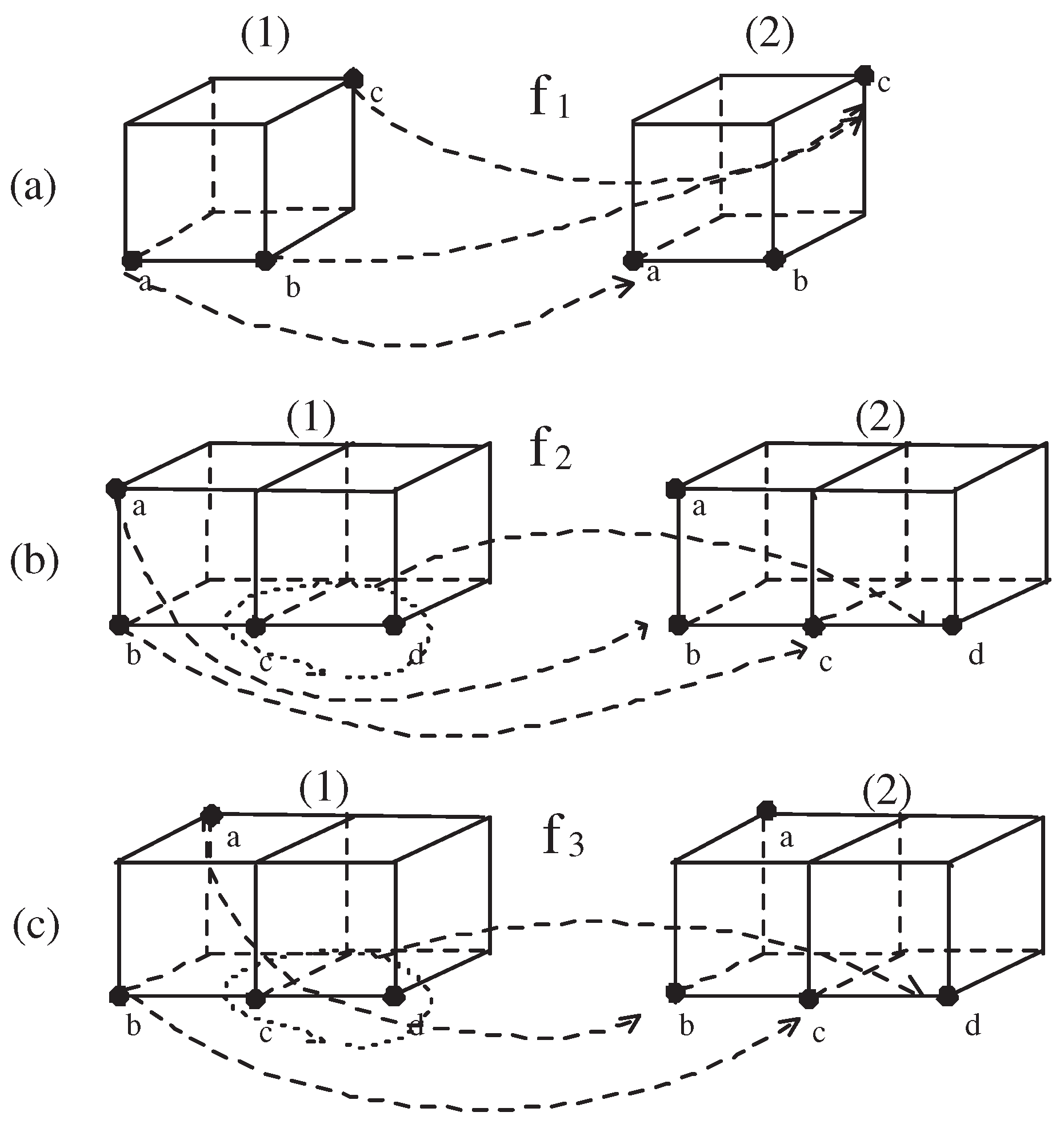
([22]). ($(k_0,k_1)$-homeomorphism in [23]) Consider two digital images $(Z,k_0)$ and $(W,k_1)$ in ${\mathbb{Z}}^{n_0}$ and ${\mathbb{Z}}^{n_1}$, respectively. Then, a map $h:Z\to W$ is called a $(k_0,k_1)$-isomorphism if h is a $(k_0,k_1)$-continuous bijection and further, $h^{-1}:W\to Z$ is $(k_1,k_0)$-continuous. Then, we use the notation $Z{\approx }_{(k_0,k_1)}W$. In the case $k:=k_0=k_1$, the map h is called a k-isomorphism.

Let us now recall the notions of a digital wedge which can be used in studying fixed point sets from the viewpoint of digital geometry. Given two digital images $(A,k)$ and $(B,k)$, a digital wedge of them, denoted by $(A\vee B,k)$, is initially defined [16,18] as the union of the digital images $(A^{\prime },k)$ and $(B^{\prime },k)$ (for more details see Figure 3a), where

(1)

$A^{\prime }\cap B^{\prime }$ is a singleton, say $\left\{p\right\}$;

(2)

$A^{\prime }\backslash \left\{p\right\}$ and $B^{\prime }\backslash \left\{p\right\}$ are not k-adjacent, where two sets $(C,k)$ and $(D,k)$ are said to be k-adjacent if $C\cap D=\varnothing$ and there are at least two points $a\in C$ and $b\in D$ such that a is k-adjacent to b [20]; and

(3)

$(A^{\prime },k)$ is k-isomorphic to $(A,k)$ and $(B^{\prime },k)$ is k-isomorphic to $(B,k)$ (see Definition 1).

In view of this feature, we may consider $(A\vee B,k)$ to be $(A^{\prime }\vee B^{\prime },k)$. When studying digital wedges in a digital topological setting, we are strongly required to follow this approach. Indeed, this digital wedge is quite different from the classical one point union (or wedge) in typical topology [24] and standard graph theory [25] by the k-adjacency referred to in (2) above. Based on the property (2), given $C_k^{n,l_1}\vee C_k^{n,l_2}$ such that $l_1\in {\mathbb{N}}_1$ and $l_2\in {\mathbb{N}}_0$, we observe the following properties.

$$\left\{\begin{array}{l}(1) k\ne 2n; \mathrm{and}\\ (2) l_1(\ge 7)\in {\mathbb{N}}_1,l_2\in {\mathbb{N}}_0\backslash \left\{2\right\} \mathrm{if} k=8, n=2;\\ (3) l_1(\ge 7)\in {\mathbb{N}}_1,l_2\in {\mathbb{N}}_0\backslash \left\{2\right\} \mathrm{if} k=18, n=3; \mathrm{and}\\ (4) l_1(\ge 5)\in {\mathbb{N}}_1,l_2\in {\mathbb{N}}_0\backslash \left\{2\right\} \mathrm{if} k:=k(t,n),3\le t\le n.\end{array}\right\}$$

(4)

In the case $n\ge 4$, depending on the numbers t and n of $k:=k(t,n)$, we can take $l_1\ge 5$ or $l_1\ge 7$. Hereafter, as to $l_i,i\in \{1,2\}$, of $C_k^{n,l_1}\vee C_k^{n,l_2}$, we will follow the property of (4). In relation to (4), we may similarly consider the cases $l_1\in {\mathbb{N}}_0$ and $l_2\in {\mathbb{N}}_1$ because $(C_k^{n,l_1}\vee C_k^{n,l_2},k)$ is k-isomorphic to $(C_k^{n,l_2}\vee C_k^{n,l_1},k)$.

3. Formulation of $\mathit{F}(\mathit{C}\mathit{o}{\mathit{n}}_{\mathit{k}}({\mathit{C}}_{\mathit{k}}^{\mathit{n},\mathit{l}}\vee {\mathit{C}}_{\mathit{k}}^{\mathit{n},4})),\mathit{l}\in {\mathbb{N}}_1\backslash \{1,3,5\},\mathit{k}\ne 2\mathit{n}$ and Its Digital Topological Properties

This section explores some conditions that make an alignment of fixed point sets of a digital image 2-connected (or perfect) in a $DTC$ setting. As some reasons why we take the notation of $F(Co{n}_k(X))$ were referred to in [4], the usage of the notation $F(Co{n}_k(X))$ indeed has some advantages of highlighting the set of k-continuous self-maps of $(X,k)$, as follows,

$$F(Co{n}_k(X)):=\{Fix{(f)}^{♯} | f\in Co{n}_k(X)\},$$

(5)

where $Fix(f):=\{x\in X | f(x)=x\}$. Then, using the set in (5), we define the following:

Definition 2

([3]). Given $(X,k)$, $F(Co{n}_k(X)):=(F(Co{n}_k(X)),2)$ is said to be an alignment of fixed point sets of $(X,k)$.

In Definition 2, we called $F(Co{n}_k(X))$ an alignment of fixed point sets $(X,k)$ to abbreviate the term “alignment of cardinalities of fixed point sets of all k-continuous self-map of $(X,k)$”. Besides, we remind that the pair $(F(Co{n}_k(X)),2)$ is assumed to be a digital image with 2-adjacency as a subset of $(\mathbb{Z},2)$.

Definition 3

([3]). Given $(X,k)$, if $F(Co{n}_k(X))={[0,X^{♯}]}_{\mathbb{Z}}$, then $(F(Co{n}_k(X)),2)$ (or $F(Co{n}_k(X))$ for brevity) is said to be perfect.

As usual, we say that a digital topological property is a property of a digital image $(X,k)$ which is invariant under digital k-isomorphisms.

Theorem 2

([2,3]). In $DTC(k)$, $F(Co{n}_k(X))$ is a digital topological property.

Regarding Theorem 2, for $C_k^{n,l}$ while the papers [2,3] only consider the case $l\in {\mathbb{N}}_0\backslash \left\{2\right\}$, a recent paper [4] studied $F(Co{n}_k(C_k^{n,l}))$ without any limitations of l, i.e., $l\in {\mathbb{N}}_0\backslash \left\{2\right\}$ or $l\in {\mathbb{N}}_1\backslash \{1,3,5\}$ (for more details see the property (2)). Besides, the digital topological property referred to in Theorem 2 also holds even for the case of $C_k^{n,l}$, $l\in {\mathbb{N}}_1\backslash \{1,3\}$.

For $C_k^{n,l}\in Ob((DTC(k))$, having in mind the property of (2), we obviously obtain the following.

Lemma 1.

(1) Given $l(\in {\mathbb{N}}_0)$ of $C_k^{n,l}$, $F(Co{n}_k(C_k^{n,l}))={[0,\frac{l}{2}+1]}_{\mathbb{Z}}\cup \left\{l\right\}$ [2].

(2) For $l(\in {\mathbb{N}}_1)$ of $C_k^{n,l}$ and $k\ne 2n$, $F(Co{n}_k(C_k^{n,l}))={[0,\frac{l+1}{2}]}_{\mathbb{Z}}\cup \left\{l\right\}$ [4].

(3) $F(Co{n}_k(C_k^{n,5}))={[0,3]}_{\mathbb{Z}}\cup \left\{5\right\}$, where $k:=k(t,n),3\le t\le n$.

In view of Lemma 1, for $C_k^{n,l}$ without any limitation of l of $C_k^{n,l}$ related to the choice of odd or even number, it is clear that [4,26]

$$\left\{\begin{array}{l}5\le F{(Co{n}_k(C_k^{n,l}))}^{♯}\le l+1 \mathrm{if} l\in {\mathbb{N}}_0 \mathrm{and}\\ 5\le F{(Co{n}_k(C_k^{n,l}))}^{♯}\le l+1 \mathrm{if} l\in {\mathbb{N}}_1,\end{array}\right.$$

because in the case $l\in {\mathbb{N}}_0$, we take $l\ge 4$, and in the case $l\in {\mathbb{N}}_1$, we can consider $l\ge 5$ depending on the numbers t and n of $k:=k(t,n)$ (see the property (2) and Lemma 1(3)).

Remark 1.

In Lemma 1, while $F(Co{n}_k(C_k^{n,l}))$ is independent from the k-adjacency, it only depends on the number l of $C_k^{n,l}$.

For $C_k^{n,l},l\in {\mathbb{N}}_0\backslash \left\{2\right\}$, the paper [3] already proved the following.

$$\left\{\begin{array}{l}F(Co{n}_k(C_k^{n,l}\vee C_k^{n,4}))={[0,4+\frac{l}{2}]}_{\mathbb{Z}}\cup {[l,l+3]}_{\mathbb{Z}}\\ ={[0,\frac{l+8}{2}]}_{\mathbb{Z}}\cup {[l,l+3]}_{\mathbb{Z}}.\end{array}\right\}$$

(6)

Let us now investigate some properties of $F(Co{n}_k(C_k^{n,l}\vee C_k^{n,4}))$ for the case of an odd number l of $C_k^{n,l}$, which remains open. After recalling the property of (4), by Lemma 1(2), we obtain the following.

Theorem 3.

For $l(\ge 7)\in {\mathbb{N}}_1$ and $k\ne 2n$, $F(Co{n}_k(C_k^{n,l}\vee C_k^{n,4}))={[0,\frac{l+7}{2}]}_{\mathbb{Z}}\cup {[l,l+3]}_{\mathbb{Z}}$

Proof. 

With the given hypothesis, to characterize $F(Co{n}_k(C_k^{n,l}\vee C_k^{n,4}))$, although there are many kinds of k-continuous self-maps of $C_k^{n,l}\vee C_k^{n,4}$, it suffices to consider certain maps $f\in Co{n}_k(C_k^{n,l}\vee C_k^{n,4})$ fulfilling the properties.

(a)

${f|}_{C_k^{n,4}}(x)=x$; or

(b)

${f|}_{C_k^{n,l}}(x)=x$; or

(c)

$f(C_k^{n,l})⊊C_k^{n,l}$ and $f(C_k^{n,4})⊊C_k^{n,4}$; or

(d)

f does not support any fixed point of $C_k^{n,l}\vee C_k^{n,4}$.

First, from (a) and Lemma 1(2), we obtain

$${[4,4+\frac{l-1}{2}]}_{\mathbb{Z}}\cup \{l+3\}={[4,\frac{l+7}{2}]}_{\mathbb{Z}}\cup \{l+3\}\subset F(Co{n}_k(C_k^{n,l}\vee C_k^{n,4})).$$

(7)

More precisely, from the condition (a), we obtain $Fix{(f)}^{♯}=4$ and further, owing to the self-map of f associated with the other part $C_k^{n,l}$ of $C_k^{n,l}\vee C_k^{n,4}$, we obtain ${[0,\frac{l-1}{2}]}_{\mathbb{Z}}\cup \{l+3\}$. Thus, considering both these two steps, we finally obtain the set in (7).

Second, from (b), using the method similar to the process of (7), we have

$${[l,l+3]}_{\mathbb{Z}}\subset F(Co{n}_k(C_k^{n,l}\vee C_k^{n,4})).$$

(8)

Third, from (c) and (d), using the method similar to the process of (7), we have

$${[0,\frac{l+1}{2}-1+3]}_{\mathbb{Z}}={[0,\frac{l+5}{2}]}_{\mathbb{Z}}\subset F(Co{n}_k(C_k^{n,l}\vee C_k^{n,4})).$$

(9)

After comparing the following three numbers, l of (8), $\frac{l+7}{2}$ of (7), and $\frac{l+5}{2}$ of (9), with the hypothesis, as $l\ge 7$, from (7) and (9), we always obtain

$${[0,\frac{l+7}{2}]}_{\mathbb{Z}}\subset F(Co{n}_k(C_k^{n,l}\vee C_k^{n,4})).$$

(10)

Thus, by (7), (8), (9), and (10), we obtain $F(Co{n}_k(C_k^{n,l}\vee C_k^{n,4}))={[0,\frac{l+7}{2}]}_{\mathbb{Z}}\cup {[l,l+3]}_{\mathbb{Z}}$. □

Corollary 1.

For $l\in {\mathbb{N}}_1\backslash \{1,3,5\}$ and $k\ne 2n$, $F(Co{n}_k(C_k^{n,l}\vee C_k^{n,4}))$ is perfect if and only if $l\in \{7,9\}$.

Proof. 

Based on Theorem 3, count on the difference between $\frac{l+7}{2}$ and l, i.e.,

$$l-\frac{l+7}{2}=\frac{l-7}{2}.$$

(11)

In view of (11), if $\frac{l-7}{2}\le 1$, for $l\ge 7$, we obtain the following: $F(Co{n}_k(C_k^{n,l}\vee C_k^{n,4}))$ is perfect if and only if $l\in \{7,9\}$. □

Example 1.

As shown in Figure 3a, we obtain the following.

(a) 

$F(Co{n}_8(C_8^{2,7}\vee C_8^{2,4}))={[0,10]}_{\mathbb{Z}}$.

Similarly, we obtain the following (see Figure 3a,b).

(b) 

$F(Co{n}_8(C_8^{2,9}\vee C_8^{2,4}))={[0,12]}_{\mathbb{Z}}$ (see Figure 3a).

(c) 

$F(Co{n}_{18}(C_{18}^{3,7}\vee C_{18}^{3,4}))={[0,10]}_{\mathbb{Z}}$ (see Figure 3b).

With the property of (4), to make Theorem 3 and Corollary 1 useful, we remark the following.

Remark 2.

$F(Co{n}_k(C_k^{n,5}\vee C_k^{n,4}))={[0,8]}_{\mathbb{Z}}$ which is perfect. For instance, $F(Co{n}_{26}(C_{26}^{3,5}\vee C_{26}^{3,4}))={[0,8]}_{\mathbb{Z}}$.

The authors of [3] proved that $F(Co{n}_k(C_k^{n,4}\vee C_k^{n,4}))={[0,7]}_{\mathbb{Z}}$. As no $C_k^{n,5}$ exists, if $k\in \{4,8\}$ and $n=2$, $k\in \{6,18\}$ and $n=3$. With the property (4), given $C_k^{n,2a}\vee C_k^{n,4}$ and $C_k^{n,2a+1}\vee C_k^{n,4}$, we obtain the following.

Remark 3.

For any $k\ne 2n$ and $a\in \mathbb{N}\backslash \{1,2\}$, we obtain $F{(Co{n}_k(C_k^{n,2a}\vee C_k^{n,4}))}^{♯}=F{(Co{n}_k(C_k^{n,2a+1}\vee C_k^{n,4}))}^{♯}$.

Proof. 

With the hypothesis, we will prove the assertion with two cases, as follows:

(Case 1) Using the property of (6), we obtain

$$F(Co{n}_k(C_k^{n,2a}\vee C_k^{n,4}))={[0,a+4]}_{\mathbb{Z}}\cup {[2a,2a+3]}_{\mathbb{Z}}.$$

(12)

(Case 2) By Theorem 3, we obtain

$$F(Co{n}_k(C_k^{n,2a+1}\vee C_k^{n,4}))={[0,a+4]}_{\mathbb{Z}}\cup {[2a+1,2a+4]}_{\mathbb{Z}}.$$

(13)

Owing to the sets of (12) and (13), the proof is completed. □

Given a digital image $(X,k)$ with $X^{♯}=n$, we need to check if there is the number $n-1\in F(Co{n}_k(X))$. Indeed, the authors of [2] studied this property with the following lemma (see Lemma 4.8 of [2]). The following lemma also holds for the case of $F(Co{n}_k(C_k^{n,2a+1}\vee C_k^{n,4}))$ as stated in Example 1 which is an improvement of Lemma 4.8 of [2].

Lemma 2

([2]). Let $(X,k)$ be k-connected with $n=X^{♯}$. Then, $n-1\in F(Co{n}_k(X))$ if and only if there are distinct points $x_1,x_2\in X$ with $N_k(x_1,1)\backslash \left\{x_1\right\}\subset N_k(x_2,1)$.

By Lemma 1, it is clear that $F(Co{n}_k(C_k^{n,l}))$ is perfect if and only if $l=4$ [3,4]. In relation to Lemma 1, we obtain the following result which can play an important role in exploring the perfectness of $F(Co{n}_k(X))$. When investigating the perfectness of a given digital image, we can use the following.

Theorem 4

([4]). Let $(X,k)$ be k-connected and $n:=X^{♯}$. Assume there are three or four distinct points $x_1,x_2,x_3,x_4\in X$ such that $N_k(x_1,1)\backslash \left\{x_1\right\}\subset N_k(x_2,1)$, and further

$$\left\{\begin{array}{l}(1) \mathrm{the} \mathrm{two} \mathrm{distinct} \mathrm{points} x_2,x_3\in X\backslash \left\{x_1\right\} \mathrm{have} \mathrm{the} \mathrm{property},\\ N_k(x_3,1)\backslash \left\{x_3\right\}\subset N_k(x_2,1) \mathrm{or} N_k(x_2,1)\backslash \left\{x_2\right\}\subset N_k(x_3,1); \mathrm{or}\\ (2) \mathrm{the} \mathrm{two} \mathrm{distinct} \mathrm{points} x_3,x_4\in X\backslash \left\{x_1\right\} \mathrm{have} \mathrm{the} \mathrm{property}\\ N_k(x_3,1)\backslash \left\{x_3\right\}\subset N_k(x_4,1).\end{array}\right\}$$

(14)

Then, $n-1,n-2\in F(Co{n}_k(X))$.

Given $C_k^{n,l}\vee C_k^{n,4}$, i.e., $l\in \mathbb{N}\backslash \{1,2,3\}$, motivated by Lemma 1, Remarks 2 and 3, and Theorem 3, we obtain the following.

Theorem 5.

Given $C_k^{n,l}\vee C_k^{n,4}$, we obtain the following.

(1)

In the case $l\in {\mathbb{N}}_0,F(Co{n}_k(C_k^{n,l}\vee C_k^{n,4}))$ is perfect if and only if $l\in \{4,6,8,10\}$ [3].

(2)

In the case $l\in {\mathbb{N}}_1,k=8,n=2$, $F(Co{n}_k(C_k^{n,l}\vee C_k^{n,4}))$ is perfect if and only if $l\in \{7,9\}$.

(3)

In the case $l\in {\mathbb{N}}_1,k=18,n=3$, $F(Co{n}_k(C_k^{n,l}\vee C_k^{n,4}))$ is perfect if and only if $l\in \{7,9\}$.

(4)

In the case $l\in {\mathbb{N}}_1,k=26,n=3$, $F(Co{n}_k(C_k^{n,l}\vee C_k^{n,4}))$ is perfect if and only if $l\in \{5,7,9\}$.

Before proving the assertion, we need to recall the properties in (2) and (4).

Proof. 

(1) In the case $l(\ge 4)\in {\mathbb{N}}_0$, by Lemma 1(1), we complete the proof (see also [3]).

(2)–(4) Based on the properties (2) and (4), by Lemma 1, Remarks 2 and 3, and Theorem 3, the proofs are completed. □

4. Alignments of Fixed Point Sets of ${\mathit{C}}_{\mathit{k}}^{\mathit{n},{\mathit{l}}_1}\vee {\mathit{C}}_{\mathit{k}}^{\mathit{n},{\mathit{l}}_2},{\mathit{l}}_1\in {\mathbb{N}}_1,{\mathit{l}}_2\in {\mathbb{N}}_0,\mathit{k}\ne 2\mathit{n}$

Given two $C_k^{n,l_1}$ and $C_k^{n,l_2}$, it is clear that $C_k^{n,l_1}\vee C_k^{n,l_2}$ is k-isomorphic to $C_k^{n,l_2}\vee C_k^{n,l_1}$. As mentioned in the previous part, when studying $F(Co{n}_k(C_k^{n,l_1}\vee C_k^{n,l_2}))$, we always have in mind the properties of (2) and (4). By Theorem 2, it is obvious that $F(Co{n}_k(C_k^{n,l_1}\vee C_k^{n,l_2}))=F(Co{n}_k(C_k^{n,l_2}\vee C_k^{n,l_1}))$. In the case $l_1=l_2$ with $l_1,l_2\in {\mathbb{N}}_0$, or $l_1,l_2\in {\mathbb{N}}_1$, the study of $F(Co{n}_k(C_k^{n,l_1}\vee C_k^{n,l_2}))$ was already done in [3,4]. Besides, in the case $l_2=4$ and $k\ne 2n$, the study of $F(Co{n}_k(C_k^{n,l}\vee C_k^{n,4}))$ was also already done in Theorem 3 and Remark 1. Thus, with the properties of (2) and (4), in the case $l_1(\ge 5)\in {\mathbb{N}}_1$(see Theorem 6 and Remark 5) and $l_2(\ge 6)\in {\mathbb{N}}_0$, the study of $F(Co{n}_k(C_k^{n,l_1}\vee C_k^{n,l_2}))$ remains open. Therefore, this section addresses this issue. As a generalized version of $F(Co{n}_k(C_k^{n,l}\vee C_k^{n,4}))$ in Theorem 3, we obtain the following.

Theorem 6.

Assume $C_k^{n,l_i},i\in \{1,2\}$, such that $l_1⪈l_2\ge 6$ and $l_1\in {\mathbb{N}}_1,l_2\in {\mathbb{N}}_0$. $F(Co{n}_k(C_k^{n,l_1}\vee C_k^{n,l_2}))={[0,l_2+\frac{l_1-1}{2}]}_{\mathbb{Z}}\cup {[l_1,l_1+\frac{l_2}{2}]}_{\mathbb{Z}}\cup \{l_1+l_2-1\}$.

Proof. 

For convenience, let $A:=C_k^{n,l_1}:={(a_i)}_{i\in {[0,l_1-1]}_{\mathbb{Z}}}$, $B:=C_k^{n,l_2}:={(b_i)}_{i\in {[0,l_2-1]}_{\mathbb{Z}}}$. With the given hypothesis, to characterize $F(Co{n}_k(A\vee B))$, though we can consider many types of k-continuous self-map f of $A\vee B$, motivated by the approach of Theorem 3, it is sufficient to consider the maps $f\in Co{n}_k(A\vee B)$ with the following four cases.

$$\left\{\begin{array}{l}(1)f(x)=x,x\in B, \mathrm{or}\\ (2)f(x)=x,x\in A, \mathrm{or}\\ (3)f(A)⊊A \mathrm{and} f(B)⊊B, \mathrm{or}\\ (4)f \mathrm{does} \mathrm{not} \mathrm{have} \mathrm{any} \mathrm{point} x\in A\vee B\\ \mathrm{such} \mathrm{that} f(x)=x.\end{array}\right.$$

(15)

First, according to (15)(1), by Lemma 1(2), we have

$${[l_2,l_2+\frac{l_1-1}{2}]}_{\mathbb{Z}}\cup \{l_1+l_2-1\}\subset F(Co{n}_k(A\vee B)).$$

(16)

Second, according to (15)(2), by Lemma 1(1), we obtain

$${[l_1,l_1+\frac{l_2}{2}]}_{\mathbb{Z}}\cup \{l_1+l_2-1\}\subset F(Co{n}_k(A\vee B)).$$

(17)

Third, according to (15)(3) and (4), by Lemma 1, we have

$${[0,\frac{l_1+l_2-1}{2}+1]}_{\mathbb{Z}}={[0,\frac{l_1+l_2+1}{2}]}_{\mathbb{Z}}\subset F(Co{n}_k(A\vee B)).$$

(18)

Therefore, we need to count on the above five numbers in (16), (17), and (18), say

$$\left\{\begin{array}{l}(1) l_2+\frac{l_1-1}{2} \mathrm{and} l_1+l_2-1 \mathrm{from} (16);\\ (2) l_1 \mathrm{and} l_1+\frac{l_2}{2} \mathrm{from} (17);\mathrm{and}\\ (3) \frac{l_1+l_2+1}{2} \mathrm{from} (18).\end{array}\right.$$

(19)

Then, owing to the hypothesis $l_1⪈l_2\ge 6$ and the quantities of (19), we obviously obtain

$$\left\{\begin{array}{l}(1) l_2⪇\frac{l_1+l_2+1}{2}\le l_1;\mathrm{and}\\ (2) l_2⪇\frac{l_1+l_2+1}{2}⪇l_2+\frac{l_1-1}{2}⪇l_1+\frac{l_2}{2}⪇l_1+l_2-1,\end{array}\right.$$

(20)

which implies that from (16), (17), and (20)

$${[0,l_2+\frac{l_1-1}{2}]}_{\mathbb{Z}}\subset F(Co{n}_k(A\vee B)).$$

(21)

Then, we further need to count on the two gaps between the two numbers in each of (a) and (b) of (22) below

$$\left\{\begin{array}{l}(a) l_2+\frac{l_1-1}{2} \mathrm{and} l_1;\\ (b) l_1+\frac{l_2}{2} \mathrm{and} l_1+l_2-1.\end{array}\right.$$

(22)

In view of (20), (21), and (22), we obtain

$$\left\{\begin{array}{l}F(Co{n}_k(C_k^{n,l_1}\vee C_k^{n,l_2}))\\ ={[0,l_2+\frac{l_1-1}{2}]}_{\mathbb{Z}}\cup {[l_1,l_1+\frac{l_2}{2}]}_{\mathbb{Z}}\cup \{l_1+l_2-1\}.\end{array}\right.$$

(23)

□

To support Theorem 6, with the property (4), we give the next example, $k\ne 2n$.

Example 2.

(1)

$F(Co{n}_k(C_k^{n,13}\vee C_k^{n,6}))={[0,16]}_{\mathbb{Z}}\cup \left\{18\right\}$.

(2)

$F(Co{n}_k(C_k^{n,15}\vee C_k^{n,6}))={[0,13]}_{\mathbb{Z}}\cup {[15,18]}_{\mathbb{Z}}\cup \left\{20\right\}$.

(3)

$F(Co{n}_k(C_k^{n,21}\vee C_k^{n,6}))={[0,16]}_{\mathbb{Z}}\cup {[21,24]}_{\mathbb{Z}}\cup \left\{26\right\}$.

Comparing Examples 2(1) and (3), we observe that while $F(Co{n}_k(C_k^{n,13}\vee C_k^{n,6}))$ has two 2-components and $F(Co{n}_k(C_k^{n,21}\vee C_k^{n,6}))$ has three 2-components.

Thus, we observe the following.

Remark 4.

With (20), (21), and (23), with the hypothesis of Theorem 6, take the difference between $l_1+l_2-1$ and $l_1+\frac{l_2}{2}$, i.e.,

$$(l_1+l_2-1)-(l_1+\frac{l_2}{2})=\frac{l_2}{2}-1.$$

(24)

Then, we always have $\frac{l_2}{2}-1\ge 2$ because $l_2\ge 6$.

However, let us consider the difference between $l_2+\frac{l_1-1}{2}$ and $l_1$, i.e., the quantity

$$l_1-(l_2+\frac{l_1-1}{2})=\frac{l_1+1}{2}-l_2.$$

(25)

Then, the number $\frac{l_1+1}{2}-l_2$ of (25) can invoke 2-disconnectedness of $F(Co{n}_k(C_k^{n,l_1}\vee C_k^{n,l_2}))$ depending on the situation because not every $\frac{l_1+1}{2}-l_2$ is always greater than or equal to 2 (two).

Motivated by Remark 4, we obtain the following.

Theorem 7.

In Theorem 6, we obtain the following.

(1)

$F(Co{n}_k(C_k^{n,l_1}\vee C_k^{n,l_2}))$ has three 2-components if and only if $l_1\ge 2l_2+3$.

(2)

$F(Co{n}_k(C_k^{n,l_1}\vee C_k^{n,l_2}))$ has two 2-components if and only if $l_1\le 2l_2+1$.

Proof. 

Using the formula referred to in (23), let us point out the difference as mentioned in (24)

$$(l_1+l_2-1)-(l_1+\frac{l_2}{2})=\frac{l_2}{2}-1.$$

Indeed, this quantity $\frac{l_2}{2}-1$ plays an important role in finding some elements that make the set $F(Co{n}_k(C_k^{n,l_1}\vee C_k^{n,l_2}))$ 2-disconnected around the element $l_1+l_2-1$. Indeed, owing to the hypothesis of $l_2\ge 6$, there is certainly a nonempty set C around the number $l_1+l_2-1$ (see also Lemma 2), where

$$C(\ne \varnothing )\subset {[0,l_1+l_2-1]}_{\mathbb{Z}}\backslash F(Co{n}_k(C_k^{n,l_1}\vee C_k^{n,l_2})).$$

Next, we are also required to further check the difference between the two numbers in (22)(a) as referred to in (25), i.e.,

$$l_1-(l_2+\frac{l_1-1}{2})=\frac{l_1+1}{2}-l_2.$$

As mentioned in Remark 4, in the case

$$l_1-(l_2+\frac{l_1-1}{2})=\frac{l_1+1}{2}-l_2\le 1,$$

this quantity $\frac{l_1+1}{2}-l_2$ does not invoke the 2-disconnectedness of $F(Co{n}_k(C_k^{l_1}\vee C_k^{l_2}))$ around the element $l_1$.

However, in the case

$$\frac{l_1+1}{2}-l_2\ge 2, i.e., l_1\ge 2l_2+3,$$

(26)

there is a certain non-empty subset of ${[0,l_1+l_2-1]}_{\mathbb{Z}}\backslash F(Co{n}_k(C_k^{l_1}\vee C_k^{l_2}))$, which leads to 2-disconnectedness of $F(Co{n}_k(C_k^{n,l_1}\vee C_k^{n,l_2}))$ around the element $l_1$. More precisely, in the case $l_1\ge 2l_2+3$ in (26), there is certainly a set D, where

$$D(\ne \varnothing )\subset {[0,l_1+l_2-1]}_{\mathbb{Z}}\backslash F(Co{n}_k(C_k^{n,l_1}\vee C_k^{n,l_2})),$$

such that

$$C\cap D=\varnothing .$$

(27)

Unlike the set $C(\ne \varnothing )$, the existence of the set $D(\ne \varnothing )$ depends on the situation according to the number $\frac{l_1+1}{2}-l_2$ in (25)(see Remark 4 and (26)). Furthermore, in the case $D\ne \varnothing$, the set D makes $F(Co{n}_k(C_k^{n,l_1}\vee C_k^{n,l_2}))$ 2-disconnected around the number $l_2+\frac{l_1-1}{2}\in F(Co{n}_k(C_k^{n,l_1}\vee C_k^{n,l_2}))$ (see (23)).

Indeed, the quantities of both $\frac{l_2}{2}-1$ of (24) and $\frac{l_1+1}{2}-l_2$ of (25) also determine the sizes of 2-disconnected parts of $F(Co{n}_k(C_k^{n,l_1}\vee C_k^{n,l_2}))$ around the numbers $l_2+\frac{l_1-1}{2}$ and $l_1+\frac{l_2}{2}\in F(Co{n}_k(C_k^{n,l_1}\vee C_k^{n,l_2}))$ (see (23)). □

To support our results, motivated by Example 2, we give the next example.

Example 3.

(1) $F(Co{n}_k(C_k^{n,13}\vee C_k^{n,6}))={[0,16]}_{\mathbb{Z}}\cup \left\{18\right\}$ has two 2-components.

(2) $F(Co{n}_k(C_k^{n,15}\vee C_k^{n,6}))={[0,13]}_{\mathbb{Z}}\cup {[15,18]}_{\mathbb{Z}}\cup \left\{20\right\}$ has three 2-components.

Corollary 2.

(1) For $l(\ge 7)\in {\mathbb{N}}_1,k\ne 2n$, we obtain

$$F(Co{n}_k(C_k^{n,l}\vee C_k^4))={[0,4+\frac{l-1}{2}]}_{\mathbb{Z}}\cup {[l,l+3]}_{\mathbb{Z}}.$$

Thus, in the case $l\le 9$, $F(Co{n}_k(C_k^{n,l}\vee C_k^{n,4}))$ has one 2-component, i.e., ${[0,l+3]}_{\mathbb{Z}}$.

(2) If $l(\ge 11)\in {\mathbb{N}}_1$, then we obtain $F(Co{n}_k(C_k^{n,l}\vee C_k^{n,4}))={[0,l+3]}_{\mathbb{Z}}\backslash \{l-1,\cdots ,l-i\}$, where $i=\frac{l-9}{2}$.

Remark 5.

For $l\in {\mathbb{N}}_0\backslash \left\{2\right\}$, $F(Co{n}_{26}(C_{26}^{3,5}\vee C_{26}^{3,l}))={[0,5+\frac{l}{2}]}_{\mathbb{Z}}\cup {[l,l+2]}_{\mathbb{Z}}\cup \{l+4\}$.

Remark 6.

In view of Theorems 6 and 7, digital topological properties of $F(Co{n}_k(C_k^{n,l_1}\vee C_k^{n,l_2}))$ of Theorem 6 only depends on the numbers $l_1$ and $l_2$ instead of the k-adjacency.

Regarding (Q5)–(Q6), using the two quantities of (24) and (25), we obtain the following.

Theorem 8.

With the hypothesis of Theorem 6, $F(Co{n}_k(C_k^{n,l_1}\vee C_k^{n,l_2}\vee P))$ is perfect if $M\le d+1$, where $M:=\max \{\frac{l_1+1}{2}-l_2,\frac{l_2}{2}-1\}$ and d is the length of a simple k-path $(P,k)$.

Proof. 

Based on the numbers $\frac{l_1+1}{2}-l_2,\frac{l_2}{2}-1$ from (24) and (25), respectively, take the number

$$M:=\max \{\frac{l_1+1}{2}-l_2,\frac{l_2}{2}-1\}.$$

(28)

If $M\le d+1$, then the part $(P,k)$ with the length d added on $C_k^{n,l_1}\vee C_k^{n,l_2}$ makes the set in (23) 2-connected (see the processes from (15) to (22)). Thus, $F(Co{n}_k(C_k^{n,l_1}\vee C_k^{n,l_2}\vee P))$ is perfect. □

Based on Example 3, by Theorem 8, we obtain the following.

Example 4.

(1)

$F(Co{n}_k(C_k^{n,13}\vee C_k^{n,6}\vee P_1)={[0,19]}_{\mathbb{Z}}$ which is perfect, where $P_1$ is a simple k-path with length 1 (one).

(2)

$F(Co{n}_k(C_k^{n,15}\vee C_k^{n,6}\vee P_1))={[0,21]}_{\mathbb{Z}}$ which is perfect, where $P_1$ is a simple k-path with length 1 (one).

Theorem 9.

For $C_k^{n,l_1}\vee C_k^{n,l_2}$ in Theorem 6, $F(Co{n}_k(C_k^{n,l_1}\vee C_k^{n,l_2}\vee \stackrel{\mathrm{t}-\mathrm{times}}{\overbrace{C_k^{n,4}\vee \cdots \vee C_k^{n,4}}}))$ is perfect if $M\le 3t+1$, where $M:=\max \{\frac{l_1+1}{2}-l_2,\frac{l_2}{2}-1\}$ of (28).

Proof. 

If $M\le 3t+1$, as $F(Co{n}_k(\stackrel{\mathrm{t}-\mathrm{times}}{\overbrace{C_k^{n,4}\vee \cdots \vee C_k^{n,4}}}))={[0,3t+1]}_{\mathbb{Z}}$, the part $\stackrel{\mathrm{t}-\mathrm{times}}{\overbrace{C_k^{n,4}\vee \cdots \vee C_k^{n,4}}}$ added on $C_k^{n,l_1}\vee C_k^{n,l_2}$ makes the set in (23) 2-connected by using the processes from (15) to (22), where $M:=\max \{\frac{l_1+1}{2}-l_2,\frac{l_2}{2}-1\}$. Thus, $F(Co{n}_k(C_k^{n,l_1}\vee C_k^{n,l_2}\vee \stackrel{\mathrm{t}-\mathrm{times}}{\overbrace{C_k^{n,4}\vee \cdots \vee C_k^{n,4}}}))$ is perfect. □

Example 5.

(1)

$F(Co{n}_k(C_k^{n,13}\vee C_k^{n,6}\vee C_k^{n,4}))={[0,21]}_{\mathbb{Z}}$, which is perfect.

(2)

$F(Co{n}_k(C_k^{n,15}\vee C_k^{n,6}\vee C_k^{n,4}))={[0,23]}_{\mathbb{Z}}$.

5. Digital Topological Properties of Alignments of Fixed Point Sets of ${\mathit{C}}_{\mathit{k}}^{\mathit{n},{\mathit{l}}_{\mathbf{1}}}\vee {\mathit{C}}_{\mathit{k}}^{\mathit{n},{\mathit{l}}_{\mathbf{2}}},{\mathit{l}}_{\mathbf{1}},{\mathit{l}}_{\mathbf{2}}(\ge \mathbf{7})\in {\mathbb{N}}_{\mathbf{1}},\mathit{k}\ne \mathbf{2}\mathit{n}$

As mentioned in (2), it turns out that no $C_k^{2,5}$ exists, $k\in \{4,8\}$. However, $C_{26}^{3,5}$ exists. Unlike the case $C_k^{n,l_1}\vee C_k^{n,l_2}$ stated in Section 4, this section investigates some properties of alignments of fixed points of $C_k^{n,l_1}\vee C_k^{n,l_2}$ in the case $l_1,l_2(\ge 7)\in {\mathbb{N}}_1,k\ne 2n$, which remains open. In particular, we also deal with $F(Co{n}_k(C_k^{n,l}\vee C_k^{n,5}))$ for a certain k-adjacency. Comparing to the obtained results in Section 4, this section focuses on finding some new results on $F(Co{n}_k(C_k^{n,l_1}\vee C_k^{n,l_2}))$ with the hypothesis, as follows.

Theorem 10.

Assume $C_k^{n,l_i},i\in \{1,2\}$, such that $l_1\ge l_2(\ge 7)$ and $l_1,l_2\in {\mathbb{N}}_1$. $F(Co{n}_k(C_k^{n,l_1}\vee C_k^{n,l_2}))={[0,l_2+\frac{l_1-1}{2}]}_{\mathbb{Z}}\cup {[l_1,l_1+\frac{l_2-1}{2}]}_{\mathbb{Z}}\cup \{l_1+l_2-1\}$.

Before proving this assertion, we can observe some difference between Theorems 6 and 10. Besides, Lemma 1(2) is strongly used in proving this assertion.

Proof. 

For convenience, let $A:=C_k^{n,l_1}:={(a_i)}_{i\in {[0,l_1-1]}_{\mathbb{Z}}}$ and $B:=C_k^{n,l_2}:={(b_i)}_{i\in {[0,l_2-1]}_{\mathbb{Z}}}$. With the given hypothesis, to characterize $F(Co{n}_k(A\vee B))$, though we can consider many types of k-continuous self-maps f of $A\vee B$, motivated by the approach of Theorem 6, it is sufficient to consider the maps $f\in Co{n}_k(A\vee B)$ with the following four cases.

$$\left\{\begin{array}{l}(1)f(x)=x,x\in B, \mathrm{or}\\ (2)f(x)=x,x\in A, \mathrm{or}\\ (3)f(A)⊊A \mathrm{and} f(B)⊊B, \mathrm{or}\\ (4)f \mathrm{does} \mathrm{not} \mathrm{have} \mathrm{any} \mathrm{point} x\in A\vee B\\ \mathrm{such} \mathrm{that} f(x)=x.\end{array}\right.$$

(29)

First, according to (29)(1), by Lemma 1(2), we obtain

$${[l_2,l_2+\frac{l_1-1}{2}]}_{\mathbb{Z}}\cup \{l_1+l_2-1\}\subset F(Co{n}_k(A\vee B)).$$

(30)

Second, in view of (29)(2), by Lemma 1(2), we have

$${[l_1,l_1+\frac{l_2-1}{2}]}_{\mathbb{Z}}\cup \{l_1+l_2-1\}\subset F(Co{n}_k(A\vee B)).$$

(31)

Third, according to (31)(3) and (4), by Lemma 1(2), we obtain

$${[0,\frac{l_1-1+l_2-1}{2}+1]}_{\mathbb{Z}}={[0,\frac{l_1+l_2}{2}]}_{\mathbb{Z}}\subset F(Co{n}_k(A\vee B)).$$

(32)

Therefore, we need to count on the five numbers in (30), (31), and (32), say

$$\left\{\begin{array}{l}(1) l_2+\frac{l_1-1}{2} \mathrm{and} l_1+l_2-1 \mathrm{from} (30),\\ (2) l_1 \mathrm{and} l_1+\frac{l_2-1}{2} \mathrm{from} (31),\mathrm{and}\\ (3) \frac{l_1+l_2}{2} \mathrm{from} (32).\end{array}\right.$$

(33)

Then, owing to the hypothesis $l_1\ge l_2\ge 7$ and the quantities of (33), we obviously obtain

$$\left\{\begin{array}{l}(1) l_2\le \frac{l_1+l_2}{2}\le l_1;\mathrm{and}\\ (2) l_2\le \frac{l_1+l_2}{2}⪇l_2+\frac{l_1-1}{2}\le l_1+\frac{l_2-1}{2}⪇l_1+l_2-1,\end{array}\right.$$

(34)

which implies that from (30), (31), and (34)

$${[0,l_2+\frac{l_1-1}{2}]}_{\mathbb{Z}}\subset F(Co{n}_k(A\vee B)).$$

(35)

Then, we need to further count on the two gaps between the two numbers in each of (a) and (b) of (36) below

$$\left\{\begin{array}{l}(a) l_2+\frac{l_1-1}{2} \mathrm{and} l_1;\\ (b) l_1+\frac{l_2-1}{2} \mathrm{and} l_1+l_2-1.\end{array}\right.$$

(36)

In view of (34), (35), and (36), we obtain that

$$\left\{\begin{array}{l}F(Co{n}_k(C_k^{n,l_1}\vee C_k^{n,l_2}))\\ ={[0,l_2+\frac{l_1-1}{2}]}_{\mathbb{Z}}\cup {[l_1,l_1+\frac{l_2-1}{2}]}_{\mathbb{Z}}\cup \{l_1+l_2-1\}.\end{array}\right.$$

(37)

□

Example 6.

(1)

$F(Co{n}_k(C_k^{n,13}\vee C_k^{n,7}))={[0,16]}_{\mathbb{Z}}\cup \left\{19\right\}$.

(2)

$F(Co{n}_k(C_k^{n,15}\vee C_k^{n,7}))={[0,18]}_{\mathbb{Z}}\cup \left\{21\right\}$.

(3)

$F(Co{n}_k(C_k^{n,21}\vee C_k^{n,7}))={[0,17]}_{\mathbb{Z}}\cup {[21,24]}_{\mathbb{Z}}\cup \left\{27\right\}$.

Remark 7.

With (34), (35), (37), and the hypothesis of Theorem 10, take the difference between $l_1+l_2-1$ and $l_1+\frac{l_2-1}{2}$, i.e.,

$$(l_1+l_2-1)-(l_1+\frac{l_2-1}{2})=\frac{l_2-1}{2}.$$

(38)

Then, we always have $\frac{l_2-1}{2}\ge 2$ because $l_2(\ge 7)\in {\mathbb{N}}_1$.

However, let us consider the difference between $l_2+\frac{l_1-1}{2}$ and $l_1$, i.e., the quantity

$$l_1-(l_2+\frac{l_1-1}{2})=\frac{l_1+1}{2}-l_2.$$

(39)

Then, the number $\frac{l_1+1}{2}-l_2$ of (39) can invoke 2-disconnectedness of $F(Co{n}_k(C_k^{n,l_1}\vee C_k^{n,l_2}))$ depending on the situation because not every $\frac{l_1+1}{2}-l_2$ is always greater than or equal to 2 (two).

Unlike the case of Example 6(1), in Example 6(3) we observe that $F(Co{n}_k(C_k^{n,21}\vee C_k^{n,7}))$ has three 2-components. This feature is due to the difference between $l_2+\frac{l_1-1}{2}$ and $l_1$. Motivated by Remark 7, we obtain the following.

Theorem 11.

In Theorem 10, we obtain the following.

(1)

$F(Co{n}_k(C_k^{n,l_1}\vee C_k^{n,l_2}))$ has three 2-components if and only if $l_1\ge 2l_2+3$.

(2)

$F(Co{n}_k(C_k^{n,l_1}\vee C_k^{n,l_2}))$ has two 2-components if and only if $l_1\le 2l_2+1$.

Proof. 

From (37), as stated in (38), let us point out the difference as referred to in (38)

$$(l_1+l_2-1)-(l_1+\frac{l_2-1}{2})=\frac{l_2-1}{2}.$$

Indeed, this quantity $\frac{l_2-1}{2}$ plays an important role in finding some elements that make the set $F(Co{n}_k(C_k^{n,l_1}\vee C_k^{n,l_2}))$ 2-disconnected around the element $l_1+l_2-1$. Indeed, owing to the hypothesis of $l_2\ge 7$, there is certainly a nonempty set C around the number $l_1+l_2-1$, where

$$C(\ne \varnothing )\subset {[0,l_1+l_2-1]}_{\mathbb{Z}}\backslash F(Co{n}_k(C_k^{n,l_1}\vee C_k^{n,l_2})).$$

Next, we are also required to further count on the difference between the two numbers in (39)(a), i.e., $\frac{l_1+1}{2}-l_2$ in (39). As mentioned in Remark 7, in the case

$$l_1-(l_2+\frac{l_1-1}{2})=\frac{l_1+1}{2}-l_2\le 1,i.e.,l_1\le 2l_2+1$$

this quantity $\frac{l_1+1}{2}-l_2$ does not invoke 2-disconnectedness of $F(Co{n}_k(C_k^{l_1}\vee C_k^{l_2}))$ around the element $l_1$.

However, in the case

$$\frac{l_1+1}{2}-l_2\ge 2, i.e., l_1\ge 2l_2+3,$$

(40)

there is a certain non-empty subset of ${[0,l_1+l_2-1]}_{\mathbb{Z}}\backslash F(Co{n}_k(C_k^{l_1}\vee C_k^{l_2}))$, which leads to 2-disconnectedness of $F(Co{n}_k(C_k^{n,l_1}\vee C_k^{n,l_2}))$ around the element $l_1$. More precisely, in the case $l_1\ge 2l_2+3$ in (40), there is certainly a set D, where

$$D(\ne \varnothing )\subset {[0,l_1+l_2-1]}_{\mathbb{Z}}\backslash F(Co{n}_k(C_k^{n,l_1}\vee C_k^{n,l_2})),$$

such that

$$C\cap D=\varnothing .$$

(41)

Unlike the existence of the set C, the existence of the set D depends on the situation according to the difference $\frac{l_1+1}{2}-l_2$ (see Remark 7 and (40)). Furthermore, in the case $D\ne \varnothing$, the set D makes $F(Co{n}_k(C_k^{n,l_1}\vee C_k^{n,l_2}))$ 2-disconnected around the number $l_2+\frac{l_1-1}{2}\in F(Co{n}_k(C_k^{n,l_1}\vee C_k^{n,l_2}))$. Indeed, the quantities of both $\frac{l_2-1}{2}$ of (38) and $\frac{l_1+1}{2}-l_2$ of (39) also determine the sizes of 2-disconnected parts of $F(Co{n}_k(C_k^{n,l_1}\vee C_k^{n,l_2}))$ around the numbers $l_2+\frac{l_1-1}{2}$ and $l_1+\frac{l_2-1}{2}\in F(Co{n}_k(C_k^{n,l_1}\vee C_k^{n,l_2}))$ (see (37)). □

In view of Theorem 11, we observe that $F(Co{n}_k(C_k^{n,l_1}\vee C_k^{n,l_2}))$ of Theorem 10 has at most three 2-components. To support our result, we give the next example.

Example 7.

For the case of l with the property (4), we obtain the following.

(1)

$F(Co{n}_k(C_k^{n,13}\vee C_k^{n,7})$ has two 2-components.

(2)

$F(Co{n}_k(C_k^{n,15}\vee C_k^{n,7})$ has two 2-components.

(3)

$F(Co{n}_k(C_k^{n,21}\vee C_k^{n,7}))$ has three 2-components.

Remark 8.

In view of Theorems 10 and 11, digital topological properties of $F(Co{n}_k(C_k^{n,l_1}\vee C_k^{n,l_2}))$ in Theorem 10 only depends on the numbers $l_1$ and $l_2$ instead of the k-adjacency.

Using the method used in Theorem 10, let us explore $F(Co{n}_k(C_k^{n,l_1}\vee C_k^{n,l_2}))$ for the case of $l_i=5$. After recalling the properties (2) and (4), we obtain the following.

Remark 9.

(1)

$F(Co{n}_k(C_k^{n,5}\vee C_k^{n,5}))={[0,7]}_{\mathbb{Z}}\cup \left\{9\right\}$.

(2)

Given $C_k^{n,5}\vee C_k^{n,l}$, $l(\ge 5)\in {\mathbb{N}}_1$, we obtain $F(Co{n}_k(C_k^{n,5}\vee C_k^{n,l}))={[0,\frac{l+9}{2}]}_{\mathbb{Z}}\cup {[l,l+2]}_{\mathbb{Z}}\cup \{l+4\}$, which is not perfect.

Regarding (Q5)–(Q6), using a method similar to the proof of Theorem 8, we obtain the following.

Theorem 12.

For $C_k^{n,l_1}\vee C_k^{n,l_2}$ in Theorem 10, $F(Co{n}_k(C_k^{n,l_1}\vee C_k^{n,l_2}\vee P))$ is perfect if $M\le d+1$, where $M:=\max \{\frac{l_1+1}{2}-l_2,\frac{l_2-1}{2}\}$ and d is the length of a simple k-path $(P,k)$.

Proof. 

Based on the numbers $\frac{l_1+1}{2}-l_2,\frac{l_2-1}{2}$ from (38) and (39) respectively, take the number

$$M:=\max \{\frac{l_1+1}{2}-l_2,\frac{l_2-1}{2}\}.$$

(42)

If $M\le d+1$, then $F(Co{n}_k(C_k^{n,l_1}\vee C_k^{n,l_2}\vee P))$ is perfect. □

In view of Example 6, we obtain the following:

Example 8.

(1)

$F(Co{n}_k(C_k^{n,15}\vee C_k^{n,7}\vee P_2))={[0,23]}_{\mathbb{Z}}$, where $P_2$ is a simple k-path with length 2.

(2)

$F(Co{n}_k(C_k^{n,21}\vee C_k^{n,7}\vee P_3))={[0,30]}_{\mathbb{Z}}$, where $P_3$ is a simple k-path with length 3.

Using a method similar to the proof of Theorem 9, we obtain the following.

Theorem 13.

For $C_k^{n,l_1}\vee C_k^{n,l_2}$ in Theorem 10, $F(Co{n}_k(C_k^{n,l_1}\vee C_k^{n,l_2}\vee \stackrel{\mathrm{t}-\mathrm{times}}{\overbrace{C_k^{n,4}\vee \cdots \vee C_k^{n,4}}}))$ is perfect if $M\le 3t+1$, where $M:=\max \{\frac{l_1+1}{2}-l_2,\frac{l_2-1}{2}\}$ of (42).

Proof. 

As $F(Co{n}_k(\stackrel{\mathrm{t}-\mathrm{times}}{\overbrace{C_k^{n,4}\vee \cdots \vee C_k^{n,4}}}))$ has $3t+1$, if $M\le 3t+1$, then $F(Co{n}_k(C_k^{n,l_1}\vee C_k^{n,l_2}\vee \stackrel{\mathrm{t}-\mathrm{times}}{\overbrace{C_k^{n,4}\vee \cdots \vee C_k^{n,4}}}))$ is perfect, where $M:=\max \{\frac{l_1+1}{2}-l_2,\frac{l_2-1}{2}\}$. □

Example 9.

$F(Co{n}_k(C_k^{n,15}\vee C_k^{n,7}\vee C_k^{n,4}))={[0,24]}_{\mathbb{Z}}$.

(2) $F(Co{n}_k(C_k^{n,21}\vee C_k^{n,7}\vee C_k^{n,4}))={[0,30]}_{\mathbb{Z}}$.

6. Digital Topological Properties of Alignments of Digital $\mathit{k}$-Surfaces

Several types of minimal simple closed k-surfaces in ${\mathbb{Z}}^3,k\in \{6,18,26\}$, e.g., $MS{S}_6$, $MS{S}_{18}$, $MS{S}_{18}^{\prime },$ and $MS{S}_{26}^{\prime }$ [10,11], play important roles in the fields of digital surface theory, fixed point theory, digital homotopy one [10,11], and so on. Thus, this section is devoted to exploring some properties of alignments of fixed point sets of some digital k-surfaces and digital wedges of them. In particular, we calculate $F(Co{n}_6(MS{S}_6))$, $F(Co{n}_{18}(MS{S}_{18}\vee MS{S}_{18}^{\prime }))$, and $F(Co{n}_{18}(MS{S}_{18}\vee MS{S}_{18}\vee MS{S}_{18}^{\prime }))$

This approach is motivated by the typical and standard digital k-surfaces introduced in the papers [7,8,9,12,27]. With this approach, first of all, we will intensively explore the alignments of fixed point sets of these digital surfaces. Up to now, the study of fixed point sets of k-digital surfaces was partially preceded in several papers including the papers [11].

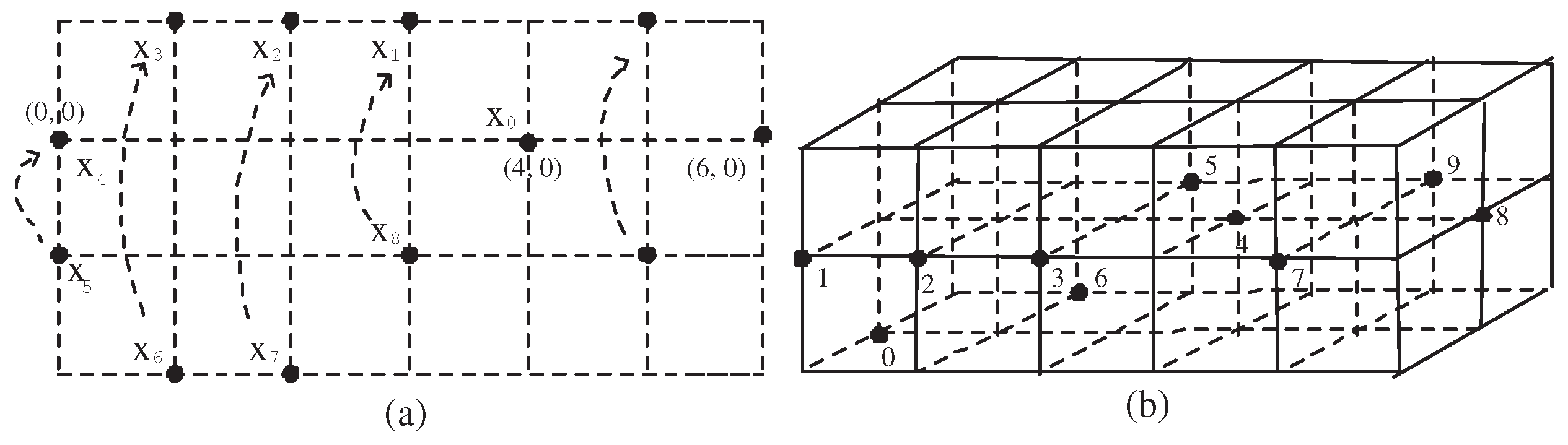
Definition 4

([10,11]). 

(1) 

$MS{S}_6(\subset {\mathbb{Z}}^3)$ is 6-isomorphic to $(X,6)$, where $X:={[-1,1]}_{\mathbb{Z}}^3\backslash \left\{0_3\right\}$, i.e., $MS{S}_6{\approx }_6{[-1,1]}_{\mathbb{Z}}^3\backslash \left\{0_3\right\}$, where $0_3:=(0,0,0)$ (see Figure 4a).

(2) 

$MS{S}_{18}^{\prime }{\approx }_{18}(Y,18)$, where $Y:=\{p\in {\mathbb{Z}}^3 | d(p,0_3)=1\}$ (see Figure 5b(1)), d is the Euclidean distance in ${\mathbb{R}}^3$.

(3) 

$MS{S}_{18}{\approx }_{18}(Z,18)$ (see Figure 5a(1)), where $Z:=(MS{C}_8\times \left\{1\right\})\cup (Int(MS{C}_8)\times \{0,2\})$ [10,11], $MSC:=\{(0,0,),(1,\pm 1),(2,\pm 1),(3,0)\}$, and $Int(MSC):=\{(1,0),(2,0)\}$.

(4) 

$MS{S}_{26}^{\prime }:=MS{S}_{18}^{\prime }$.

Remark 10

 ([10,11]).

(1)

$MS{S}_6$ is not 6-contractible.

(2)

$MS{S}_{18}^{\prime }$ and $MS{S}_{18}$ are considered in the digital pictures $({\mathbb{Z}}^3,18,6,MS{S}_{18}^{\prime })$ and $({\mathbb{Z}}^3,18,6,MS{S}_{18})$, respectively. Besides, each of them is 18-contractible.

(3)

$MS{S}_{26}^{\prime }:=MS{S}_{18}^{\prime }$ is 26-contractible [10,11] and is a minimal simple closed 26-surface (see Figure 5b(1)).

Indeed, each $MS{S}_{18}^{\prime }$ and $MS{S}_{18}$ are 18-contractible [10,11]. In addition, we see that $MS{S}_6$ is simply 6-connected [10].

When studying $S_k\in {\mathbb{Z}}^3$, $k\in \{6,18,26\}$, we should assume $S_k$, $k\in \{6,18,26\}$ in the binary digital picture such as $({\mathbb{Z}}^3,k,\overline{k},S_k)$, where $(S_k,k)$ and $({\mathbb{Z}}^3\backslash S_k,\overline{k})$ are assumed. For instance,

$$\{({\mathbb{Z}}^3,26,6,S_{26}),({\mathbb{Z}}^3,18,6,S_{18}),({\mathbb{Z}}^3,6,26,S_6)\}.$$

(43)

Finally, we assume the following $({\mathbb{Z}}^3,26,6,MS{S}_{26}^{\prime })$, $({\mathbb{Z}}^3,6,26,MS{S}_6)$, $({\mathbb{Z}}^3,18,6,MS{S}_{18}^{\prime })$, and $({\mathbb{Z}}^3,18,6,MS{S}_{18})$ [11].

Let us now investigate the number of 2-components of $F(Co{n}_6(MS{S}_6))$.

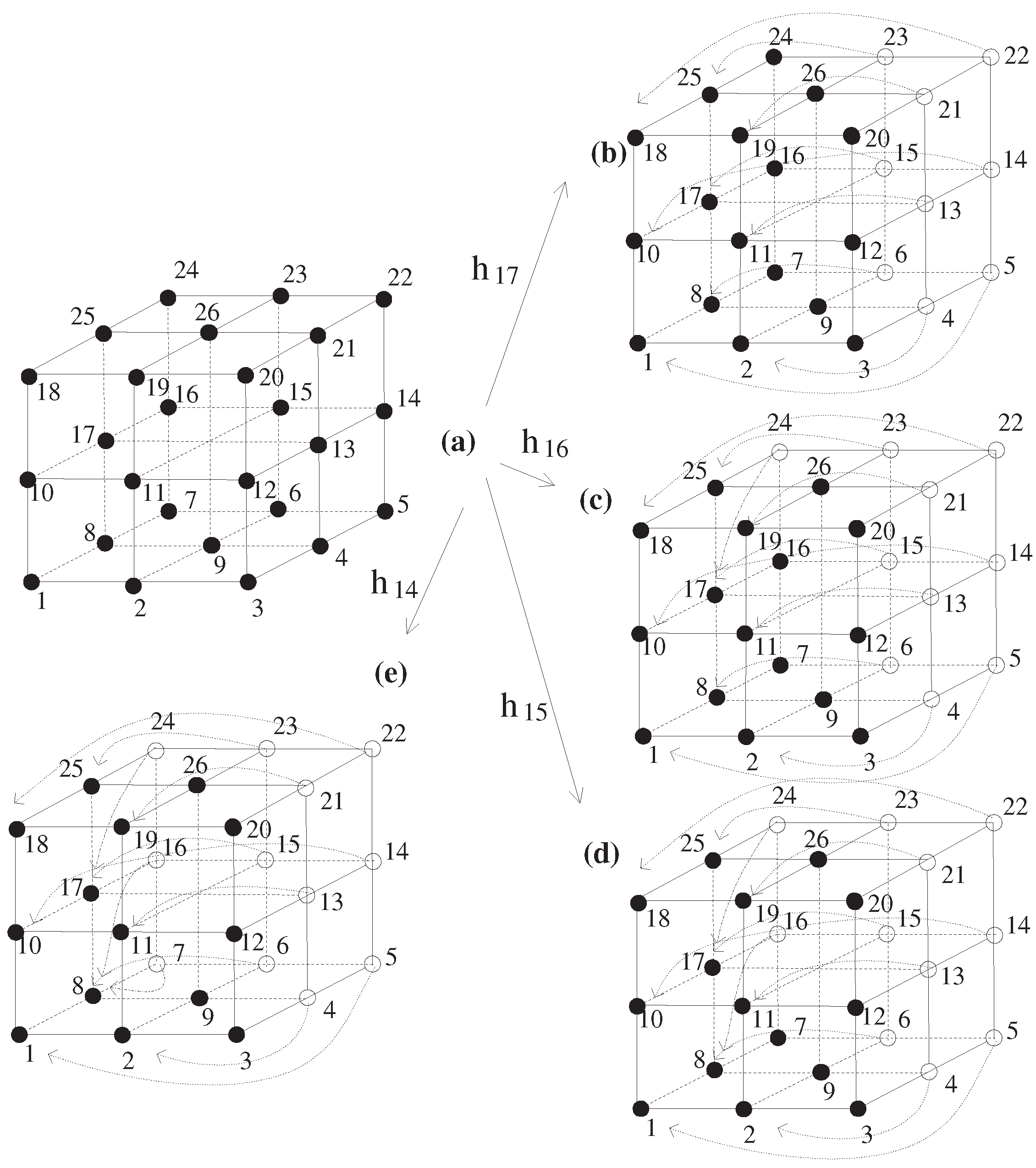
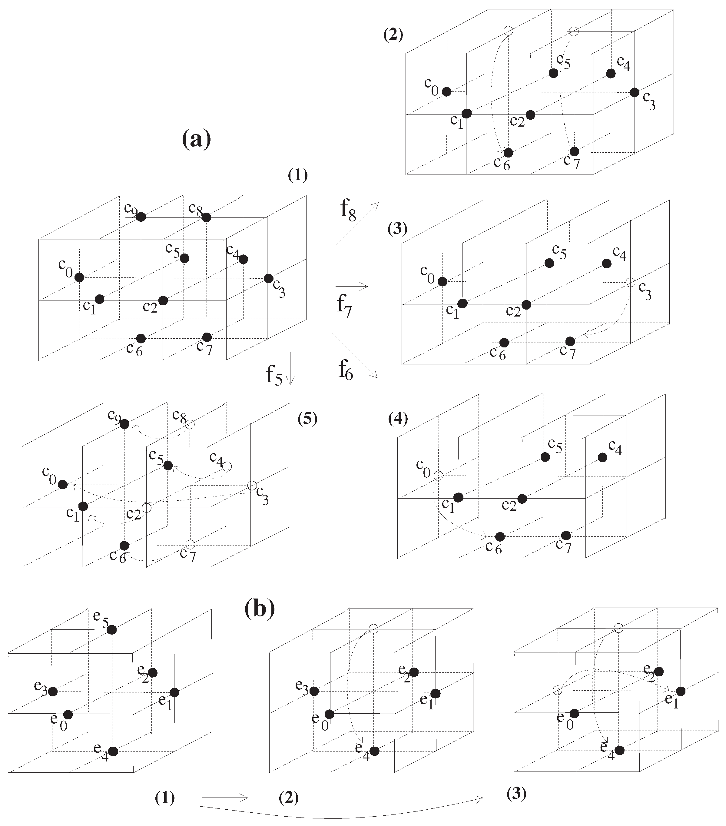
Theorem 14.

$F(Co{n}_6(MS{S}_6))$ is not perfect, i.e., $F(Co{n}_6(MS{S}_6))={[0,17]}_{\mathbb{Z}}\cup \left\{26\right\}$, which has two 2-components.

Proof. 

Let $MS{S}_6:={[1,26]}_{\mathbb{Z}}$ in Figure 4 (for convenience, $MS{S}_6$ is described by using the number $t\in {[1,26]}_{\mathbb{Z}}$). Further consider a 6-continuous self-map f such that $Fix{(f)}^{♯}=17$ (see the map described in Figure 4((a) → (b)). In view of Proposition 1, we observe that there is no $g\in Co{n}_6(MS{S}_6)$ such that $18\le Fix{(g)}^{♯}\le 25$. However, there are many 6-continuous self-maps $h_i$ of $MS{S}_6$ such that $0\le i\le 17$, where $Fix{(h_i)}^{♯}:=i$. To be precise, as shown in Figure 4 (see (a) →(b)), consider the following 6-continuous self-map $h_{17}$ of $MS{S}_6$ such that $Fix{(h_{17})}^{♯}=17$. To be specific,

$$\left\{\begin{array}{l}{h}_{17}(4)=2,h_{17}(5)=1,h_{17}(6)=8,h_{17}(13)=11,h_{17}(14)=10,\\ h_{17}(15)=17,h_{17}(21)=19,h_{17}(22)=18,h_{17}(23)=25, \mathrm{and}\\ h_{17}(x)=x, \mathrm{where} x\in MS{S}_6\backslash \{4,5,6,13,14,15,21,22,23\}.\end{array}\right.$$

Similarly, we also have 6-continuous self-maps $h_i$ of $MS{S}_6$ such that $1\le i\le 16$ such that $Fix{(h_i)}^{♯}:=i$, as follows (see $h_{16}$ in Figure 4((a)→(c), $h_{15}$ in Figure 4((a)→(d), $h_{14}$ in Figure 4((a)→(e), and so on): To be specific,

$$\left\{\begin{array}{l}{h}_{16}\left(24\right)=17\mathrm{and}{h}_{16}{|}_{MS{S}_6\backslash \left\{24\right\}}\left(x\right)=h_{17}\left(x\right),\mathrm{where}x\in MS{S}_6\backslash \left\{24\right\},\\ h_{15}\left(16\right)=8\mathrm{and}{h}_{15}{|}_{MS{S}_6\backslash \left\{16\right\}}\left(x\right)=h_{16}\left(x\right),\mathrm{where}x\in MS{S}_6\backslash \left\{16\right\},\\ h_{14}\left(7\right)=8\mathrm{and}{h}_{14}{|}_{MS{S}_6\backslash \left\{7\right\}}\left(x\right)=h_{15}\left(x\right),\mathrm{where}x\in MS{S}_6\backslash \left\{7\right\},\\ h_{13}\left(20\right)=11\mathrm{and}{h}_{13}{|}_{MS{S}_6\backslash \left\{20\right\}}\left(x\right)=h_{14}\left(x\right),\mathrm{where}x\in MS{S}_6\backslash \left\{20\right\},\\ h_{12}\left(12\right)=2\mathrm{and}{h}_{12}{|}_{MS{S}_6\backslash \left\{12\right\}}\left(x\right)=h_{13}\left(x\right),\mathrm{where}x\in MS{S}_6\backslash \left\{12\right\},\\ h_{11}\left(3\right)=2\mathrm{and}{h}_{11}{|}_{MS{S}_6\backslash \left\{3\right\}}\left(x\right)=h_{12}\left(x\right),\mathrm{where}x\in MS{S}_6\backslash \left\{3\right\},\\ h_{10}\left(26\right)=18\mathrm{and}{h}_{10}{|}_{MS{S}_6\backslash \left\{26\right\}}\left(x\right)=h_{11}\left(x\right),\mathrm{where}x\in MS{S}_6\backslash \left\{26\right\},\\ h_9\left(9\right)=1\mathrm{and}{h}_9{|}_{MS{S}_6\backslash \left\{9\right\}}\left(x\right)=h_{10}\left(x\right),\mathrm{where}x\in MS{S}_6\backslash \left\{9\right\},\\ h_8\left(25\right)=10\mathrm{and}{h}_8|MS{S}_6\backslash \left\{25\right\}\left(x\right)=h_9\left(x\right),\mathrm{where}x\in MS{S}_6\backslash \left\{25\right\},\\ \cdots \\ h_1\left(MS{S}_6\right)=\left\{1\right\}.\end{array}\right.$$

Therefore, we obtain $F(Co{n}_6(MS{S}_6))={[0,17]}_{\mathbb{Z}}\cup \left\{26\right\}$. □

Let us now recall the 18-contractibility of $MS{S}_{18}^{\prime }$ and $MS{S}_{18}$ (see also Theorem 6 and Figure 2 of [11]), as follows.

Lemma 3

([11]). Each $MS{S}_{18}^{\prime }$ and $MS{S}_{18}$ are 18-contractible.

Let us now examine if each of $F(Co{n}_{18}(Y))$ and $F(Co{n}_{26}(MS{S}_{26}^{\prime }))$ is perfect, where $Y\in \{MS{S}_{18},MS{S}_{18}^{\prime }\}$.

Theorem 15. 

(1)

$F(Co{n}_{18}(MS{S}_{18}))$ is not perfect, i.e., $F(Co{n}_{18}(MS{S}_{18}))={[0,8]}_{\mathbb{Z}}\cup \left\{10\right\}$, which has two 2-components.

(2)

$F(Co{n}_{18}(MS{S}_{18}^{\prime }))$ is perfect.

(3)

$F(Co{n}_{26}(MS{S}_{26}^{\prime }))$ is perfect.

Proof. 

(1) It is clear that $9\notin F(Co{n}_{18}(MS{S}_{18}))$ because there is no 18-continuous self-map f of $MS{S}_{18}:=\{c_i | i\in {[0,9]}_{\mathbb{Z}}\}$ (see Figure 5a(1) and Lemma 2 and Theorem 4) such that ${(Im(f))}^{♯}=9$ (see also Proposition 1). Naively, it is clear that there is no $f\in Co{n}_{18}(MS{S}_{18})$ such that $Im(f)=MS{S}_{18}\backslash \left\{p\right\}$ for a point $p\in MS{S}_{18}$ contrary to Proposition 1 so that there is no 18-continuous self-map f of $MS{S}_{18}$ such that $Fix{(f)}^{♯}=9$. However, there are many 18-continuous self-maps of $MS{S}_{18}$ such that $Im{(f)}^{♯}\le 8$ and further, $Fix{(f)}^{♯}\le 8$.

To be specific, first, consider the 18-continuous self-map $f_8$ of $MS{S}_{18}$ in Figure 5a such that $Fix{(f_8)}^{♯}=8$ (see Figure 5a (1) → (2)), i.e.,

$$f_8(c_9)=c_6,f_8(c_8)=c_7, \mathrm{and} f_8(x)=x,x\in MS{S}_{18}\backslash \{c_8,c_9\}.$$

Second, consider the 18-continuous self-map $f_7$ of $MS{S}_{18}$ in Figure 6a such that $Fix{(f_7)}^{♯}=7$ (see Figure 5a (1) → (3)), i.e.,

$$f_7(c_9)=c_6,f_7(\{c_3,c_8\})=\left\{c_7\right\}, \mathrm{and} f_7(x)=x,x\in MS{S}_{18}\backslash \{c_8,c_9,c_3\}.$$

Third, consider the 18-continuous self-map $f_6$ of $MS{S}_{18}$ in Figure 5a such that $Fix{(f_6)}^{♯}=6$ (see Figure 5a (1) → (4)), i.e.,

$$\left\{\begin{array}{l}{f}_6(\{c_0,c_9\})=\left\{c_6\right\},f_6(\{c_3,c_8\})=\left\{c_7\right\}, \mathrm{and}\\ f_6(x)=x,x\in MS{S}_{18}\backslash \{c_0,c_3,c_8,c_9\}.\end{array}\right.$$

Fourth, consider the 18-continuous self-map $f_5$ of $MS{S}_{18}$ in Figure 5a such that $Fix{(f_5)}^{♯}=5$ (see Figure 5a(1) → (5)), i.e.,

$$\left\{\begin{array}{l}{f}_5(c_3)=c_0,f_5(c_2)=c_1,f_5(c_7)=c_6,f_5(c_4)=c_5,f_5(c_8)=c_9, \mathrm{and}\\ f_5(x)=x,x\in MS{S}_{18}\backslash \{c_2,c_3,c_4,c_7,c_8\}.\end{array}\right.$$

Fifth, based on this map $f_5$, further consider the 18-continuous self-map $f_4$ of $MS{S}_{18}$ in Figure 6a such that $Fix{(f_4)}^{♯}=4$, i.e.,

$$\left\{\begin{array}{l}{f}_4(c_2)=c_1,f_4(\{c_3,c_6,c_7\})=\left\{c_0\right\},f_4(c_4)=c_5,f_4(c_8)=c_9, \mathrm{and}\\ f_4(x)=x,x\in MS{S}_{18}\backslash \{c_2,c_3,c_4,c_6,c_7,c_8\}.\end{array}\right.$$

Similarly, motivated by the establishment of $f_4$, we obtain an 18-continuous self-map $f_i$ of $MS{S}_{18}$ in Figure 5a satisfying $Fix{(f_i)}^{♯}=i,i\in \{1,2,3\}$. Furthermore, as only a digital image with a singleton has the fixed point property [11,15,26], it is clear that $0\in F(Co{n}_{18}(MS{S}_{18}))$. Based on these cases, we obtain $F(Co{n}_{18}(MS{S}_{18}))={[0,8]}_{\mathbb{Z}}\cup \left\{10\right\}$, which completes the proof.

(2) We prove the assertion using Theorem 4. First, consider the 18-continuous self-map $g_5$ of $MS{S}_{18}^{\prime }$ in Figure 5b such that $Fix{(g_5)}^{♯}=5$, i.e.,

$$g_5(e_5)=e_4 \mathrm{and} g_5(x)=x,x\in MS{S}_{18}^{\prime }\backslash \left\{e_5\right\}.$$

Second, motivate by the maps $f_i,i\in [1,5]$ in (1) above, we easily establish certain 18-continuous self-maps $g_i$ of $MS{S}_{18}^{\prime }$ in Figure 5b(see (1) →(2) and (1) →(3)) such that ${(Fix(g_i))}^{♯}=i,i\in {[1,5]}_{\mathbb{Z}}$.

Finally, we obtain $F(Co{n}_{18}(MS{S}_{18}^{\prime }))={[0,6]}_{\mathbb{Z}}$.

(3) Motivated by the proof of (2) above, using Theorem 4, we complete the proof. □

By Lemma 3 and Theorem 15(1), the following is obtained.

Remark 11.

Although $MS{S}_{18}$ is 18-contractible, $F(Co{n}_{18}(MS{S}_{18}))$ is not perfect

As proven in Theorem 15(1), though $F(Co{n}_{18}(MS{S}_{18}))$ is not perfect, we obtain the following:

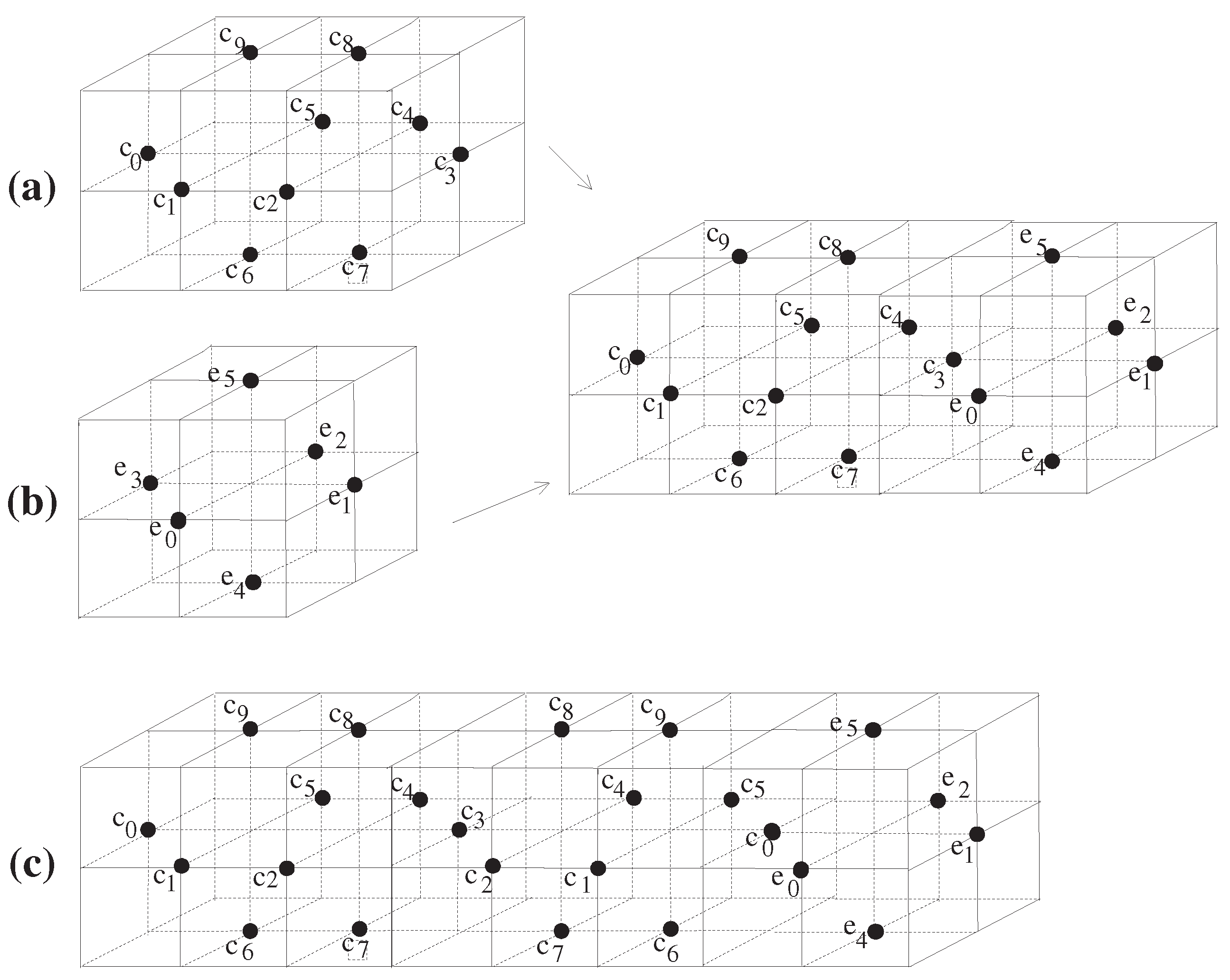
Theorem 16.

$F(Co{n}_{18}(MS{S}_{18}\vee MS{S}_{18}^{\prime }))$ is perfect.

Proof. 

Let $A:=MS{S}_{18}:={(c_i)}_{i\in {[0,9]}_{\mathbb{Z}}}$ and $B:=MS{S}_{18}^{\prime }:={(b_i)}_{i\in {[0,5]}_{\mathbb{Z}}}$ and $\left\{p\right\}:=A\cap B$, i.e., $p:=c_3=e_3$ (see Figure 6a(1),b(1)). Regarding $F(Co{n}_{18}(MS{S}_{18}\vee MS{S}_{18}^{\prime }))$, it is sufficient to consider the following 18-continuous self-maps of $MS{S}_{18}\vee MS{S}_{18}^{\prime }$ such that

$$\left\{\begin{array}{l}(1) f \mathrm{satisfies} f(A)\subset A \mathrm{or} f(A)\subset B, \mathrm{and} f|B(x)=x,\\ (2) f \mathrm{satisfies} f(B)⊊B \mathrm{or} f(B)\subset A \mathrm{and} f|A(x)=x,\\ (3) f \mathrm{satisfies} f(A)⊊A \mathrm{and} f(B)⊊B, \mathrm{and}\\ (4) \mathrm{only} \mathrm{a} \mathrm{digital} \mathrm{image} \mathrm{with} \mathrm{a} \sin \mathrm{gleton} \mathrm{has} \mathrm{the} \mathrm{fixed} \mathrm{point} \mathrm{property}.\end{array}\right\}$$

(44)

According to (44), we now investigate $F(Co{n}_{18}(A\vee B))$ with the following four cases.

First, according to (44)(1), we obtain

$${[6,13]}_{\mathbb{Z}}\cup \left\{15\right\}\subset F(Co{n}_{18}(A\vee B)).$$

(45)

Second, according to (44)(2), we have

$${[10,15]}_{\mathbb{Z}}\subset F(Co{n}_{18}(A\vee B)).$$

(46)

Third, according to (44)(3), we obtain

$${[1,12]}_{\mathbb{Z}}\subset F(Co{n}_{18}(A\vee B)).$$

(47)

Fourth, according to (44)(4), we obtain

$$\left\{0\right\}\subset F(Co{n}_{18}(A\vee B)).$$

(48)

Therefore, by these four quantities from (45), (46), (47), and (48) as subsets of $F(Co{n}_{18}(A\vee B))$, we obtain

$$F(Co{n}_{18}(C\vee D))={[0,15]}_{\mathbb{Z}}. \square$$

Owing to Theorem 16, it turns out that while $F(Co{n}_{18}(MS{S}_{18}))$ is not perfect, $F(Co{n}_{18}(MS{S}_{18}\vee MS{S}_{18}^{\prime }))$ is perfect. □

Theorem 17.

$F(Co{n}_{18}(MS{S}_{18}\vee MS{S}_{18}))$ is not perfect and has two 2-components.

Proof. 

Using a method similar to the approach of (44), we consider the following 18-continuous self-maps f of $MS{S}_{18}\vee MS{S}_{18}$ such that

$$\left\{\begin{array}{l}(1) f \mathrm{satisfies} f(MS{S}_{18})\subset MS{S}_{18}{ \mathrm{and} f|}_{MS{S}_{18}}(x)=x,\\ (2) \mathrm{for} \mathrm{each} MS{S}_{18}, f \mathrm{satisfies} f(MS{S}_{18})⊊MS{S}_{18} \mathrm{and}\\ (3) \mathrm{only} \mathrm{a} \mathrm{digital} \mathrm{image} \mathrm{with} \mathrm{a} \sin \mathrm{gleton} \mathrm{has} \mathrm{the} \mathrm{fixed} \mathrm{point} \mathrm{property}.\end{array}\right\}$$

(49)

From (49)(1), we obtain the following,

$${[10,17]}_{\mathbb{Z}}\cup \left\{19\right\}\subset F(Co{n}_{18}(MS{S}_{18}\vee MS{S}_{18})).$$

(50)

From (49)(2)–(3), and further, motivated by the map $f_5$ of Figure 5 we obtain the following,

$${[0,15]}_{\mathbb{Z}}\subset F(Co{n}_{18}(MS{S}_{18}\vee MS{S}_{18})).$$

(51)

In view of (50) and (51), by

Lemma 2, we obtain

$$F(Co{n}_{18}(MS{S}_{18}\vee MS{S}_{18}))={[0,17]}_{\mathbb{Z}}\cup \left\{19\right\},$$

which implies that $F(Co{n}_{18}(MS{S}_{18}\vee MS{S}_{18}))$ is not perfect because $18\notin F(Co{n}_{18}(MS{S}_{18}\vee MS{S}_{18}))$. □

Corollary 3.

$F(Co{n}_{18}(MS{S}_{18}\vee MS{S}_{18}\vee MS{S}_{18}^{\prime }))$ is perfect.

Proof. 

From Theorem 17, as

$$F(Co{n}_{18}(MS{S}_{18}\vee MS{S}_{18}))={[0,17]}_{\mathbb{Z}}\cup \left\{19\right\},$$

after joining $MS{S}_{18}^{\prime }$ onto $MS{S}_{18}\vee MS{S}_{18}$ (see Figure 6c), we produce the digital wedge $(MS{S}_{18}\vee MS{S}_{18}\vee MS{S}_{18}^{\prime },18)$. Finally, by Theorem 4, we have

$$F(Co{n}_{18}(MS{S}_{18}\vee MS{S}_{18}\vee MS{S}_{18}^{\prime }))={[0,24]}_{\mathbb{Z}},$$

which is perfect. □

7. Conclusions

As conclusions, given $C_k^{n,l_i},i\in \{1,2\}$, we formulated $F(Co{n}_k(C_k^{n,l_1}\vee C_k^{n,l_2}))$ without any limitation of the numbers $l_i,i\in \{1,2\}$, which are either odd or even. In one of the key works, we were able to explore some properties of several types of digital k-surfaces motivated by the digital k-surfaces [8,10,11,27] and study some properties of fixed point sets of them. Eventually, it turns out that there are non-perfectness of $F(Co{n}_{18}(MS{S}_{18}\vee MS{S}_{18}))$ and $F(Co{n}_6(MS{S}_6))$ and perfectness of $F(Co{n}_{18}(MS{S}_{18}\vee MS{S}_{18}\vee MS{S}_{18}^{\prime }))$, which can be used in studying both fixed point theory in a $DTC$ setting and digital geometry.

The study of a certain connection between fixed point sets of typical topological spaces X in the n-dimensional Euclidean space and those of the digitized space (or digital image) of X plays an important role in both pure topology and digital topology. Based on the study of fixed point sets in the present paper, we can recognize the quantity of fixed points of a given digital object and classify digital objects because the alignment is a digital topological invariant. The obtained results in the $DTC$ setting can be applied to the fields of chemistry, physics, computer sciences, and so on. In particular, this approach can be extremely useful in the fields of classifying molecular structures, computer graphics, image processing [28], approximation theory, game theory, mathematical morphology [29], fractal image compression [30], digitization, robotics [31], rough set theory, and so forth.