Martingale Approach to Derive Lundberg-Type Inequalities

Abstract

In this paper, we find the upper bound for the tail probability $\mathbb{P}\left({sup}_{n⩾0}{\sum }_{\mathrm{I}=1}^n{\xi }_{\mathrm{I}}>x\right)$ with random summands ${\xi }_1,{\xi }_2,\dots$ having light-tailed distributions. We find conditions under which the tail probability of supremum of sums can be estimated by quantity ${\varrho }_{1}exp\{-{\varrho }_{2}x\}$ with some positive constants ${\varrho }_1$ and ${\varrho }_2$. For the proof we use the martingale approach together with the fundamental Wald’s identity. As the application we derive a few Lundberg-type inequalities for the ultimate ruin probability of the inhomogeneous renewal risk model.

1. Introduction

Let $\{{\xi }_1,{\xi }_2,\dots \}$ be a sequence of independent and real-valued random variables (r.v.s). Let ${\mathcal{S}}_0=0$, ${\mathcal{S}}_n={\xi }_1+{\xi }_2+\dots +{\xi }_n$ for all $n\in \mathbb{N}$ and ${\mathcal{M}}_{\infty }=sup\{{\mathcal{S}}_0,{\mathcal{S}}_1,{\mathcal{S}}_2,\dots \}$. In 1997, Sgibnev generalized results of Kiefer and Wolfowitz [1] by obtaining the upper bound for submultiplicative moment $\mathbb{E}\phi \left({\mathcal{M}}_{\infty }\right)$ in the case of independent and identically distributed (i.i.d.) r.v.s. In Theorem 2 of [2] the following assertion is presented.

Theorem 1.

Let $\{{\xi }_1,{\xi }_2,\dots \}$ be a sequence of i.i.d. r.v.s with a common distribution function (d.f.) F. Let φ be a non-decreasing function defined on $[0,\infty )$ such that $\phi \left(0\right)=1$ and $\phi (x+y)⩽\phi \left(x\right)\phi \left(y\right)$ for all $x,y\in [0,\infty )$. Then $\mathbb{E}\phi \left({\mathcal{M}}_{\infty }\right)<\infty$ under the following three conditions:

$$\begin{array}{cc}\hfill \left(\mathrm{i}\right)& \mathbb{E}{\xi }_1<0,\hfill \\ \hfill \left(\mathrm{ii}\right)& {\int }_0^{\infty }\phi \left(x\right)\overline{F}\left(x\right)\mathrm{d}x<\infty ,\hfill \\ \hfill \left(\mathrm{iii}\right)& \mathrm{if}r=r\left(\phi \right):=\underset{x\to \infty }{lim}\frac{log\phi \left(x\right)}{x}>0,\mathrm{then}\mathbb{E}\left({\mathrm{e}}^{r{\xi }_1}\right)<1.\hfill \end{array}$$

In the case of exponential function $\phi$, Theorem 1 implies the following upper estimation for the tail probability of r.v. ${\mathcal{M}}_{\infty }$.

Corollary 1.

Let $\{{\xi }_1,{\xi }_2,\dots \}$ be a sequence of i.i.d. r.v.s. If $\mathbb{E}{\xi }_1<0$ and $\mathbb{E}{\mathrm{e}}^{h{\xi }_1}<\infty$ for some positive h then there exist positive constants ${\varrho }_1$ and ${\varrho }_2$ such that

$$\mathbb{P}\left({\mathcal{M}}_{\infty }>x\right)⩽{\varrho }_1{\mathrm{e}}^{-{\varrho }_{2}x}$$

(1)

for all nonnegative x.

If a sequence $\{{\xi }_1,{\xi }_2,\dots \}$ consists of independent but possibly differently distributed r.v.s, then the similar estimate to that in (1) also holds. The following assertion is proved in [3] (see Lemma 1).

Theorem 2.

Let $\{{\xi }_1,{\xi }_2,\dots \}$ be a sequence of independent r.v.s such that

$$\begin{array}{cc}\hfill \left(\mathrm{i}\right)& \underset{k\in \mathbb{N}}{sup}\mathbb{E}\left({\mathrm{e}}^{h{\xi }_k}\right)<\infty \mathit{for}\mathit{some}h>0,\hfill \\ \hfill \left(\mathrm{ii}\right)& \underset{u\to \infty }{lim}\underset{k\in \mathbb{N}}{sup}\mathbb{E}\left(|{\xi }_k|1{\mathrm{I}}_{\{{\xi }_k⩽-u\}}\right)=0,\hfill \\ \hfill \left(\mathrm{iii}\right)& \underset{n\to \infty }{lim\; sup}\frac{1}{n}\sum _{k=1}^n\mathbb{E}{\xi }_k<0.\hfill \end{array}$$

Then the estimate (1) holds for all positive x and some positive constants ${\varrho }_1$ and ${\varrho }_2$.

In Theorem 3 of [4] the following more general assertion was proved using classical ideas of Chernoff [5] and Hoeffding [6].

Theorem 3.

Let $\{{\xi }_1,{\xi }_2,\dots \}$ be a sequence of independent r.v.s such that:

$$\begin{array}{ccc}& \left(\mathrm{i}\right)& \frac{1}{n}\sum _{k=1}^n\mathbb{E}{\xi }_k⩽-a\mathrm{if}n⩾b,\hfill \\ & \left(\mathrm{ii}\right)& \underset{n⩾b}{sup}\frac{1}{n}\sum _{k=1}^n\mathbb{E}\left(|{\xi }_k|1{\mathrm{I}}_{\{{\xi }_k⩽-c\}}\right)⩽\epsilon ,\hfill \\ & \left(\mathrm{iii}\right)& \underset{n⩾b}{sup}\frac{1}{n}\sum _{k=1}^n\left(\mathbb{P}({\xi }_k⩽0)+\mathbb{E}\left({\mathrm{e}}^{h{\xi }_k}1{\mathrm{I}}_{\{{\xi }_k>0\}}\right)\right)⩽d_1,\hfill \\ & \left(\mathrm{i}\mathrm{v}\right)& \underset{1⩽n⩽b-1}{max}\frac{1}{n}\sum _{k=1}^n\left(\mathbb{P}({\xi }_k⩽0)+\mathbb{E}\left({\mathrm{e}}^{h{\xi }_k}1{\mathrm{I}}_{\{{\xi }_k>0\}}\right)\right)⩽d_2,\hfill \end{array}$$

for some $a>0$, $b\in \mathbb{N}$, $c>0$, $\epsilon ⩾0$, $h>0$, $d_1⩾1$ and $d_2⩾1$.

If

$$-\Delta :=\epsilon +\delta h{d}_{1}max\left\{\frac{c^2}{2},\frac{2}{h^2}\right\}-a<0$$

(2)

with $\delta \in (0,1/2)$, then

$$\mathbb{P}\left({\mathcal{M}}_{\infty }>x\right)⩽c_1{\mathrm{e}}^{-\delta hx},x⩾0,$$

where

$$c_1=\left(\sum _{n=1}^{b-1}{d}_2^n+\frac{exp\{-\delta h\Delta b\}}{1-exp\{-\delta h\Delta \}}\right).$$

It should be noted that conditions of Theorem 3 are weaker than the conditions of Theorem 2. In addition, the assertion of Theorem 3 provides an algorithm to calculate two positive constants controlling the exponential upper bound. For this reason, conditions of the last theorem have more explicit form.

In this paper we extend the above results by deriving the more precise upper bounds for probability $\mathbb{P}\left({\mathcal{M}}_{\infty }>x\right)$ under less restrictive requirements. In addition, from these upper bounds we derive the so called Lundberg-type exponential estimates for ruin probabilities of the nonhomogeneous renewal risk models. Results on upper bounds for $\mathbb{P}\left({\mathcal{M}}_{\infty }>x\right)$ are presented in Section 2, and the versions of the Lundberg-type inequalities are given in Section 3. Section 4 deals with proofs of the main results, and finally, Section 5 addresses to several applications of the results obtained.

It should be noted that the problem under consideration and the method used are related with the problem of upper bound for probability $\mathbb{P}(S_n>x)$, where $S_n$ is a sum of independent or dependent random variables. It is natural that for probability $\mathbb{P}(S_n>x)$ more sharp upper bounds can be obtained comparing with the upper bound for $\mathbb{P}({max}_{1⩽k⩽n}{S}_k>x)$. The pioneer exponential-type inequalities for probability $\mathbb{P}(S_n>x)$ were derived by Bernstein [7,8] and later were improved and generalized by many authors, see [6,9,10,11,12,13,14,15], for instance. The boundedness of summands in $S_n$ is a key requirement in these papers to get sharp exponential-type upper bounds. Upper bound for probability $\mathbb{P}({max}_{1⩽k⩽n}{S}_k>x)$ can be derived from the upper estimates of $\mathbb{P}(S_n>x,\mathcal{C})$ with a suitable condition $\mathcal{C}$. Such a way is described in detail by Fan et al. [12] and in references therein. Unfortunately, the derived upper exponential-type estimates for $\mathbb{P}(S_n>x,\mathcal{C})$ “work” under quite restrictive requirements for summands of sum $S_n$. The main object of our research is the ruin probability of the renewal risk model. In order to obtain a good and general upper bound of this probability, we use the estimate of probability $\mathbb{P}({max}_{1⩽k⩽n}{S}_k>x)$ presented in Lemma 1. In this lemma the requirements for summands of $S_n$ are minimal.

2. Upper Bounds for Tail of Maximum of Sums

The first theorem of this section gives the upper estimate for probability $\mathbb{P}\left({\mathcal{M}}_{\infty }>x\right)$ under less requirements than in Theorems 2 and 3 by supposing that random variables ${\xi }_1,{\xi }_2,\dots$ satisfy the net profit condition, have a finite exponential moment and a negligible left tail on average.

Theorem 4.

Let $\{{\xi }_1,{\xi }_2,\dots \}$ be a sequence of independent and possibly differently distributed r.v.s. If the following three conditions are satisfied

$$\begin{array}{cc}\hfill \left(\mathrm{i}\right)& \underset{n\to \infty }{lim\; sup}\frac{1}{n}\sum _{k=1}^n\mathbb{E}\left({\mathrm{e}}^{h{\xi }_k}\right)<\infty \mathit{for}\mathit{some}h>0,\hfill \\ \hfill \left(\mathrm{ii}\right)& \underset{n\to \infty }{lim\; sup}\frac{1}{n}\sum _{k=1}^n\mathbb{E}{\xi }_k<0,\hfill \\ \hfill \left(\mathrm{iii}\right)& \underset{\begin{array}{c}u\to \infty \\ n\to \infty \end{array}}{lim\; sup}\frac{1}{n}\sum _{k=1}^n\mathbb{E}\left(|{\xi }_k|1{\mathrm{I}}_{\{{\xi }_k⩽-u\}}\right)=0,\hfill \end{array}$$

then the estimate (1) holds for all positive x and some positive constants ${\varrho }_1$ and ${\varrho }_2$.

The second theorem provides an algorithm to obtain numerical expressions of constants ${\varrho }_1$ and ${\varrho }_2$ in the estimate (1). The assertion of theorem below is similar to that in Theorem 3. However, we derive more precise expressions of constants using the sharp initial inequality of Lemma 1 below.

Theorem 5.

Let $\{{\xi }_1,{\xi }_2,\dots \}$ be a sequence of independent r.v.s such that:

$$\begin{array}{ccc}& \left(\mathrm{i}\right)& \frac{1}{n}\sum _{k=1}^n\mathbb{E}{\xi }_k⩽-a,\hfill \\ & \left(\mathrm{ii}\right)& \frac{1}{n}\sum _{k=1}^n\mathbb{E}\left(|{\xi }_k|1{\mathrm{I}}_{\{{\xi }_k⩽-c\}}\right)⩽\epsilon ,\hfill \\ & \left(\mathrm{iii}\right)& \frac{1}{n}\sum _{k=1}^n\left(\mathbb{P}({\xi }_k⩽0)+\mathbb{E}\left(\left({\mathrm{e}}^{h{\xi }_k}-{\mathrm{e}}^{h{\xi }_k/2}\right)1{\mathrm{I}}_{\{{\xi }_k>0\}}\right)\right)⩽d,\hfill \end{array}$$

for $n⩾b$, $a>0$, $b\in \mathbb{N}$, $c>0$, $\epsilon ⩾0$, $h>0$, $d⩾1$. Let, in addition:

$$\begin{array}{c}\hfill \left(\mathrm{iv}\right)\underset{1⩽n⩽b-1}{max}\prod _{k=1}^n\left(\mathbb{P}({\xi }_k⩽0)+\mathbb{E}\left({\mathrm{e}}^{h{\xi }_k}1{\mathrm{I}}_{\{{\xi }_k>0\}}\right)\right)⩽D\end{array}$$

for $D⩾1$.

If

$$\epsilon +\delta hdmax\left\{\frac{c^2}{2},\frac{2}{h^2}\right\}-a⩽0$$

(3)

with some $\delta \in (0,1/2)$, then for all positive x

$$\mathbb{P}\left({\mathcal{M}}_{\infty }>x\right)⩽D{\mathrm{e}}^{-\delta hx}.$$

(4)

The last theorem shows what upper bound can be derived for tail of maximum of sums in the case when the cumulant generating functions (see [16], for instance) can be successfully estimated for all r.v.s $\{{\xi }_1,{\xi }_2,\dots \}$.

Theorem 6.

Let $\{{\xi }_1,{\xi }_2,\dots \}$ be a sequence of independent r.v.s. If for all $h\in (0,h^{*})$ and $n\in \mathbb{N}$

$$\sum _{k=1}^{n}log\left(\mathbb{E}\left({\mathrm{e}}^{h{\xi }_k}\right)\right)⩽\phi \left(h\right)$$

(5)

with some $h^{*}>0$ and function φ not depending on n, then

$$\mathbb{P}\left({\mathcal{M}}_{\infty }>x\right)⩽exp\left\{-hx+\phi \left(h\right)\right\}$$

(6)

for all positive x and $h\in (0,h^{*})$.

Remark 1.

The last estimation (6) implies the possibility to get more sharp estimate than the standard exponential for $\mathbb{P}\left({\mathcal{M}}_{\infty }>x\right)$. For example, if $\phi \left(x\right)/x<x/2$ for large x, then (6) implies that

$$\mathbb{P}\left({\mathcal{M}}_{\infty }>x\right)⩽exp\{-x^2/2\}$$

for that x.

3. Exponential Estimates for Ruin Probabilities

In this section, we present three corollaries from Theorems 4–6 on the Lundberg-type inequalities for the ultimate ruin probability of an inhomogeneous renewal risk model.

We say that the insurer’s surplus $R\left(t\right)$ varies according to an inhomogeneous renewal risk model (IRRM) if equation

$$R(t,x)=x+pt-\sum _{\mathrm{I}=1}^{\mathsf{\Theta }\left(t\right)}{Z}_{\mathrm{I}}$$

(7)

holds for all $t⩾0$ with the initial insurer’s surplus $x⩾0$, a constant premium rate $p>0$, a sequence of independent, non negative and possibly differently distributed claim amounts $\{Z_1,Z_2,\dots \}$ and with the renewal counting process

$$\mathsf{\Theta }\left(t\right)=\sum _{n=1}^{\infty }1{\mathrm{I}}_{\{{\theta }_1+{\theta }_2+\dots +\theta n⩽t\}},$$

generated by the inter occurrence times $\{{\theta }_1,{\theta }_2,\dots \}$ which form a sequence of independent, non negative, not degenerate at zero and possibly differently distributed r.v.s. In addition, sequences $\{Z_1,Z_2,\dots \}$ and $\{{\theta }_1,{\theta }_2,\dots \}$ are supposed to be independent.

If sequences $\{Z_1,Z_2,\dots \}$ and $\{{\theta }_1,{\theta }_2,\dots \}$ consist of independent and identically distributed (i.i.d.) r.v.s, then the inhomogeneous renewal risk model becomes the homogeneous one.

The ultimate ruin probability (or simply ruin probability)

$$\psi \left(x\right)=\mathbb{P}\left(\underset{t⩾0}{inf}R(t,x)<0\right)$$

and the probability of ruin within time T

$$\psi (x,T)=\mathbb{P}\left(\underset{0⩽t⩽T}{inf}R(t,x)<0\right)$$

are the main characteristics of the renewal risk model.

It is obvious that $\psi (x,T)⩽\psi \left(x\right)$ for all $T⩾0$, $x⩾0$, and

$$\psi \left(x\right)=\mathbb{P}\left(\underset{n⩾1}{sup}\sum _{k=1}^n(Z_k-p{\theta }_k)>x\right)$$

(8)

for all $x⩾0$.

There exist a lot of different papers in which various problems related with $\psi \left(x\right)$ and $\psi (x,T)$ were considered. We refer to only a few of them. For instance, in [17,18,19,20,21], different proofs of the classical Ludberg’s inequality can be found. In [22,23,24,25,26,27,28,29,30,31], the methods are presented for calculation of ruin probabilities and related quantities in the discrete time models. In [32,33,34,35,36,37,38,39,40,41,42], various problems of inhomogeneous and homogeneous renewal risk models related with asymptotic behaviour of ruin probabilities were considered.

The equality (8) shows that results of Theorems 4–6 can be directly applied to derive exponential estimates for $\psi \left(x\right)$ of IRRM which are traditionally called Lundberg-type inequalities. In this section, we present three versions of the Lundberg-type inequality for IRRM.

Corollary 2.

Let $\{Z_1,Z_2,\dots \}$ and $\{{\theta }_1,{\theta }_2,\dots \}$ be two independent sequences of independent and possibly differently distributed r.v.s generating IRRM with premium income rate p. Then

$$\psi \left(x\right)⩽{\kappa }_1{\mathrm{e}}^{-{\kappa }_{2}x}$$

for all $x⩾0$ and some positive constants ${\kappa }_1$ and ${\kappa }_2$ if the following conditions are satisfied

$$\begin{array}{cc}\hfill \left(\mathrm{i}\right)& \underset{n\to \infty }{lim\; sup}\frac{1}{n}\sum _{k=1}^n\mathbb{E}\left({\mathrm{e}}^{h{Z}_k}\right)<\infty \mathit{for}\mathit{some}h>0,\hfill \\ \hfill \left(\mathrm{ii}\right)& \underset{n\to \infty }{lim\; sup}\frac{1}{n}\sum _{k=1}^n\mathbb{E}\left(Z_k-p{\theta }_k\right)<0,\hfill \\ \hfill \left(\mathrm{iii}\right)& \underset{\begin{array}{c}u\to \infty \\ n\to \infty \end{array}}{lim\; sup}\frac{1}{n}\sum _{k=1}^n\mathbb{E}\left({\theta }_{k}1{\mathrm{I}}_{\{{\theta }_k⩾u\}}\right)=0.\hfill \end{array}$$

Corollary 3.

Let $\{Z_1,Z_2,\dots \}$ and $\{{\theta }_1,{\theta }_2,\dots \}$ be two independent sequences of independent and possibly differently distributed r.v.s generating IRRM with premium income rate p such that:

$$\begin{array}{ccc}& \left(\mathrm{i}\right)& \frac{1}{n}\sum _{k=1}^n\mathbb{E}\left(Z_k-p{\theta }_k\right)⩽-A,\hfill \\ & \left(\mathrm{ii}\right)& \frac{1}{n}\sum _{k=1}^n\mathbb{E}\left({\theta }_{k}1{\mathrm{I}}_{\{{\theta }_k⩾C/p\}}\right)⩽\Delta ,\hfill \\ & \left(\mathrm{iii}\right)& \frac{1}{n}\sum _{k=1}^n\left(\mathbb{P}(Z_k-p{\theta }_k⩽0)+\mathbb{E}\left(\left({\mathrm{e}}^{H(Z_k-p{\theta }_k)}\right)1{\mathrm{I}}_{\{Z_k-p{\theta }_k>0\}}\right)\right)⩽d^{*},\hfill \end{array}$$

for $n⩾B$, $A>0$, $B\in \mathbb{N}$, $C>0$, $\Delta ⩾0$, $H>0$, $d^{*}⩾1$. If

$$\begin{array}{ccc}& & \left(\mathrm{iv}\right)\underset{1⩽n⩽B-1}{max}\prod _{k=1}^n\left(\mathbb{P}(Z_k-p{\theta }_k⩽0)+\mathbb{E}\left({\mathrm{e}}^{H(Z_k-p{\theta }_k)}1{\mathrm{I}}_{\{Z_k-p{\theta }_k>0\}}\right)\right)⩽D^{*}\hfill \end{array}$$

for some $D^{*}⩾1$, and

$$\Delta +\delta H{d}^{*}max\left\{\frac{C^2}{2},\frac{2}{H^2}\right\}-A⩽0$$

for some $\delta \in (0,1/2)$, then for all positive x

$$\psi \left(x\right)⩽D^{*}{\mathrm{e}}^{-\delta Hx}.$$

Corollary 4.

Let $\{Z_1,Z_2,\dots \}$ and $\{{\theta }_1,{\theta }_2,\dots \}$ be two independent sequences of independent and possibly differently distributed r.v.s generating IRRM with premium income rate p. If for all $h\in (0,h^{*})$ and $n\in \mathbb{N}$

$$\sum _{k=1}^{n}log\left(\mathbb{E}\left({\mathrm{e}}^{h(Z_k-p{\theta }_k)}\right)\right)⩽\mathsf{\Lambda }\left(h\right)$$

with some positive $h^{*}$ and some function $\mathsf{\Lambda }$ not depending on n, then

$$\psi \left(x\right)⩽exp\left\{-hx+\mathsf{\Lambda }\left(h\right)\right\}$$

for all positive x and $h\in (0,h^{*})$.

4. Proofs

In this section, we prove all main results presented in Section 2 and Section 3. Statements of Section 2 can be derived from the following lemma.

Lemma 1.

Let $\{{\xi }_1,{\xi }_2,\dots \}$ be a sequence consisting of independent r.v.s. Then the upper estimate

$$\mathbb{P}\left({\mathcal{M}}_{\infty }>x\right)⩽{\mathrm{e}}^{-hx}\underset{n\in \mathbb{N}}{sup}\mathbb{E}\left({\mathrm{e}}^{h{\mathcal{S}}_n}\right)={\mathrm{e}}^{-hx}\underset{n\in \mathbb{N}}{sup}\prod _{k=1}^n\mathbb{E}\left({\mathrm{e}}^{h{\xi }_k}\right)$$

(9)

holds for all $x⩾0$ and $h⩾0$.

The assertion of this lemma can be proved using different ways. Here, we present two different proofs of the lemma. The first proof is based on the martingale property of special transform of sum of random variables and on the maximal inequality for submartingales, see, for instance, Exercise 7 on page 110 and Theorem 1 on page 492 of [43]. We found such proof in the unpublished manuscript [44]. The second more direct proof is based on the fundamental Wald’s equality for not necessarily identically distributed random variables. For various versions of the Wald’s equalities see [45,46,47], § 2 of Chapter VII in [43,48,49,50] among others.

Proof. (I).

For $N\in \mathbb{N}$ and $h⩾0$ let us define

$$E_N\left(h\right):=\underset{1⩽n⩽N}{max}\mathbb{E}\left({\mathrm{e}}^{h{\mathcal{S}}_n}\right).$$

If $E_N\left(h\right)=\infty$, then obviously that

$$\mathbb{P}\left(\underset{1⩽n⩽N}{max}{\mathcal{S}}_n>x\right)⩽{\mathrm{e}}^{-hx}{E}_N\left(h\right)$$

(10)

for all nonnegative $x,h$. If $E_N\left(h\right)$ is finite, then for each $n\in \{0,1,\dots ,N\}$, we define the following nonnegative r.v.

$${\mathfrak{M}}_n:=\frac{{\mathrm{e}}^{h{\mathcal{S}}_n}}{\mathbb{E}\left({\mathrm{e}}^{h{\mathcal{S}}_n}\right)}.$$

Since ${\mathfrak{M}}_0=1$ and

$$\begin{array}{ccc}\hfill \mathbb{E}\left({\mathfrak{M}}_n|{\mathfrak{M}}_0,{\mathfrak{M}}_1,\dots ,{\mathfrak{M}}_{n-1}\right)& =& \mathbb{E}\left(\frac{{\mathrm{e}}^{h({\mathcal{S}}_{n-1}+{\xi }_n)}}{\mathbb{E}\left({\mathrm{e}}^{h({\mathcal{S}}_{n-1}+{\xi }_n)}\right)}|{\xi }_0,{\xi }_1,\dots ,{\xi }_{n-1}\right)\hfill \\ & =& \frac{{\mathrm{e}}^{h{\mathcal{S}}_{n-1}}}{\mathbb{E}\left({\mathrm{e}}^{h{\mathcal{S}}_{n-1}}\right)}\mathbb{E}\left(\frac{{\mathrm{e}}^{h{\xi }_n}}{\mathbb{E}\left({\mathrm{e}}^{h{\xi }_n}\right)}\right)={\mathfrak{M}}_{n-1},\hfill \end{array}$$

for all $n\in \{1,\dots ,N\}$, the sequence of nonnegative r.v.s $\{{\mathfrak{M}}_0,{\mathfrak{M}}_1,\dots ,{\mathfrak{M}}_N\}$ forms a martingale. According to the maximal inequality for submartingales (see, for instance, Theorem 1 on page 492 of [43]) we have that

$$\mathbb{P}\left(\underset{n⩽N}{max}{\mathfrak{M}}_n>y\right)⩽\frac{\mathbb{E}{\mathfrak{M}}_n}{y}=\frac{1}{y}$$

for all positive y.

If we choose $y={\mathrm{e}}^{hx}/E_N\left(h\right)$ then we get that

$$\mathbb{P}\left(\underset{n⩽N}{max}\frac{{\mathrm{e}}^{h{\mathcal{S}}_n}}{\mathbb{E}\left({\mathrm{e}}^{h{\mathcal{S}}_n}\right)}>\frac{{\mathrm{e}}^{hx}}{E_N\left(h\right)}\right)⩽{\mathrm{e}}^{-hx}{E}_N\left(h\right).$$

Consequently inequality (10) is satisfied again, because

$$\begin{array}{ccc}\hfill \mathbb{P}\left(\underset{n⩽N}{max}{\mathcal{S}}_n>x\right)& =& \mathbb{P}\left(\underset{n⩽N}{max}{\mathrm{e}}^{h{\mathcal{S}}_n}>{\mathrm{e}}^{hx}\right)=\mathbb{P}\left(\underset{n⩽N}{max}\frac{{\mathrm{e}}^{h{\mathcal{S}}_n}}{E_N\left(h\right)}>\frac{{\mathrm{e}}^{hx}}{E_N\left(h\right)}\right)\hfill \\ & ⩽& \mathbb{P}\left(\underset{n⩽N}{max}\frac{{\mathrm{e}}^{h{\mathcal{S}}_n}}{\mathbb{E}\left({\mathrm{e}}^{h{\mathcal{S}}_n}\right)}>\frac{{\mathrm{e}}^{hx}}{E_N\left(h\right)}\right)⩽{\mathrm{e}}^{-hx}{E}_N\left(h\right)\hfill \end{array}$$

for arbitrary positive x and h.

The estimate (9) of Lemma 1 follows now immediately due to the following relations

$$\begin{array}{ccc}\hfill \mathbb{P}\left({\mathcal{M}}_{\infty }>x\right)& =& \mathbb{P}\left(\underset{n\in \mathbb{N}}{sup}{\mathcal{S}}_n>x\right)=\underset{N\to \infty }{lim}\mathbb{P}\left(\bigcup _{n=1}^N\{{\mathcal{S}}_n>x\}\right)\hfill \\ & =& \underset{N\to \infty }{lim}\mathbb{P}\left(\underset{1⩽n⩽N}{max}{\mathcal{S}}_n>x\right)⩽{\mathrm{e}}^{-hx}\underset{N\to \infty }{lim}{E}_N\left(h\right)\hfill \\ & ⩽& {\mathrm{e}}^{-hx}\underset{n\in \mathbb{N}}{sup}\mathbb{E}\left({\mathrm{e}}^{h{\mathcal{S}}_n}\right)\hfill \end{array}$$

provided if $x,h>0$. □

Proof. (II).

In this part we present another way to prove the inequality (10). It is enough to prove this estimate to obtain the new proof way because of the standard derivation of (9) from (10) we presented in the first part.

The inequality (10) is evident if $N=1$. Let us suppose that $N⩾2$ and for the sequence $\{S_1,S_2,\dots ,S_N\}$ define stopping time ${\tau }_N$ by the following equation

$${\tau }_N=\left\{\begin{array}{c}min\{n:S_n>x\},\hfill \\ N,\mathrm{if}{S}_n⩽x\mathrm{for}n\in \{1,2,\dots ,N\}.\hfill \end{array}\right.$$

If $E_N\left(h\right)$ is finite, then we have

$$\begin{array}{ccc}\hfill \mathbb{P}\left(\underset{1⩽n⩽N}{max}{S}_n>x\right)& =& \mathbb{P}({\tau }_N⩽N-1)+\mathbb{P}({\tau }_N=N,S_N>x)\hfill \\ & =& \mathbb{E}\left(1{\mathrm{I}}_{\{{\tau }_N⩽N-1\}}\right)+\mathbb{E}\left(1{\mathrm{I}}_{\{{\tau }_N=N,S_N>x\}}\right)\hfill \\ & ⩽& {\mathrm{e}}^{-hx}\mathbb{E}\left({\mathrm{e}}^{h{S}_{{\tau }_N}}1{\mathrm{I}}_{\{{\tau }_N⩽N-1\}}\right)+{\mathrm{e}}^{-hx}\mathbb{E}\left({\mathrm{e}}^{h{S}_N}1{\mathrm{I}}_{\{{\tau }_N=N\}}\right)\hfill \\ & =& {\mathrm{e}}^{-hx}\mathbb{E}\left(\frac{{\mathrm{e}}^{h{S}_{{\tau }_N}}}{\prod _{\mathrm{I}=1}^{{\tau }_N}\mathbb{E}\left({\mathrm{e}}^{h{\xi }_{\mathrm{I}}}\right)}\prod _{\mathrm{I}=1}^{{\tau }_N}\mathbb{E}\left({\mathrm{e}}^{h{\xi }_{\mathrm{I}}}\right)\right)\hfill \end{array}$$

$$\begin{array}{ccc}& ⩽& {\mathrm{e}}^{-hx}\underset{1⩽n⩽N}{max}\left\{\prod _{\mathrm{I}=1}^n\mathbb{E}\left({\mathrm{e}}^{h{\xi }_{\mathrm{I}}}\right)\right\}\mathbb{E}\left(\frac{{\mathrm{e}}^{h{S}_{{\tau }_N}}}{\prod _{\mathrm{I}=1}^{{\tau }_N}\mathbb{E}\left({\mathrm{e}}^{h{\xi }_{\mathrm{I}}}\right)}\right)\hfill \\ & =& {\mathrm{e}}^{-hx}{E}_N\left(h\right)\hfill \end{array}$$

because of the Wald’s fundamental equality for collection of independent but not necessary identically distributed r.v.s $\{{\xi }_1,{\xi }_2,\dots ,{\xi }_N\}$ and stopping time ${\tau }_N$, see [46,47]. Hence the estimate (10) follows and this ends another proof of the lemma. □

Proof of Theorem 4. 

According to the estimate (9) of Lemma 1 we have

$$\mathbb{P}\left({\mathcal{M}}_{\infty }>x\right)⩽{\mathrm{e}}^{-yx}max\left\{\underset{1⩽n⩽N}{max}\prod _{k=1}^n\mathbb{E}\left({\mathrm{e}}^{y{\xi }_k}\right),\underset{n>N}{sup}\prod _{k=1}^n\mathbb{E}\left({\mathrm{e}}^{y{\xi }_k}\right)\right\}$$

(11)

for all $x⩾0$, $y\in [0,h]$ and $N⩾1$.

Using the inequalities

$$\begin{array}{ccc}\hfill {\mathrm{e}}^v-1& ⩽& 0,v⩽0,\hfill \\ \hfill {\mathrm{e}}^v-v-1& ⩽& \frac{v^2}{2}{\mathrm{e}}^v,v⩾0,\hfill \\ \hfill {\mathrm{e}}^v-v-1& ⩽& \frac{v^2}{2},v⩽0,\hfill \end{array}$$

for each $k\in \mathbb{N}$, $u>0$ and $y\in [0,h]$ we get that

$$\begin{array}{cc}\hfill \mathbb{E}\left({\mathrm{e}}^{y{\xi }_k}\right)& =1+y\mathbb{E}{\xi }_k+\mathbb{E}\left(\left({\mathrm{e}}^{y{\xi }_k}-1\right)1{\mathrm{I}}_{\{{\xi }_k⩽-u\}}\right)-y\mathbb{E}\left({\xi }_{k}1{\mathrm{I}}_{\{{\xi }_k⩽-u\}}\right)\hfill \\ \hfill & +\mathbb{E}\left(\left({\mathrm{e}}^{y{\xi }_k}-y{\xi }_k-1\right)1{\mathrm{I}}_{\{-u<{\xi }_k<0\}}\right)+\mathbb{E}\left(big({\mathrm{e}}^{y{\xi }_k}-y{\xi }_k-1)1{\mathrm{I}}_{\{{\xi }_k⩾0\}}\right)\hfill \\ \hfill & ⩽1+y\mathbb{E}{\xi }_k+y\mathbb{E}\left(|{\xi }_k|1{\mathrm{I}}_{\{{\xi }_k⩽-u\}}\right)+\frac{y^2{u}^2}{2}\mathbb{P}\left(-u<{\xi }_k<0\right)+\frac{y^2}{2}\mathbb{E}\left({\xi }_k^2{\mathrm{e}}^{y{\xi }_k}1{\mathrm{I}}_{\{{\xi }_k⩾0\}}\right).\hfill \end{array}$$

(12)

By choosing $u=1/\sqrt[4]{y}$ we get that

$$\begin{array}{c}\hfill \mathbb{E}\left({\mathrm{e}}^{y{\xi }_k}\right)⩽1+y\mathbb{E}{\xi }_k+y\mathbb{E}\left(|{\xi }_k|1{\mathrm{I}}_{\{{\xi }_k⩽-1/\sqrt[4]{y}\}}\right)+\frac{y^{3/2}}{2}+\frac{y^2}{2}{c}_1\mathbb{E}\left({\mathrm{e}}^{h{\xi }_k}\right)\end{array}$$

(13)

for $y\in [0,h/2]$, where $k\in \mathbb{N}$ and $c_1=c_1\left(h\right)$ is a positive constant from the estimate

$$v^2⩽c_1{\mathrm{e}}^{hv/2},v⩾0.$$

By substituting the estimate (13) into (11) and applying estimate $1+v⩽{\mathrm{e}}^v$ provided for all real v, we get that

$$\begin{array}{ccc}\hfill & & \mathbb{P}\left({\mathcal{M}}_{\infty }>x\right)⩽{\mathrm{e}}^{-yx}max\left\{\underset{1⩽n⩽N}{max}\prod _{k=1}^n\mathbb{E}\left({\mathrm{e}}^{y{\xi }_k}\right),\right.\hfill \\ & & \left.\underset{n>N}{sup}exp\left\{y\left(\sum _{k=1}^n\mathbb{E}{\xi }_k+\sum _{k=1}^n\mathbb{E}\left(|{\xi }_k|1{\mathrm{I}}_{\{{\xi }_k⩽-1/\sqrt[4]{y}\}}\right)+\frac{n\sqrt{y}}{2}+\frac{y}{2}{c}_1\sum _{k=1}^n\mathbb{E}\left({\mathrm{e}}^{h{\xi }_k}\right)\right)\right\}\right\}\hfill \end{array}$$

(14)

for all $x⩾0$, $y\in [0,h/2]$ and $N⩾1$.

The first condition of Theorem 4 implies that there exists a natural M such that

$$\frac{1}{n}\sum _{k=1}^n\mathbb{E}\left({\mathrm{e}}^{h{\xi }_k}\right)⩽c_2,n>M,$$

with a positive constant $c_2=c_2\left(h\right)$.

If $1⩽n⩽M$, then obviously

$$\frac{1}{n}\sum _{k=1}^n\mathbb{E}\left({\mathrm{e}}^{h{\xi }_k}\right)⩽\underset{1⩽k⩽M}{max}\mathbb{E}\left({\mathrm{e}}^{h{\xi }_k}\right).$$

Consequently, for all $n⩾1$,

$$\frac{1}{n}\sum _{k=1}^n\mathbb{E}\left({\mathrm{e}}^{h{\xi }_k}\right)⩽c_3$$

(15)

with the positive constant

$$c_3=c_3(h,M)=max\left\{c_2,\underset{1⩽k⩽M}{max}\mathbb{E}\left({\mathrm{e}}^{h{\xi }_k}\right)\right\}.$$

Estimates (14) and (15) imply that

$$\begin{array}{ccc}\hfill & & \mathbb{P}\left({\mathcal{M}}_{\infty }>x\right)⩽{\mathrm{e}}^{-yx}max\left\{\underset{1⩽n⩽N}{max}\prod _{k=1}^n\mathbb{E}\left({\mathrm{e}}^{y{\xi }_k}\right),\right.\hfill \\ & & \left.\underset{n>N}{sup}exp\left\{y\left(\sum _{k=1}^n\mathbb{E}{\xi }_k+\sum _{k=1}^n\mathbb{E}\left(|{\xi }_k|1{\mathrm{I}}_{\{{\xi }_k⩽-1/\sqrt[4]{y}\}}\right)+\frac{n\sqrt{y}}{2}+y{c}_{4}n\right)\right\}\right\},\hfill \end{array}$$

(16)

where $c_4=c_1{c}_3/2$, $x⩾0$, $y\in (0,h/2]$ and $N⩾1$.

According to the second condition of Theorem 4

$$\sum _{k=1}^n\mathbb{E}{\xi }_k⩽-c_{5}n,$$

where $c_5>0$ and $n⩾N^{*}$ with the sufficiently large $N^{*}$. From this and from the inequality (16) we get that

$$\begin{array}{ccc}\hfill & & \mathbb{P}\left({\mathcal{M}}_{\infty }>x\right)⩽{\mathrm{e}}^{-yx}max\left\{\underset{1⩽n⩽N}{max}\prod _{k=1}^n\mathbb{E}\left({\mathrm{e}}^{y{\xi }_k}\right),\right.\hfill \\ & & \left.\underset{n>N}{sup}exp\left\{-yn\left(c_5-\frac{1}{n}\sum _{k=1}^n\mathbb{E}\left(|{\xi }_k|1{\mathrm{I}}_{\{{\xi }_k⩽-1/\sqrt[4]{y}\}}\right)-\frac{\sqrt{y}}{2}-y{c}_4\right)\right\}\right\}\hfill \end{array}$$

(17)

for all $x⩾0$, $y\in (0,h/2]$ and $N⩾N^{*}$.

The condition (iii) of Theorem 4 implies that

$$\frac{1}{n}\sum _{k=1}^n\mathbb{E}\left(|{\xi }_k|1{\mathrm{I}}_{\{{\xi }_k⩽-1/\sqrt[4]{y}\}}\right)⩽\frac{c_5}{2}$$

(18)

if $y\in (0,y^{*}]$ and $n⩾\widehat{N}$ for some positive $y^{*}\in (0,h/2]$ and some natural $\widehat{N}⩾N^{*}$.

Due to estimates (17) and (18), the inequality

$$\begin{array}{ccc}\hfill & & \mathbb{P}\left({\mathcal{M}}_{\infty }>x\right)⩽{\mathrm{e}}^{-yx}max\left\{\underset{1⩽n⩽N}{max}\prod _{k=1}^n\mathbb{E}\left({\mathrm{e}}^{y{\xi }_k}\right),\right.\hfill \\ & & \left.\underset{n>N}{sup}exp\left\{-yn\left(\frac{c_5}{2}-\frac{\sqrt{y}}{2}-y{c}_4\right)\right\}\right\}.\hfill \end{array}$$

(19)

holds $x⩾0$, $y\in (0,y^{*}]$ and $N⩾\widehat{N}$.

If we choose $\widehat{y}$ under conditions

$$\frac{c_5}{2}-\frac{\sqrt{y}}{2}-y{c}_4⩾0,\widehat{y}\in \left(0,y^{*}\right],$$

then we get the desired estimate (1) from (19) with constants

$${\varrho }_1=\underset{1⩽n⩽\widehat{N}}{max}\prod _{k=1}^n\mathbb{E}\left({\mathrm{e}}^{\widehat{y}{\xi }_k}\right),{\varrho }_2=\widehat{y}.$$

Theorem 4 is proved. □

Proof of Theorem 5. 

Due to the Lemma 1 and condition (iv) of Theorem 5 we have

$$\begin{array}{ccc}\hfill \mathbb{P}\left({\mathcal{M}}_{\infty }>x\right)& ⩽& {\mathrm{e}}^{-yx}\underset{1⩽n⩽b-1}{max}\prod _{k=1}^n\mathbb{E}\left({\mathrm{e}}^{y{\xi }_k}\right)max\left\{1,\underset{n⩾b}{sup}\prod _{k=b}^n\mathbb{E}\left({\mathrm{e}}^{y{\xi }_k}\right)\right\}\hfill \\ & ⩽& D{\mathrm{e}}^{-yx}max\left\{1,\underset{n⩾b}{sup}\prod _{k=b}^n\mathbb{E}\left({\mathrm{e}}^{y{\xi }_k}\right)\right\}\hfill \end{array}$$

(20)

for all $x>0$ and $y\in (0,h]$.

According to the estimate (12) and the obvious inequality $v^2⩽{\mathrm{e}}^v-1,v⩾0,$ we have that

$$\mathbb{E}{\mathrm{e}}^{y{\xi }_k}⩽1+y\mathbb{E}{\xi }_k+y\mathbb{E}\left(|{\xi }_k|1{\mathrm{I}}_{\{{\xi }_k⩽-c\}}\right)+\frac{y^2{c}^2}{2}\mathbb{P}({\xi }_k⩽0)+\frac{2y^2}{h^2}\mathbb{E}\left(\left({\mathrm{e}}^{h{\xi }_k}-{\mathrm{e}}^{h{\xi }_k/2}\right)1{\mathrm{I}}_{\{{\xi }_k>0\}}\right)$$

for all $k\in \mathbb{N}$ and $y\in (0,h/2]$.

Consequently,

$$\begin{array}{ccc}\hfill \mathbb{P}\left({\mathcal{M}}_{\infty }>x\right)& ⩽& D{\mathrm{e}}^{-yx}max\left\{1,\underset{n⩾b}{sup}exp\left\{yn\right(\frac{1}{n}\sum _{k=1}^n\mathbb{E}{\xi }_k+\frac{1}{n}\sum _{k=1}^n\mathbb{E}\left(|{\xi }_k|1{\mathrm{I}}_{\{{\xi }_k⩽-c\}}\right)\right.\hfill \\ & +& \left.ymax\left\{\frac{c^2}{2},\frac{2}{h^2}\right\}\left(\frac{1}{n}\sum _{k=1}^n\mathbb{P}({\xi }_k⩽0)+\frac{1}{n}\sum _{k=1}^n\mathbb{E}\left(\left({\mathrm{e}}^{h{\xi }_k}-{\mathrm{e}}^{h{\xi }_k/2}\right)1{\mathrm{I}}_{\{{\xi }_k>0\}}\right)\right)\left)\right\}\right\}\hfill \\ & ⩽& D{\mathrm{e}}^{-yx}max\left\{1,exp\left\{ny\left(-a+\epsilon +ydmax\left\{\frac{c^2}{2},\frac{2}{h^2}\right\}\right)\right\}\right\}\hfill \end{array}$$

(21)

due to the conditions (i), (ii) and (iii) of Theorem 5.

Let now $y=\delta h$ with some $\delta \in (0,1/2]$ satisfying condition (3). For this y we derive from (21) that the estimate (4) holds. Theorem 5 is proved. □

Proof of Theorem 6. 

Exponential moments $\mathbb{E}\left({\mathrm{e}}^{h{\xi }_k}\right)$ are positive for all $h>0$ and $k\in \mathbb{N}$. Hence condition (5) implies that

$$\underset{n\in \mathbb{N}}{sup}\prod _{k=1}^n\mathbb{E}\left({\mathrm{e}}^{h{\xi }_k}\right)=\underset{n\in \mathbb{N}}{sup}exp\left\{\sum _{k=1}^{n}log\left(\mathbb{E}\left({\mathrm{e}}^{h{\xi }_k}\right)\right)\right\}⩽exp\left\{\phi \left(h\right)\right\}.$$

Now the estimate (6) of Theorem 6 follows from Lemma 1 immediately. □

Proof of Corollaries 2–4. 

All assertions follow from Theorems 4–6 immediately by supposing that ${\xi }_k=Z_k-p{\theta }_k$ for all $k\in \mathbb{N}$. □

5. Numerical Examples

In this section we present three particular examples of IRRM. For all these models we obtain the Lundberg-type estimates for ultimate ruin probabilities using Corollaries 3 and 4. We compare the obtained bounds with the values of $\psi \left(x\right)$ derived by the Monte Carlo method.

The first example is borrowed from the article [4]. We show that with the help of the Corollaries 3 or 4 more accurate upper bounds for the ruin probability can be obtained.

Example 1.

Let us consider IRRM which is generated by inter occurrence times $\{{\theta }_1,{\theta }_2,\cdots \}$ uniformly distributed on interval $[1,3]$, constant premium rate $p=2$ and a sequence of the claim amounts $\{Z_1,Z_2,\dots \}$ such that

$$\begin{array}{ccc}& & Z_1=Z_2=0,Z_3=Z_4=4,\hfill \\ & & {\overline{F}}_{Z_k}\left(x\right)=1{\mathrm{I}}_{(-\infty ,0]}\left(x\right)+{\mathrm{e}}^{-x}\left(1+\frac{x}{k}\right)1{\mathrm{I}}_{(0,\infty )}\left(x\right),k⩾5.\hfill \end{array}$$

In the case under consideration, we have:

$$\begin{array}{ccc}& & \mathbb{E}{\theta }_k=2,k\in \mathbb{N};\hfill \\ & & \mathbb{E}{Z}_1=\mathbb{E}{Z}_2=0,\mathbb{E}{Z}_3=\mathbb{E}{Z}_4=4;\hfill \\ & & \mathbb{E}{Z}_k=1+\frac{1}{k},k⩾5.\hfill \end{array}$$

Consequently, for $n⩾1$, we get

$$\begin{array}{ccc}& & \frac{1}{n}\sum _{k=1}^n(\mathbb{E}{Z}_k-p\mathbb{E}{\theta }_k)⩽-2,\hfill \\ & & \frac{1}{n}\sum _{k=1}^n\mathbb{E}\left({\theta }_{k}1{\mathrm{I}}_{\{{\theta }_k⩾3\}}\right)=0.\hfill \end{array}$$

In addition, if $1⩽n⩽4$, then

$$\frac{1}{n}\sum _{k=1}^n\left(\mathbb{P}(Z_k-p{\theta }_k⩽0)+\mathbb{E}\left(\left({\mathrm{e}}^{(Z_k-p{\theta }_k)/3}\right)1{\mathrm{I}}_{\{Z_k-p{\theta }_k>0\}}\right)\right)<1.11.$$

This implies that

$$\begin{array}{ccc}& & \frac{1}{n}\sum _{k=1}^n\left(\mathbb{P}(Z_k-p{\theta }_k⩽0)+\mathbb{E}\left(\left({\mathrm{e}}^{(Z_k-p{\theta }_k)/3}\right)1{\mathrm{I}}_{\{Z_k-p{\theta }_k>0\}}\right)\right)\hfill \\ & <& \frac{1}{n}\left(4.44+\sum _{k=5}^{n}1+\sum _{k=5}^n\mathbb{E}\left(\left({\mathrm{e}}^{Z_k/3}\right)1{\mathrm{I}}_{\{Z_k>2\}}\right)\right)\hfill \end{array}$$

$$\begin{array}{ccc}& ⩽& 4.44/5+\frac{n-5}{n}+\frac{3}{4{\mathrm{e}}^{4/3}}\sum _{k=5}^n\frac{2k+5}{k}<\frac{5}{2}\hfill \end{array}$$

for all $n⩾5$.

The obtained estimates imply conditions of Corollary 3 with

$$A=2,B=1,C=6,\Delta =0,H=1/3,d^{*}=5/2,D^{*}=1.$$

Since

$$\Delta +\delta H{d}^{*}max\left\{\frac{C^2}{2},\frac{2}{H^2}\right\}-A=6\delta -2,$$

it follows from Corollary 3 that

$$\psi \left(x\right)⩽{\psi }_1\left(x\right):=exp\{-x/9\}$$

for all $x⩾0$.

We observe that in example under consideration we can get sharper upper bound for the ruin probability because distributions of the first two claims are conducive to an increase of the initial surplus. Namely, for $x⩾0$ we have

$$\begin{array}{ccc}\hfill \psi \left(x\right)& =& \mathbb{P}\left(\underset{n⩾1}{sup}\sum _{k=1}^n(Z_k-p{\theta }_k)>x\right)\hfill \\ & =& \mathbb{P}\left(\bigcup _{n=1}^{\infty }\left\{\sum _{k=1}^n(Z_k-p{\theta }_k)>x\right\}\right)\hfill \\ & ⩽& \mathbb{P}\left(\bigcup _{n=5}^{\infty }\left\{-8+\sum _{k=5}^n(Z_k-p{\theta }_k)>x\right\}\right)\hfill \\ & =& \mathbb{P}\left(\underset{n⩾1}{sup}\sum _{k=1}^n({\widehat{Z}}_k-p{\widehat{\theta }}_k)>x+8\right)=\widehat{\psi }(x+8),\hfill \end{array}$$

(22)

where $\widehat{\psi }$ denotes the ruin probability of IRRM generated by random claims $\{{\widehat{Z}}_1,{\widehat{Z}}_2,\dots \}$ and inter occurrence times $\{{\widehat{\theta }}_1,{\widehat{\theta }}_2,\dots \}$. For all $k\in \mathbb{N}$ r.v. ${\widehat{\theta }}_k$ is uniformly distributed on interval $[1,3]$ and

$${\overline{F}}_{{\widehat{Z}}_k}\left(x\right)=1{\mathrm{I}}_{(-\infty ,0]}\left(x\right)+{\mathrm{e}}^{-x}\left(1+\frac{x}{k+4}\right)1{\mathrm{I}}_{(0,\infty )}\left(x\right).$$

The upper bound for the ultimate ruin probability $\widehat{\psi }$ can be derived using Corollary 3 as well as Corollary 4. We choose the latter assertion. We should establish function $\mathsf{\Lambda }$ which bound sum of cumulants of r.v.s ${\widehat{Z}}_k-p{\widehat{\theta }}_k$.

For $h\in [0,1)$ and $k\in \mathbb{N}$ we have

$$\mathbb{E}\left({\mathrm{e}}^{h({\widehat{Z}}_k-p{\widehat{\theta }}_k)}\right)=\frac{{\mathrm{e}}^{-2h}-{\mathrm{e}}^{-6h}}{4h(1-h)}\left(\frac{k+3}{k+4}-\frac{1}{(k+4)(1-h)}\right).$$

Hence, for $h\in [0,7/10]$ and $n\in \mathbb{N}$

$$\sum _{k=1}^{n}log\mathbb{E}\left({\mathrm{e}}^{h({\widehat{Z}}_k-p{\widehat{\theta }}_k)}\right)=\sum _{k=1}^{n}log\left(\frac{{\mathrm{e}}^{-2h}-{\mathrm{e}}^{-6h}}{4h(1-h)}\left(\frac{k+3}{k+4}-\frac{1}{(k+4)(1-h)}\right)\right)⩽0$$

because of negativity of each term in the sum.

Consequently, for the “shifted” model

$$\widehat{\psi }\left(x\right)⩽exp\{-7x/10\},x⩾0,$$

and by relation (22)

$$\psi \left(x\right)⩽{\psi }_2\left(x\right):=exp\left\{-\frac{28}{5}-\frac{7x}{10}\right\}.$$

Below, in Figure 1, we compare upper bounds ${\psi }_1\left(x\right)$ and ${\psi }_2\left(x\right)$ of ruin probability with its values obtained by the Monte Carlo method.

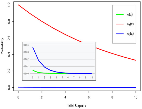
Figure 1. Ruin probability for model of Example 1.

The second IRRM which we present here is generated by exponentially distributed claims and inter occurrence times. We show that we can also derive the upper exponential bounds for ruin probability using Corollaries 3 and 4 again.

Example 2.

Let us consider IRRM generated by constant premium rate $p=1$, a sequence of claims $\{Z_1,Z_2,\dots \}$ having exponential distributions

$$\begin{array}{ccc}\hfill \mathbb{P}(Z_k⩽x)& =& \left(1-{\mathrm{e}}^{-x}\right)1{\mathrm{I}}_{[0,\infty )},k\in \{1,3,5,\dots \},\hfill \\ \hfill \mathbb{P}(Z_k⩽x)& =& \left(1-{\mathrm{e}}^{-x/2}\right)1{\mathrm{I}}_{[0,\infty )},k\in \{2,4,6,\dots \},\hfill \end{array}$$

and a sequence of inter occurrence times $\{{\theta }_1,{\theta }_2,\dots \}$ also having exponential distributions

$$\begin{array}{ccc}\hfill \mathbb{P}({\theta }_k⩽x)& =& \left(1-{\mathrm{e}}^{-x}\right)1{\mathrm{I}}_{[0,\infty )},k\in \{1,3,5,\dots \},\hfill \\ \hfill \mathbb{P}({\theta }_k⩽x)& =& \left(1-{\mathrm{e}}^{-x/3}\right)1{\mathrm{I}}_{[0,\infty )},k\in \{2,4,6,\dots \}.\hfill \end{array}$$

It is obvious that $\mathbb{E}{Z}_k=\mathbb{E}{\theta }_k=1$ for $k\in \{1,3,5,\dots \}$ and $\mathbb{E}{Z}_k=2,\mathbb{E}{\theta }_k=3$ for $k\in \{2,4,6,\dots \}$. Hence, for $n⩾2$, we have

$$\begin{array}{ccc}& & \frac{1}{n}\sum _{k=1}^n(\mathbb{E}{Z}_k-p\mathbb{E}{\theta }_k)⩽-\frac{1}{3},\hfill \end{array}$$

$$\begin{array}{ccc}& & \frac{1}{n}\sum _{k=1}^n\mathbb{E}\left({\theta }_{k}1{\mathrm{I}}_{\{{\theta }_k⩾u\}}\right)\hfill \\ & =& \frac{1}{n}\left(⌊\frac{n+1}{2}⌋{\int }_u^{\infty }y{\mathrm{e}}^{-y}\mathrm{d}y+⌊\frac{n}{2}⌋{\int }_u^{\infty }\frac{y}{3}{\mathrm{e}}^{-y/3}\mathrm{d}y\right)\hfill \\ & =& \frac{1}{n}\left(⌊\frac{n}{2}⌋{\mathrm{e}}^{-u}(u+1)+⌊\frac{n}{2}⌋{\mathrm{e}}^{-u/3}(u+3)\right),\hfill \\ & & \frac{1}{n}\sum _{k=1}^n\left(\mathbb{P}(Z_k-p{\theta }_k⩽0)+\mathbb{E}\left({\mathrm{e}}^{(Z_k-p{\theta }_k)/6}1{\mathrm{I}}_{\{Z_k-p{\theta }_k>0\}}\right)\right)\hfill \\ & =& \frac{1}{n}⌊\frac{n+1}{2}⌋\left(\mathbb{P}(Z_1-{\theta }_1⩽0)+\mathbb{E}\left({\mathrm{e}}^{(Z_1-{\theta }_1)/6}1{\mathrm{I}}_{\{Z_1-{\theta }_1>0\}}\right)\right)\hfill \\ & & +\frac{1}{n}⌊\frac{n}{2}⌋\left(\mathbb{P}(Z_2-{\theta }_2⩽0)+\mathbb{E}\left({\mathrm{e}}^{(Z_2-{\theta }_2)/6}1{\mathrm{I}}_{\{Z_2-{\theta }_2>0\}}\right)\right)\hfill \\ & =& \frac{1}{n}\left(⌊\frac{n+1}{2}⌋\frac{11}{10}+⌊\frac{n}{2}⌋\frac{12}{10}\right)⩽\frac{23}{20}.\hfill \end{array}$$

After some calculations, we obtain that conditions of Corollary 3 hold with the following collection of constants.

$$A=1/3,B=2,C=12,\Delta =11/80,H=1/6,d^{*}=23/20.$$

In addition,

$$\begin{array}{ccc}\hfill D^{*}& =& \mathbb{P}(Z_1-p{\theta }_1⩽0)+\mathbb{E}\left(\left({\mathrm{e}}^{(Z_1-p{\theta }_1)/6}\right)1{\mathrm{I}}_{\{Z_1-p{\theta }_1>0\}}\right)\hfill \\ & =& \mathbb{P}(Z_1-p{\theta }_1⩽0)+\underset{0}{\overset{\infty }{\int }}{\mathrm{e}}^{-5y/6}\left(\underset{0}{\overset{x}{\int }}{\mathrm{e}}^{-7z/6}\mathrm{d}z\right)\mathrm{d}y=\frac{11}{10},\hfill \end{array}$$

and

$$\Delta +\delta H{d}^{*}max\left\{\frac{C^2}{2},\frac{2}{H^2}\right\}-A⩽0,$$

if $\delta ⩽47/3312$. Therefore, we can suppose that $\delta =7/500$.

In such a case, we get from Corollary 3 that

$$\psi \left(x\right)⩽{\psi }_1\left(x\right):=min\left\{1,\frac{11}{10}exp\{-7x/3000\}\right\},x⩾0.$$

It is evident that the obtained estimate has the exponential form but it is quite conservative. The reason for this is the generality of the Corollary 3. The last estimate holds for wide group of IRRMs. In fact, the estimate presented in Corollary 3 is not sensitive to the structure of the model. Fortunately, in the example under consideration, the cumulant generating functions of r.v.s ${\left\{Z_k-p{\theta }_k\right\}}_{k=1}^{\infty }$ have sufficiently simple analytic expressions. Hence we can derive more sharp estimate for the model ruin probability using Corollary 4.

Namely, if $k\in \{1,3,5,\dots \}$ and $h\in [0,1)$, then

$$\mathbb{E}\left({\mathrm{e}}^{h(Z_k-p{\theta }_k)}\right)=\frac{1}{1-h^2}.$$

If $k\in \{2,4,6,\dots \}$ and $h\in [0,1/2)$, then

$$\mathbb{E}\left({\mathrm{e}}^{h(Z_k-p{\theta }_k)}\right)=\frac{1}{(1-2h)(1+3h)}.$$

Consequently,

$$\begin{array}{ccc}\hfill \sum _{k=1}^{n}log\left(\mathbb{E}\left({\mathrm{e}}^{h(Z_k-p{\theta }_k)}\right)\right)& =& ⌊\frac{n+1}{2}⌋log\frac{1}{1-h^2}+⌊\frac{n}{2}⌋log\frac{1}{(1-2h)(1+3h)}\hfill \\ & ⩽& \frac{n+1}{2}log\frac{1}{(1-h^2)(1-2h)(1+3h)}⩽0\hfill \end{array}$$

for all $n\in \mathbb{N}$ if $h\in [0,0.1424)$.

By supposing $h=1/8$ we obtain from Corollary 4 that

$$\psi \left(x\right)⩽{\psi }_2\left(x\right):=exp\{-x/8\}$$

for all initial surplus values $x⩾0$.

Below, in Figure 2, we illustrate the results obtained. In the figure, we can see the values of ruin probability $\psi \left(x\right)$ obtained by the Monte Carlo method, its conservative estimate ${\psi }_1\left(x\right)$ and its sharp estimate ${\psi }_2\left(x\right)$.

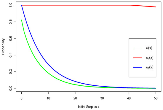
Figure 2. Ruin probability for model of Example 2.

The last our example shows that for particular IRRM a sharper upper bound compared to the standard exponential estimate for ruin probability can be derived. For this we need to apply Corollary 4, because using Corollary 3 we can get only the standard exponential upper estimate, and the model should be generated by random claims ${\left\{Z_k\right\}}_{k=1}^{\infty }$ having finite exponential moments ${\left\{\mathbb{E}{\mathrm{e}}^{h{Z}_k}\right\}}_{k=1}^{\infty }$ for all positive h.

Example 3.

Suppose that IRRM is generated by a premium rate $p=1$, a sequence of degenerated inter occurrence times ${\theta }_k=k,k\in \mathbb{N},$ and a sequence of i.i.d. Poisson random claims $\{Z_1,Z_2,\cdots \}$ such that

$$\mathbb{P}(Z_1=j)=\frac{1}{\mathrm{e}j!},j=0,1,2,\dots$$

In the case under consideration, we have that

$$log\left(\mathbb{E}\left({\mathrm{e}}^{h(Z_k-p{\theta }_k)}\right)\right)=e^h-k-1$$

for all $k\in \mathbb{N}$ and $h⩾0$.

Therefore,

$$\begin{array}{ccc}\hfill \sum _{k=1}^{n}log\left(\mathbb{E}\left({\mathrm{e}}^{h(Z_k-p{\theta }_k)}\right)\right)& =& n({\mathrm{e}}^h-1)-\frac{1+n}{2}n\hfill \\ & ⩽& n({\mathrm{e}}^h-1)-\frac{n^2}{2}\hfill \\ & ⩽& {\left({\mathrm{e}}^h-1\right)}^2/2\hfill \end{array}$$

if $h>0$ and $n\in \mathbb{N}$.

Hence, according to Corollary 4 we get that

$$\psi \left(x\right)⩽exp\left\{-hx+{({\mathrm{e}}^h-1)}^2/2\right\}⩽exp\left\{-hx+\frac{h}{2}{\mathrm{e}}^{2h}\right\}$$

for all positive x and h.

If we choose $h=\frac{1}{2}logx$, by supposing that $x⩾1$, then the last estimate implies that

$$\psi \left(x\right)⩽exp\{-\frac{x}{4}logx\}={\left(\frac{1}{x}\right)}^{x/4},x⩾1.$$

Below, in Figure 3, we illustrate the results obtained. In the figure, red line is the derived upper bound for ruin probability, and green line is the values of $\psi \left(x\right)$ obtained by the Monte Carlo method.

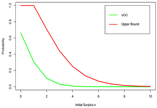
Figure 3. Ruin probability for model of Example 3.

References

- Kiefer, J.; Wolfowitz, J. On the characteristics of the general queuing process with applications to random walk. Ann. Math. Stat. 1956, 27, 147–161. [Google Scholar]
- Sgibnev, M.S. Submultiplicative moments of the supremum of a random walk with negative drift. Stat. Probab. Lett. 1997, 32, 377–383. [Google Scholar] [CrossRef]
- Andrulytė, I.M.; Bernackaitė, E.; Kievinaitė, D.; Šiaulys, J. A Ludberg-type inequality for an inhomogeneous renewal risk model. Mod. Stoch. Theory Appl. 2015, 2, 173–184. [Google Scholar]
- Kievinaitė, D.; Šiaulys, J. Exponential bounds for the tail probability of the supremum of an inhomogeneous random walk. Mod. Stoch. Theory Appl. 2018, 5, 129–143. [Google Scholar] [CrossRef]
- Chernoff, H. A measure of asymptotic efficiency for tests of a hypothesis based on the sum of observations. Ann. Math. Stat. 1952, 23, 493–507. [Google Scholar] [CrossRef]
- Hoeffding, W. Probability inequalities for sums of bounded random variable. J. Am. Stat. Assoc. 1963, 58, 13–30. [Google Scholar]
- Bernstein, S.N. On a modifecation of Chebyshev’s inequality and of the error formula of Laplace. Uchenye Zap. Nauch-Issled. Kaf. Ukr. Sect. Math. 1924, 1, 38–48. (In Russian) [Google Scholar]
- Bernstein, S.N. On certain modifications of Chebyshev’s inequality. Dokl. Akad. Nauk SSSR 1937, 17, 275–277. (In Russian) [Google Scholar]
- Azuma, K. Weighted sum of certain independent random variables. Tohoku Math J. 1967, 19, 357–367. [Google Scholar]
- Bennett, G. Probability inequalities for the sum of independent random variables. J. Am. Stat. Assoc. 1962, 57, 33–45. [Google Scholar] [CrossRef]
- Bentkus, V. An inequality for tail probabilities of martingales with differences bounded from one side. J. Theor. Probab. 2003, 16, 1848–1869. [Google Scholar]
- Fan, X.; Gramma, I.; Liu, Q. Exponential inequalities for martingales with applications. Electron. J. Probab. 2015, 20, 1–22. [Google Scholar] [CrossRef]
- Nagaev, S.T. Large deviations of sums of independent random variables. Ann. Probab. 1979, 7, 745–789. [Google Scholar] [CrossRef]
- Pinelis, I. On normal domination of (super)martingales. Electron. J. Probab. 2006, 11, 1049–1070. [Google Scholar] [CrossRef]
- Pinelis, I. Binimial upper bounds on generalized moments and tail probabilities of (super)martingales with differences bounded from above. IMS Lect. Notes-Monogr. Ser. High Dimentional Probab. 2006, 51, 33–52. [Google Scholar]
- Fisher, R.A. Moments and product moments of sampling distributions. Proc. Lond. Math. Soc. 1929, 30, 199–238. [Google Scholar] [CrossRef]
- Asmussen, S.; Albrecher, H. Ruin Probabilities; World Scientific Publishing: Singapore, 2010. [Google Scholar]
- Embrechts, P.; Klüppelberg, C.; Mikosch, T. Modeling Extremal Events for Insurance and Finance; Springer-Verlag: Berlin/Heidelberg, Germany, 1997. [Google Scholar]
- Embrechts, P.; Veraverbeke, V. Estimates for probability of ruin with special emphasis of the possibility of large claims. Insur. Math. Econ. 1982, 1, 55–72. [Google Scholar] [CrossRef]
- Gerber, H. Martingales in risk theory. Bull. Swiss Asoc. Actuar. 1973, 1973, 205–216. [Google Scholar]
- Mikosch, T. Non-life Insurance Mathematics; Springer-Verlag: Berlin/Heidelberg, Germany, 2009. [Google Scholar]
- Bieliauskienė, E.; Šiaulys, J. Gerber–Shiu function for the discrete inhomogeneous claim case. Int. J. Comput. Math. 2012, 89, 1617–1630. [Google Scholar] [CrossRef]
- Blaževičius, K.; Bieliauskienė, E.; Šiaulys, J. Finite-time ruin probability in the inhomogeneous claim case. Lith. Math. J. 2010, 50, 260–270. [Google Scholar] [CrossRef]
- Castañer, A.; Claramunt, M.M.; Gathy, M.; Lefèvre, C.; Mármol, M. Ruin problems for a discrete time risk model with non-homogeneous conditions. Scand. Actuar. J. 2013, 2013, 83–102. [Google Scholar] [CrossRef]
- Damarackas, J.; Šiaulys, J. Bi-seasonal discrete time risk model. Appl. Math. Comput. 2014, 247, 930–940. [Google Scholar] [CrossRef]
- Grigutis, A.; Šiaulys, J. Ultimate time survival probability in three-risk discrete time risk model. Mathematics 2020, 8, 147. [Google Scholar] [CrossRef]
- Grigutis, A.; Korvel, A.; Šiaulys, J. Ruin probabilities at a discrete-time multi risk model. Inf. Technol. Control 2015, 44, 367–379. [Google Scholar] [CrossRef]
- Grigutis, A.; Korvel, A.; Šiaulys, J. Ruin probability in the three-seasonal discrete-time risk model. Mod. Stoch. Theory Appl. 2015, 2, 421–441. [Google Scholar] [CrossRef][Green Version]
- Navickienė, O.; Sprindys, J.; Šiaulys, J. The Gerber–Shiu discounted penalty function for the bi-seasonal discrete time risk model. Informatica 2018, 29, 733–756. [Google Scholar] [CrossRef]
- Navickienė, O.; Sprindys, J.; Šiaulys, J. Ruin probability for the bi-seasonal discrete time risk model with dependent claims. Mod. Stoch. Theory Appl. 2019, 6, 133–144. [Google Scholar] [CrossRef]
- Răducan, A.M.; Vernic, R.; Zbăganu, G. Recursive calculation of ruin probabilities at or before claim instants for non-identically distributed claims. ASTIN Bull. 2015, 45, 421–443. [Google Scholar] [CrossRef]
- Albrecher, H.; Vatamidu, E. Ruin probability approximations in Sparre-Andersen models with completely monotone claims. Risks 2019, 7, 104. [Google Scholar] [CrossRef]
- Ambagaspitiya, R.S. Ultimate ruin probability in the Sparre-Andersen model with dependent claim sizes and claim occurrence times. Insur. Math. Econ. 2009, 44, 464–472. [Google Scholar] [CrossRef]
- Bareche, A.; Cherfaoui, M. Sensivity of the stability bounds for ruin probabilities to claim distributions. Methodol. Comput. Appl. Probab. 2019, 21, 1259–1281. [Google Scholar] [CrossRef]
- Bernackaitė, E.; Šiaulys, J. The finite-time ruin probability for an inhomogeneous renewal risk model. J. Ind. Manag. Optim. 2017, 13, 207–222. [Google Scholar] [CrossRef][Green Version]
- Bulinskaja, E. Asymptotic analysis and optimization of some insurance models. Appl. Stoch. Model. Bus. Ind. 2018, 34, 762–773. [Google Scholar] [CrossRef]
- Hipp, C. Company value with ruin constraint in Lundberg models. Risks 2018, 6, 73. [Google Scholar] [CrossRef]
- Kizinevič, E.; Šiaulys, J. The exponential estimate of the ultimate ruin probability for the non-homogeneous renewal risk model. Risks 2018, 6, 20. [Google Scholar] [CrossRef]
- Li, S.; Lu, Y.; Sendova, K.P. The expected discounted penalty function: From infinite time to finite time. Scand. Actuar. J. 2019, 2019, 336–354. [Google Scholar] [CrossRef]
- Lefèvre, C.; Loisel, S.; Tamturk, M.; Utev, S. A quantum-type approach to non-life insurance risk modelling. Risks 2018, 6, 99. [Google Scholar] [CrossRef]
- Sun, Z. Upper bounds for ruin probabilities under model uncertainty. Commun. Stat.-Theory Methods 2019, 48, 4511–4527. [Google Scholar] [CrossRef]
- Tang, Q.; Yang, Y. Interplay of insurance and finacial risks in a stochastic environment. Scand. Actuar. J. 2019, 2019, 432–451. [Google Scholar] [CrossRef]
- Shiryaev, A.N. Probability; Springer-Verlag: New York, NY, USA, 1984. [Google Scholar]
- Zhou, Q.; Sakhanenko, A.; Guo, J. Lundberg-type inequalities for non-homogeneous risk models. arXiv 2020, arXiv:2004.11190v2. [Google Scholar]
- Blackwell, D. On an equation of Wald. Ann. Math. Stat. 1946, 17, 84–87. [Google Scholar] [CrossRef]
- Blom, G. A generalization of Wald’s fundamental identity. Ann. Math. Stat. 1949, 20, 439–444. [Google Scholar] [CrossRef]
- Ruben, H. A theorem on the cumulative product of independent random variables. Math. Proc. Camb. Philos. Soc. 1959, 55, 333–337. [Google Scholar] [CrossRef]
- Wald, A. On cumulative sums of random variables. Ann. Math. Stat. 1944, 15, 283–296. [Google Scholar] [CrossRef]
- Wald, A. Differentiation under the expectation sign in the fundamental identity of sequential analysis. Ann. Math. Stat. 1946, 17, 493–497. [Google Scholar] [CrossRef]
- Wolfowitz, J. The efficiency of sequential estimates and Wald’s equation for sequential processes. Ann. Math. Stat. 1947, 18, 215–230. [Google Scholar] [CrossRef]
© 2020 by the authors. Licensee MDPI, Basel, Switzerland. This article is an open access article distributed under the terms and conditions of the Creative Commons Attribution (CC BY) license (http://creativecommons.org/licenses/by/4.0/).