Exploitation of a Productive Asset in the Presence of Strategic Behavior and Pollution Externalities

Abstract

We study the strategic behavior of firms competing in the exploitation of a common-access productive asset, in the presence of pollution externalities. We consider a differential game with two state variables (asset stock and pollution stock), and by using a piecewise-linear approximation of the nonlinear asset growth function, we provide a tractable characterization of the symmetric feedback–Nash equilibrium with asymptotically stable steady state(s). The results show that the firm’s strategy takes three forms depending on the pair of state variables and that different options for the model parameters lead to contrasting outcomes in both the short- and long-run equilibria.

1. Introduction

There is an extensive literature in economics, operations research, game theory, and dynamic optimization dealing with the exploitation of renewable resources (e.g., a fishery or a forest). One main question shared by all parties, namely firms, governments (regulators), and citizens, is how to exploit these resources in a sustainable way. In the vast dynamic games literature, where players (firms and regulators) interact strategically over time, the models have very often focused on the resource itself, without any other considerations. Typically, these models start with a dynamic system describing the evolution of the stock, and next, they characterize the equilibrium strategies under different assumptions related (i) to the information structure (e.g., open-loop, feedback, or closed-loop with or without memory) and (ii) to the players’ behavior (cooperative or noncooperative).

There is ample evidence showing that the evolution of renewable resources depends not only on natural variations and on human intervention (harvesting, deforestation, etc.) but also on the accumulated pollution. An illustrative example is the recent discovery—devastating for biomass—of over 5 trillion pieces of plastic, weighing a total of 250,000 tons, afloat on the Pacific Ocean. More than half of this island of plastic is made of fishing gear, i.e., is the result of resource exploitation [1]. In addition to the adverse effects of accumulated pollution on the resources, the literature documented various direct economic costs borne by firms operating in these industries. For instance, the fishing industry faces costs arising from the need to repair or replace gear that has been damaged or lost because of encounters with abandoned, lost, or otherwise discarded fishing gear (ALDFG) [2,3]. The impacts of ALDFG on fisheries also include hazards to navigation and safety at sea, which increase fuel costs and reduce fishing time, and loss of earnings due to reduced or contaminated catches including ghost fishing [4,5]. It is estimated that the cost of marine debris damage on the fishing industry in 2008 was US$364 million for the 21 Pacific Rim economies [6], and the derelict pot removal program between 2008–2014 in the largest estuary of the United States, the Chesapeake Bay, led to an additional harvest valued at US$21.3 million—a 27% increase above that which would have occurred without removals [7].

Scientists from various disciplines have proposed models to integrate the influence of other (state) variables—e.g., pollution stock, marine environmental quality, and habitat quality—in their analysis (e.g., [8]), omitting, however, the strategic interactions between the various parties involved. In this paper, we consider an oligopoly exploiting a renewable resource (a productive asset) and contribute to the literature by having a more realistic model where strategic behavior and pollution externalities are present. Indeed, strategic thinking has often been ignored in large-scale ecosystem models and in representative-agent frameworks and pollution has been disregarded in games of renewable-resource exploitation.

To represent the habitat’s limited carrying capacity, the rate of growth of the productive asset is typically modeled as a nonlinear, inverted U-shaped function of the asset stock (see, e.g., [9]). The author of [10,11] approximated this nonlinear rate of growth by an inverted-V function, which allowed for tractable characterization of the equilibrium strategies and payoffs. In this work, which is a revised version of [12], we adopt a differential game framework that extends the productive-asset model in [11] by introducing a second state variable, namely pollution stock, while retaining his approximation approach. The game is played by n identical firms competing à la Cournot over an infinite planning horizon. Each player aims to maximize their stream of discounted payoff, taking into account the market structure, the initial size of each stock, and their dynamics. For the present work, we abstract from the effects of pollution on the reproductive capacity of the asset and consider only the direct economic costs of pollution incurred by the firms as negative externality. The problem is technically an infinite horizon linear-quadratic n-player differential game with two state variables and one control variable for each player, which influences the two dynamic processes.

We characterize fully analytically the symmetric feedback–Nash equilibrium, where the firm’s strategy is a piecewise-linear function in the two state variables, for which the shape depends on the position of the game in the state space. Thus, the contribution of this work includes obtaining a closed-form solution in a model with two state variables and a piecewise-linear resource growth function. We show that the state space is divided into three regions, namely scarcity, abundance, and no exploitation. Three equilibrium cases are identified and are shown to depend on the relationship between the asset growth rate, the discount rate, and the pollution decay rate. This equilibrium is sustainable; that is, for any given pair of initial asset–pollution stocks, it converges to a stable steady state with positive exploitation and positive values of state variables. When there are at least two players, the equilibrium includes either one stable or two locally stable steady states; however, when the industry is monopolistic, the optimal solution includes only one stable steady state.

Our work belongs quite naturally to the literature on the exploitation of productive assets and the management of resources under pollution control. Early contributions in this area include [13,14], both of which explored the set of equilibria in a dynamic game framework. The characterization of the equilibrium in [10,11] showed that the firm’s strategy and the value function take piecewise forms, which depends on the asset stock level. There can be a unique or multiple steady states depending on the asset growth rate, and the decision of a single firm to unilaterally decrease its exploitation may result in a decrease in the asset stock. These contributions led to extensive research on various topics related to the strategic exploitation of common access resources that also took into account the nonlinearity of the growth rule. The literature has examined issues such as optimal taxation [15], losses from competition [16], the role of property rights, and convergence to the Cournot equilibrium [17,18]. More recently, [19] showed results on pre-emption, voracity, and exhaustion. The authors of [20] showed that nonlinear feedback strategies are unstable in a dynamic duopoly game with renewable resource exploitation. The effects of mergers were analyzed in [21], the impact of social status concern in these industries were studied in [22], and [23] investigated the incentives in a duopoly by considering a finite planning horizon.

In parallel to this dynamic-games literature on resources, a significant literature has dealt with the strategic behavior of agents under pollution externalities (see the surveys in [24,25]). The pioneering contributions are [26,27], where both noncooperative and cooperative solutions were characterized and contrasted. Many papers have ensued, focusing on issues such as taxation (e.g., [28,29]), sustainability and uncertainty (e.g., [30,31]), international environmental agreements (e.g., [32,33]), and technical change and R&D (e.g., [34]).

Some studies have integrated pollution accumulation in the exploitation of a renewable resource (see, e.g., [35,36,37]). However, these contributions have not accounted for strategic behavior or, when they have, they omitted the feature that the resource growth rate is not linear. In a closely related work to ours, [38] considered a similar model with two state variables, namely biomass stock and pollution stock. They studied a sustainable cooperative agreement in an open-access fishery and characterized the symmetric noncooperative and cooperative solutions. They focused only on an interior solution that includes one part of the solution (which we name the scarcity region). Moreover, they considered the damage of pollution on the resource dynamics together with the damage on welfare, and in the present paper, we study the effect of taking into account the direct economic damage on the firms’ profits. In addition, we characterize the equilibrium for the whole state space and study in detail the boundary cases and the values of parameters that allow for a feedback–Nash equilibrium.

In a nutshell, our paper attempts to integrate within the same framework the exploitation of a productive asset in the presence of pollution externalities and strategic behavior. We approximate the nonlinear growth function by a piecewise linear function, which allows us to have a tractable linear-quadratic dynamic game, for which the equilibria can be characterized analytically.

The rest of the paper is organized as follows: Section 2 introduces the model, Section 3 characterizes the equilibrium and shows its properties, and Section 4 concludes.

2. The Model

We consider an n-player infinite-horizon differential game, with the asset stock S and the pollution stock Z being the two state variables. The model extends the framework in [11] by introducing pollution externalities in the firms’ decision-making problem. At each date $t\in \left[\left.0,+\infty \right)\right.$, n-firms exploit the common-access asset in quantities $q_i(t),i=1,\dots ,n$, and compete à la Cournot. We assume that the exploitation strategy $q_i(t)$ is nonnegative and bounded above, that is, $0\le q_i(t)\le MS(t)$ with the positive constant M sufficiently large (see [14,39] that considered similar constraints). We consider the transformation rate of the asset to the final product to be one-to-one and the unit cost of exploitation to be zero for simplicity. The price p is determined by the linear inverse-demand function given by $p(Q)=a-bQ$, where $Q={\sum }_{i=1}^n{q}_i$ is the total quantity of supply and where $a>0$ and $b>0$.

The growth rate of the productive asset (e.g., a fishery, a forest, etc.) is assumed to be nonlinear in an inverted U–shape in the asset stock. Following the literature, we adopt the following piecewise-linear approximation:

$$f(S)=\left\{\begin{array}{cc}\delta S\hfill & \hfill \mathrm{if}S\le S_y,\\ \delta (S_{max}-S)\hfill & \hfill \mathrm{if}S>S_y,\end{array}\right.$$

(1)

where $\delta >0$ denotes the intrinsic growth rate of the asset and $S_y$ is the level of asset that leads to the so-called maximum sustainable yield ($S_y=\frac{S_{max}}{2}$) with $S_{max}>0$ being the carrying capacity of the habitat. Note that $f(S)=0$ if $S=\left\{0,S_{max}\right\}$, $f(S)>0$ if $S\in \left(0,S_{max}\right)$, and $f(S)<0$ if $S>S_{max}$. Taking into account an asset growth function that includes pollution (i.e., $f(S,Z)$) would allow to capture the negative impacts of pollution on the asset stock. This is considered in [38], where they present the closed-form solutions for noncooperative and cooperative cases for a part of the interior solution. In this work, we refrain from adding pollution and use function $f(S)$ to keep the presentation of results simpler.

Taking into account the firms’ exploitation, the change in the asset stock at date t is governed by the following differential equation:

$$\frac{dS(t)}{dt}=\dot{S}\left(t\right)=f(S(t))-\sum _{i=1}^n{q}_i(t).$$

(2)

The firms’ activities generate emissions as a by-product and add up to the pollution stock, which evolves over time as follows:

$$\frac{dZ(t)}{dt}=\dot{Z}\left(t\right)=\alpha \sum _{i=1}^n{q}_i(t)-kZ(t),$$

(3)

where $\alpha >0$ denotes the amount of emissions resulting from exploiting a unit of asset, and $k>0$ is the pollution decay rate.

Denote by $d\left(Z\right)$ the (symmetric) damage cost of player i. We suppose that this environmental cost is convex increasing in the pollution stock Z and satisfies the property $d\left(0\right)=0$. For tractability, we adopt the quadratic functional form $d(Z)=\frac{\varphi }{2}{Z}^2$, where $\varphi >0$.

Assuming that each player maximizes their discounted stream of profit, the optimization problem of player i is then as follows:

$$\begin{array}{cc}\hfill & \underset{q_i(t)}{max}{\int }_{t=0}^{+\infty }{e}^{-rt}\left(p\left(\sum _{i=1}^n{q}_i(t)\right)q_i(t)-d(Z(t))\right)dt,\hfill \\ \hfill & \mathrm{subject}\mathrm{to}(2),(3),\mathrm{and}0\le q_i(t)\le MS(t),\hfill \\ \hfill & \mathrm{with}S(0)=S_0>0,Z(0)=Z_0\ge 0\mathrm{given}.\hfill \end{array}$$

(4)

where $r>0$ denotes the common discount rate.

3. The Equilibrium

We consider the equilibrium where firms use feedback information in their decision-making. This is a subgame-perfect equilibrium (also called a Markovian Perfect Nash Equilibrium (MPNE)), in which the firm’s strategy is state dependent and strongly time consistent [40,41]. Denote by $V_i(S(t),Z(t))$ the value function of firm i, which is the discounted sum of profits that the firm obtains in the game starting in state $(S(t),Z(t))$. Unless an ambiguity arises, we shall from now on omit the time argument. Introduce the Hamilton–Jacobi–Bellman (HJB) equation associated to firm i’s maximization problem, that is,

$$r{V}_i(S,Z)=\underset{q_i}{max}\left\{p\left(\sum _{i=1}^n{q}_i\right)q_i-d(Z)+\frac{\partial V_i(S,Z)}{\partial S}\left(f(S)-\sum _{i=1}^n{q}_i\right)+\frac{\partial V_i(S,Z)}{\partial Z}\left(\alpha \sum _{i=1}^n{q}_i-kZ\right)\right\},$$

(5)

for $i=\left\{1,..,n\right\}$, where the partial derivative $\partial V_i(S,Z)/\partial S$ represents the shadow price (or value) of the asset stock (also called scarcity rent) and $\partial V(S,Z)/\partial Z$ denotes the shadow value of the pollution stock. Taking into account the nonnegativity restriction on $q_i$ in problem (4), maximizing the right-hand side of (5) yields the following condition:

$$q_i\ge 0;a-b\sum _{i=1}^n{q}_i-b{q}_i\le \frac{\partial V_i(S,Z)}{\partial S}-\alpha \frac{\partial V_i(S,Z)}{\partial Z},$$

(6)

with at least one of the inequalities being equality. The condition (6) must hold together with the terminal condition ${lim}_{t\to +\infty }{e}^{-rt}V(S(t),Z(t))=0$ for every admissible trajectory. The left-hand side of the second inequality in (6) is the marginal revenue of firm i for given quantities of competitors. The right-hand side represents the marginal (opportunity) cost of a unit of exploitation, which comprises the shadow prices of the asset stock and pollution stock. Since we are considering costless exploitation, the opportunity cost consists only of the shadow prices of the state variables. We focus on a symmetric equilibrium in which all firms have the same value function, and they exploit the same quantities ($V_i(S,Z)=V(S,Z)$ and $q_i=q$ for all $i=\left\{1,..,n\right\}$). Consequently, (6) becomes

$$q^{*}(S,Z)=max\left\{0,\frac{1}{b(n+1)}\left(a-\frac{\partial V(S,Z)}{\partial S}+\alpha \frac{\partial V(S,Z)}{\partial Z}\right)\right\},$$

(7)

for $i=\left\{1,..,n\right\}$. Condition (7) results in two possibilities for the equilibrium strategy, that is, $q^{*}(S,Z)>0$ or $q^{*}(S,Z)=0$. There may exist different cases where $q^{*}(S,Z)>0$ depending on the signs of the partial derivatives of the function $V(S,Z)$. We consider the cases in which the asset has a scarcity rent ($\partial V(S,Z)/\partial S>0$) or not ($\partial V(S,Z)/\partial S=0$), and we consider all possible cases for the effect of pollution on the value of the firm; thus, $sign(\partial V(S,Z)/\partial Z)$ is free. By using (7), we write these cases in the following definition:

Definition 1.

The three regions are as follows:

• Scarcity region ($R_S$):$q^{*}(S,Z)>0$ with $\partial V(S,Z)/\partial S>0$:

  $$\begin{array}{cc}\hfill R_S=\left\{(S,Z)|\left(a>\frac{\partial V(S,Z)}{\partial S}-\alpha \frac{\partial V(S,Z)}{\partial Z}\right)and\left(\frac{\partial V(S,Z)}{\partial S}>0\right)\right\}.& \end{array}$$
• Abundance region ($R_A$):$q^{*}(S,Z)>0$ with $\partial V(S,Z)/\partial S=0$:

  $$\begin{array}{cc}\hfill R_A=\left\{(S,Z)|\left(a>-\alpha \frac{\partial V(S,Z)}{\partial Z}\right)and\left(\frac{\partial V(S,Z)}{\partial S}=0\right)\right\}.& \end{array}$$
• No-exploitation region ($R_0$):$q^{*}(S,Z)=0$:

  $$\begin{array}{cc}\hfill R_0=\left\{(S,Z)|a\le \frac{\partial V(S,Z)}{\partial S}-\alpha \frac{\partial V(S,Z)}{\partial Z}\right\}.& \end{array}$$

In region $R_S$, the pair of state variables is such that it is profitable to exploit the asset, and the asset has a scarcity rent. The firms view the level of the asset stock as scarce, and they consider their impact on the asset stock in their strategy. In region $R_A$, the asset stock is too high, so having an additional unit in the stock brings no value to firms. Players consider only the pollution externality as an intertemporal effect of exploitation, and the asset stock does not play a role in their decision. In region $R_0$, the marginal revenue of an initial asset supply (given by the price $P(0)=a$) is lower than its marginal cost, which depends on the shadow prices of the asset stock and pollution stock. Hence, exploitation is not dynamically profitable and the equilibrium strategy is to wait for the asset to replenish and for pollution to decline.

Since the function V is not known, it is not clear beforehand whether any of these three cases exist. To proceed with an analytically tractable characterization, we focus on the strategies that are linear functions of the state variables. Furthermore, we introduce the following assumptions:

Assumption 1.

$$(a)\frac{r\left(1+n^2\right)}{2}<\delta \le r+kand\varphi <{\varphi }_1,(b)r+k<\delta <\frac{k\left(1+n^2\right)}{n^2-1}and\varphi <{\varphi }_2,$$

where the terms ${\varphi }_1$ and ${\varphi }_2$ are given by

$$\begin{array}{cc}\hfill & {\varphi }_1=\frac{b(k+r)\left(2\delta -\left(n^2+1\right)r\right)\left(\delta \left(2k{n}^2+\left(n^2+1\right)r\right)-\left(n^2+1\right)r(k+r)\right)}{2{(\delta \alpha n(n-1))}^2},\hfill \end{array}$$

(8)

$$\begin{array}{cc}\hfill & {\varphi }_2=\frac{bk(k+r)\left(k\left(n^2+1\right)-\delta \left(n^2-1\right)\right)\left(\left(n^2+1\right)(k+r)+\delta \left(n^2-1\right)\right)}{2{(\delta \alpha n(n-1))}^2},\hfill \end{array}$$

(9)

where we have ${\varphi }_2<{\varphi }_1$ for $n>1$ and $r+k<\delta <\frac{k\left(1+n^2\right)}{n^2-1}$.

Assumption 2.

$$\frac{4ab\left(1+n^2\right)(k+r)(k+\delta )}{\delta (\lambda +b(1+n)r)(\lambda +b(1+n)(2\delta -r))}<S_y,$$

(10)

where $\lambda =\sqrt{{\left(b(n+1)(2k+r)\right)}^2+8n^2{\alpha }^{2}b\varphi }$.

The assumptions above require the intrinsic growth rate of the asset ($\delta$) to be sufficiently high (which is the same condition required in [11]) but also bounded from above with a threshold that depends on the pollution decay rate (k) and the number of firms (n). Another restriction is imposed on the marginal damage parameter $\varphi$, which is required to be sufficiently low. For too high values of $\delta$, the condition is revised to be more strict for the parameter $\varphi$. We will discuss the roles of these restrictions in more detail in Section 3.1, where we study the properties of the equilibrium. In the following theorem, we characterize the symmetric equilibrium:

Theorem 1.

Suppose that Assumptions 1 and 2 are satisfied.

(a) 

Equilibrium strategies:

The strategy profile $\left\{q_1(t),..,q_n(t)\right\}$$=\left\{q^{*}(S(t),Z(t)),..,q^{*}(S(t),Z(t))\right\}$ for $t\in \left[\left.0,+\infty \right)\right.$ where

$$q^{*}(S,Z)=\left\{\begin{array}{ccc}(a+c_0+c_{S}S+c_{Z}Z)/b(n+1)\hfill & \hfill if& (S,Z)\in R_S,\hfill \\ (a+{\overline{c}}_0+{\overline{c}}_{Z}Z)/b(n+1)\hfill & \hfill if& (S,Z)\in R_A,\hfill \\ 0\hfill & \hfill if& (S,Z)\in R_0,\hfill \end{array}\right.$$

(11)

constitutes a symmetric feedback–Nash equilibrium.

The terms $\left\{c_S,c_Z,c_0\right\}$ and $\left\{{\overline{c}}_S,{\overline{c}}_Z,{\overline{c}}_0\right\}$, which depend on the exogenous model parameters, are written as follows:

$$\begin{array}{cc}\hfill c_S& =\frac{(n+1)}{4n^2}\frac{(2\delta -r)}{(\delta +k)}\left(\lambda +b(n+1)(2\delta -r)\right),\hfill \end{array}$$

(12)

$$\begin{array}{cc}\hfill c_Z& =\frac{(n+1)}{4n^2\alpha }\frac{(\delta -r-k)}{(\delta +k)}\left(\lambda -b(n+1)(2k+r)\right),\hfill \end{array}$$

(13)

$$\begin{array}{cc}\hfill c_0& =\frac{a\left(n^2+1\right)(c_S(k+r)+\alpha c_Z(\delta -r))}{b{(n+1)}^2(k+r)(\delta -r)-2n^2(c_S(k+r)+\alpha c_Z(\delta -r))},\hfill \end{array}$$

(14)

and

$$\begin{array}{cc}\hfill {\overline{c}}_S& =0,\hfill \end{array}$$

(15)

$$\begin{array}{cc}\hfill {\overline{c}}_Z& =-\frac{(n+1)}{4n^2\alpha }\left(\lambda -b(n+1)(2k+r)\right),\hfill \end{array}$$

(16)

$$\begin{array}{cc}\hfill {\overline{c}}_0& =\frac{a\left(n^2+1\right)\alpha {\overline{c}}_Z}{b{(n+1)}^2(k+r)-2n^2\alpha {\overline{c}}_Z},\hfill \end{array}$$

(17)

where the term λ is given by

$$\lambda =\sqrt{{\left(b(n+1)(2k+r)\right)}^2+8n^2{\alpha }^{2}b\varphi }.$$

(18)

The regions $\left\{R_S,R_A,R_0\right\}$ are written as follows:

$$\begin{array}{cc}\hfill R_S=& \left\{(S,Z)|\left(S>-\frac{a+c_0}{c_S}-\frac{c_Z}{c_S}Z\right)\right.\hfill \end{array}$$

$$\begin{array}{cc}\hfill & \left.and\left(S<\frac{(2\delta -r)}{(k+r-\delta )}\frac{c_Z}{c_S}Z-\frac{(2\delta -r)}{(\delta -r)}\frac{\left(a\left(1+n^2\right)+2n^2{c}_0\right)}{2n^2{c}_S}\right)\right\},\hfill \end{array}$$

(19)

$$\begin{array}{cc}\hfill R_A=& \left\{(S,Z)|\left(Z<-\frac{a+{\overline{c}}_0}{{\overline{c}}_Z}\right)\right.\hfill \end{array}$$

$$\begin{array}{cc}\hfill & \left.\mathrm{and}\left(S\ge \frac{(2\delta -r)}{(k+r-\delta )}\frac{c_Z}{c_S}Z-\frac{(2\delta -r)}{c_S}\frac{\left(a\left(1+n^2\right)+2n^2{c}_0\right)}{2n^2(\delta -r)}\right)\right\},\hfill \end{array}$$

(20)

$$\begin{array}{cc}\hfill R_0=& \left\{(S,Z)|\left(S\le -\frac{a+c_0}{c_S}-\frac{c_Z}{c_S}Z\right)\mathrm{or}\left(Z\ge -\frac{a+{\overline{c}}_0}{{\overline{c}}_Z}\right)\right\}.\hfill \end{array}$$

(21)

(b) 

Value functions:

The discounted sum of profits obtained by each firm is given by the following value function:

$$V_i(S,Z)=V(S,Z)=\left\{\begin{array}{ccc}W(S,Z)\hfill & \hfill if& (S,Z)\in R_S,\hfill \\ \overline{V}(Z)\hfill & \hfill if& (S,Z)\in R_A,\hfill \\ V_0(S,Z)\hfill & \hfill if& (S,Z)\in R_0,\hfill \end{array}\right.$$

(22)

for $i=\left\{1,..,n\right\}$, which is continuously differentiable $\forall (S,Z)\in {\mathbb{R}}_{+}^2$.

The function $W(S,Z)$ is written as follows:

$$W(S,Z)=A+\frac{B}{2}{S}^2+CS+\frac{D}{2}{Z}^2+EZ+FSZ,$$

(23)

where

$$\begin{array}{cccc}\hfill & A=\frac{(a+c_0)\left(a+n^2{c}_0\right)}{b{(n+1)}^{2}r},\hfill & \hfill B& =\frac{2n^2{c}_S^2}{b{(n+1)}^2(r-2\delta )},\hfill \end{array}$$

(24)

$$\begin{array}{cccc}\hfill & C=\frac{c_S\left(a(n^2+1)+2n^2{c}_0\right)}{b{(n+1)}^2(r-\delta )},\hfill & \hfill D& =\frac{2n^2{c}_Z^2-b{(n+1)}^2\varphi }{b{(n+1)}^2(2k+r)},\hfill \end{array}$$

(25)

$$\begin{array}{cccc}\hfill & E=\frac{c_Z\left(a(n^2+1)+2n^2{c}_0\right)}{b{(n+1)}^2(k+r)},\hfill & \hfill F& =\frac{2n^2{c}_Z{c}_S}{b{(n+1)}^2(k+r-\delta )}.\hfill \end{array}$$

(26)

The function $\overline{V}(Z)$ is written as follows:

$$\overline{V}(Z)=\overline{A}+\frac{\overline{D}}{2}{Z}^2+\overline{E}Z,$$

(27)

where

$$\overline{A}=\frac{(a+{\overline{c}}_0)\left(a+n^2{\overline{c}}_0\right)}{b{(n+1)}^{2}r},\overline{D}=\frac{{\overline{c}}_Z}{\alpha },\overline{E}=\frac{{\overline{c}}_0}{\alpha }.$$

(28)

The function $V_0(S,Z)$ is written as follows:

$$V_0(S,Z)={\left(\frac{Z}{\widehat{Z}(S,Z)}\right)}^{-\frac{r}{k}}\mathsf{\Theta }\left(S{\left(\frac{Z}{\widehat{Z}(S,Z)}\right)}^{\frac{\delta }{k}},\widehat{Z}(S,Z)\right)-\frac{\varphi Z^2}{2(2k+r)}\left(1-{\left(\frac{Z}{\widehat{Z}(S,Z)}\right)}^{-\frac{2k+r}{k}}\right),$$

(29)

with

$$\mathsf{\Theta }(S,Z)=\left\{\begin{array}{ccc}W(S,Z)\hfill & \hfill if& (S,Z)\in R_0^W,\hfill \\ \overline{V}(Z)\hfill & \hfill if& (S,Z)\in R_0^{\overline{V}},\hfill \end{array}\right.$$

(30)

and the function $\widehat{Z}(S,Z)$ is defined implicitly by the following system of equations:

$$\begin{array}{c}\hfill \widehat{S}(S,Z)=S{\left(\frac{Z}{\widehat{Z}(S,Z)}\right)}^{\frac{\delta }{k}},\widehat{Z}(S,Z)=-\frac{c_S}{c_Z}\widehat{S}(S,Z)-\frac{a+c_0}{c_Z}.\end{array}$$

(31)

The partitions of region $R_0$, denoted by $R_0^W$ and $R_0^{\overline{V}}$ are written as follows:

$$\begin{array}{cc}\hfill & R_0^W=\left\{(S,Z)\in R_0|Z<Z_3\mathrm{or}{Z}_3\le Z<\mathsf{\Psi }(S)\right\},\hfill \end{array}$$

(32)

$$\begin{array}{cc}\hfill & R_0^{\overline{V}}=\left\{(S,Z)\in R_0|Z\ge Z_3\mathrm{and}Z\ge \mathsf{\Psi }(S)\right\},\hfill \end{array}$$

(33)

where the curve $Z=\mathsf{\Psi }(S)$ denotes the boundary between $R_0^W$ and $R_0^{\overline{V}}$ given by

$$\mathsf{\Psi }(S)=Z_3{\left(\frac{S_3}{S}\right)}^{\frac{k}{\delta }},$$

(34)

with the constants $S_3$ and $Z_3$ given as follows:

$$\begin{array}{cc}\hfill S_3& =\frac{2a\left(2bk\left(n^2+1\right)(k+r)-b\delta \left(n^2-1\right)r-\delta \lambda (n-1)\right)}{\delta (b(n+1)r+\lambda )(\lambda +b(n+1)(2\delta -r))},\hfill \end{array}$$

(35)

$$\begin{array}{cc}\hfill Z_3& =\frac{2a\alpha \left(b\left(2k\left(n^2+1\right)+r\left(3n^2+1\right)\right)+\lambda (n-1)\right)}{(\lambda +b(n+1)r)(\lambda -b(n+1)(2k+r))}.\hfill \end{array}$$

(36)

Proof. 

The long proof is built throughout the paper, and the details are provided in Appendix A, which has several subsections. The road map to complete the proof of the theorem is as follows:

• In Appendix A.1, we state some preliminaries and introduce the methodological approach.
• In Appendix A.2, we study the case $q^{*}(S,Z)>0$. By guessing a piecewise-quadratic form for the value function and by applying the undetermined coefficient method, we obtain the functions $W(S,Z)$ and $\overline{V}(Z)$ and the solutions associated with their coefficients. Then, we analyze the boundary cases and their positions in $(S,Z)$.
• Lemma A1 in Appendix A.2.1 shows that, under Assumptions 1 and 2, the function $W(S,Z)$ satisfies the HJB equation $\forall (S,Z)\in R_S$ and that strategy profile $q_i=q^{*}\forall i$ satisfies (7) with $q^{*}(S,Z)>0$ and $\partial V(S,Z)/\partial S>0$.
• Lemma A2 in Appendix A.2.2 shows that, under Assumptions 1 and 2, the function $V(S,Z)=\left\{W(S,Z)\mathrm{if}(S,Z)\in R_S,\right.$ $\left.\overline{V}(Z)\mathrm{if}(S,Z)\in R_A\right\}$ is continuously differentiable in S and Z and satisfies the HJB equation $\forall (S,Z)\in R_S\cup R_A$. The strategy profile $q_i=q^{*},\forall i$ satisfies (7) with $q^{*}(S,Z)>0$ and $\partial V(S,Z)/\partial S\ge 0$.
• Appendix A.3 looks at the case $q^{*}=0$. Lemma A3 obtains the function $V_0(S,Z)$ and shows that it is continuously differentiable in S and $Z,$ $\forall (S,Z)\in R_0$, and on the boundary cases of $R_0$.
• Combining these results, we conclude that the piecewise function $V(S,Z)$ given in (22) satisfies HJB Equation (5) and that the strategy profile $q_i=q^{*},\forall i$ satisfies the condition in (7) $\forall (S,Z)\in {\mathbb{R}}_{+}^2$ and constitutes a feedback–Nash equilibrium.

 □

Theorem 1 characterizes the symmetric equilibrium strategy of firms for any given pair $(S,Z)$. The strategy $q^{*}(S,Z)$ is a piecewise-linear function in S and Z with coefficients ($c_0,c_S,c_Z$) and (${\overline{c}}_0,{\overline{c}}_Z$) that correspond to the coefficients of the marginal cost function given in (6) (see (A7) in Appendix A.2 in the Appendix A).

For further analysis, we define the boundary lines between the regions as follows:

Definition 2.

Let $Z=Z_i^j(S)$ denote the boundary line in the $(S,Z)$ plane between the regions $R_i$ and $R_j$ as function of S. We have

(i) 

The boundary line between $R_S$ and $R_0$:

$$Z=Z_0^S(S)=-\frac{c_S}{c_Z}S-\frac{a+c_0}{c_Z}.$$

(37)

(ii) 

The boundary line between $R_S$ and $R_A$:

$$Z=Z_S^A(S)=\frac{(k+r-\delta )}{(2\delta -r)}\frac{c_S}{c_Z}S+\frac{(k+r-\delta )\left(a\left(1+n^2\right)+2n^2{c}_0\right)}{2n^2(\delta -r)c_Z}.$$

(38)

(iii) 

The boundary line between $R_A$ and $R_0$:

$$Z=Z_0^A=-\frac{a+{\overline{c}}_0}{{\overline{c}}_Z}.$$

(39)

We now proceed with studying the general properties of the equilibrium in the next subsection.

3.1. The Properties of the Equilibrium

We briefly explain the methods used for obtaining the equilibrium strategies and then investigate their properties. Using a linear-quadratic model with the piecewise-linear approximation of the asset growth function enables us to guess the form of the value function as a polynomial of degree 2 in S and Z within an interior solution. We obtain the six-dimensional equation system associated with the coefficients of $W(S,Z)$ and then reduce it into a system of two equations in ($c_S,c_Z$) given in (A5) and (A6). This system yields four solutions: two include $\partial W(S,Z)/\partial S\ne 0$ and the other two include $\partial W(S,Z)/\partial S=0$. Among all solutions, only one pair makes it possible to characterize a feedback–Nash equilibrium with a stable steady state.

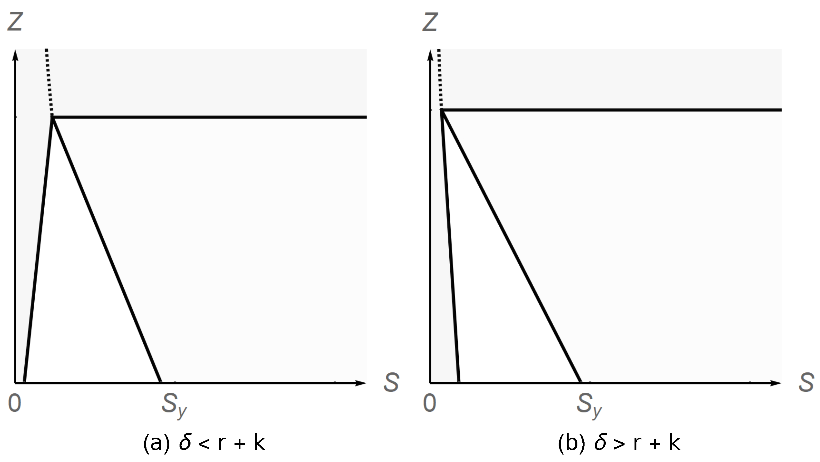
We use the solutions for the strategies and the value function to derive the analytical formulation of the case $R_S$, which is given in (19). We obtain the linear functions associated with its boundary cases, where $q^{*}(S,Z)=0$ and $\partial W(S,Z)/\partial S=0$, and then study their positions in $(S,Z)$ by analyzing the signs of ($c_S,c_Z$) given in Equations (12) and (13), which result in three cases that differ in the relationship among the dynamic model parameters, i.e., $sign(\delta -r-k)$. In all cases, $c_S>0$ and ${\overline{c}}_Z<0$, but the sign of $c_Z$ differs, i.e., $sign(c_Z)=sign(\delta -r-k)$. Using these results, for $\delta >r/2$, we write the following cases:

$$\begin{array}{cc}\hfill \mathrm{Case}1:& \delta <r+k:c_S>0,c_Z<0,{\overline{c}}_Z<0,\hfill \\ \hfill \mathrm{Case}2:& \delta =r+k:c_S>0,c_Z=0,{\overline{c}}_Z<0,\hfill \\ \hfill \mathrm{Case}3:& \delta >r+k:c_S>0,c_Z>0,{\overline{c}}_Z<0.\hfill \end{array}$$

Since $c_Z$ is the coefficient associated with the level of pollution in the equilibrium strategy in region $R_S$, this difference leads to contrasting results in the equilibrium responses to pollution in $R_S$, which will be discussed in detail below.

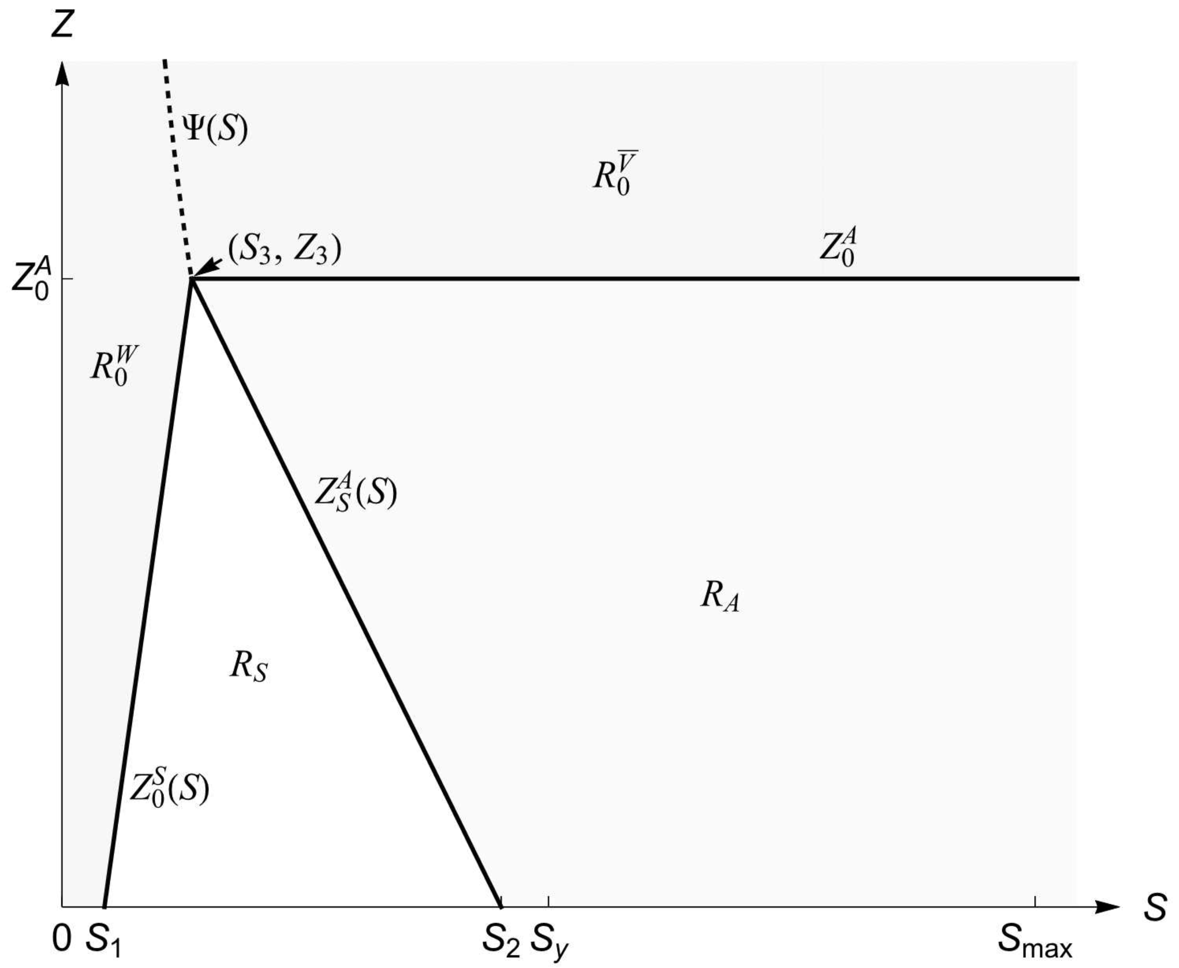
We analyze the properties of the equilibrium by using the diagram in Figure 1, which shows the shapes and positions of the regions given in Definition 1 in the $(S,Z)$ plane.

Figure 1. Illustration of the regions and their boundaries in $(S,Z)$.

(i)

There are four regions: the value function takes a different form in each region.

(ii)

$q^{*}>0$ in $R_S\cup R_A$, and $q^{*}=0$ in $R_0^W\cup R_0^{\overline{V}}$.

(iii)

$\partial V/\partial S>0$ in $R_S\cup R_0^W$, and $\partial V/\partial S=0$ in $R_A\cup R_0^{\overline{V}}$.

(iv)

The boundary case $Z=Z_0^S(S)$ given in (37) denotes the threshold where $q^{*}=0$ and $\partial W/\partial S>0$, beyond which the firms voluntarily cease exploitation and wait for the asset to replenish and pollution to decline. The sign of its slope depends on $sign(r+k-\delta )$.

(v)

The boundary case $Z=Z_S^A(S)$ given in (38) denotes the threshold where $q^{*}>0$ and $\partial W/\partial S=0$. It decreases in S in all cases.

(vi)

The boundary $Z=Z_0^A$ given in (39), which is a positive constant, denotes the threshold level of pollution, where $q^{*}=0$ and $\partial V/\partial S=0$. The firms refrain from any exploitation if the level of pollution is above this threshold.

(vii)

The boundary cases of $R_S$ intersect with the $Z=0$ axis at points $(S_1,0)$ and $(S_2,0)$, and their intersection point is denoted by $(S_3,Z_3)$, where the closed-form solutions of $S_1$, $S_2$, and $(S_3,Z_3)$ are given in (A9), (A10), (35), and (36). When Assumptions 1 and 2 are satisfied, the ordering of these points is given as follows: $0<S_1<S_2<S_y$ and $S_3>0$, $Z_3>0$.

The qualitative properties of equilibrium in region $R_A$ remain the same for all values of parameters that satisfy Assumptions 1 and 2. This is because the firm’s strategy and the value function in this region do not depend on the intrinsic growth rate $(\delta )$. Within this region, the equilibrium behavior is that of the dynamic oligopoly with pollution externalities, where higher pollution induces the firms to exploit less of the asset ($\partial q^{*}/\partial Z<0$). Since the slope of the boundary $d{Z}_S^A(S)/dS<0$ in all cases, for a fixed point on this boundary, $\partial V/\partial S>0$ for lower levels of pollution and $\partial V/\partial S=0$ if pollution is high.

By contrast, the behavior in region $R_S$ differs depending on $sign(\delta -r-k)$. In the following, we show the properties of the equilibrium strategies in each case:

Case 1: 

$\delta <r+k$, $c_S>0$ and $c_Z<0$ (Figure 1 and Figure 2a): The equilibrium level of exploitation is faster if the asset stock is larger ($\partial q^{*}/\partial S>0$), and it is slower if the level of pollution is higher ($\partial q^{*}/\partial Z<0$). Since $d{Z}_0^S(S)/dS>0$, for a fixed pair of state variables on this threshold, firms will exploit the resource if pollution is sufficiently low but will not exploit if pollution is too high.

Figure 2. Two cases of region positioning under Assumptions 1 and 2.

Case 2: 

$\delta =r+k$, $c_S>0$ and $c_Z=0$: The firm’s strategy includes only the asset stock and is independent of the level of pollution. The boundary case where $q^{*}=0$ and $\partial W/\partial S>0$ becomes a constant $S=S_1$.

Case 3: 

$\delta >r+k$, $c_S>0$ and $c_Z>0$ (Figure 2b): In this case, the slope of the threshold $Z=Z_0^S(S)$ becomes negative. Firms exploit the asset faster if the level of pollution is higher ($\partial q^{*}/\partial Z>0$). Since $d{Z}_0^S(S)/dS<0$, for a fixed a point on this threshold, firms exploit the asset if the level of pollution is high and do not exploit it if pollution is low. The opportunity cost of exploitation given in (6) decreases in pollution.

The results presented above highlight the differences in equilibrium behavior among the three cases. For a relatively slow growing asset, the response to pollution is to decrease exploitation; however, if the asset growth rate is sufficiently large, the equilibrium response to pollution is reversed, i.e., to exploit more under higher pollution.

Since we make an extension of [11], it will be useful to compare and contrast our results. Naturally, our solutions share many similarities with [11]. The three regions and the piecewise-linear strategies we obtain are also found in [11], where they depend only on the level of asset stock. This is indeed the consequence of considering a piecewise-linear growth function. Moreover, the solution we present is equivalent to the one given in [11] in the limit case, where the damage function parameter $\varphi \to 0$ (see Remark A1 in Appendix A.2 in the Appendix A). Furthermore, as the damage cost parameter $\varphi$ increases, the equilibrium behavior is more affected by the level of pollution. Our results show that, if the pollution level is too high, the firms do not exploit the asset for any given level of asset stock. Also, for a given set of other parameters, above a level of $\varphi$ given in Assumption 1 ($\varphi >{\varphi }_1$ or $\varphi >{\varphi }_2$ depending on $\delta$, k, and r), we cannot characterize a feedback–Nash equilibrium for the whole state space. Last but not least, the different types of equilibrium responses in cases 1 to 3 appear due to the presence of pollution in the problem.

As mentioned above, when firms do not have information on the pollution externality or when they do not take it into account in their decision-making ($\varphi \to 0$), the equilibrium behavior is as given in [11]. One question is whether the firms benefit from taking into account the damage cost ($d(Z)$) in their profits. When there are direct economic costs due to pollution but the firm disregards it, then the discounted sum of profits the firm obtains will be lower. We elaborate on this by discussing the two following cases: one firm chooses another strategy while all other firms stick with the feedback–Nash strategy with d(Z) in their profit function, and all firms disregard the damage in their profit. For the first case, in which all other firms choose the feedback–Nash strategy ($q^{*}$ given in Equation (11)), one firm deviating and choosing another strategy (denote by $\tilde{q}$ with $\tilde{q}\ne q^{*}$) would yield a lower value, which is immediate because the equilibrium we characterize is subgame-perfect (i.e., $V_i(q_i^{*},q_{-i}^{*})\ge V_i({\tilde{q}}_i,q_{-i}^{*})$, where $q_{-i}^{*}$ denotes all other firms’ strategy except firm i). For the second case, let $q^{\prime }$ denote the symmetric equilibrium strategy in the game without pollution, which is given in [11]. When all firms disregard the damage in their profit and all choose the strategy $q^{\prime }$, one firm can deviate and make larger profits by taking into account $d(Z)$ since $q^{\prime }$ is not maximizer of the problem with $d(Z)$, thus it would not be an equilibrium. For these reasons, it is beneficial for firms to take into account the costs arising from accumulated pollution in their decision-making process.

We can now discuss the roles that Assumptions 1 and 2 play on the characterization of the equilibrium. The first part of Assumption 1, which refers to the case $\delta <r+k$, ensures that the asset quantity $S_1>0$. In addition, having the slope of no-exploitation boundary increasing (see Figure 2a) leads to the result that the equilibrium behavior is not to exploit the asset for too small values of asset stock. In the second part of Assumption 1 ($\delta >r+k$), ensuring $S_1>0$ is not sufficient to characterize a feedback–Nash equilibrium. The reason is that the slope of no-exploitation boundary decreases (see Figure 2b), and if $S_3<0,$ then there may exist equilibrium trajectories leading to asset exhaustion. Hence, we modify the condition to ensure $S_3>0$. Then, in both cases, Assumption 1 guarantees that the equilibrium behavior around the asset level $S=0$ is not to exploit the asset, which renders the asset growth to be positive ($\dot{S}>0$) in the neighborhood of the $S=0$ axis for all levels of pollution, and thus, the asset exhaustion never occurs in the equilibrium. Furthermore, Assumption 2 is to ensure that the value function is continuously differentiable for all $(S,Z)$, particularly for $S=S_y=S_{max}/2$, where the asset growth function in (2) is not continuously differentiable. Also note that, for a given parameter calibration that satisfies Assumption 1, the carrying capacity ($S_{max}$) can be set such that Assumption 2 is satisfied as well.

Lastly, we turn to the case where the equilibrium strategy is to not exploit the asset. To characterize the value function in region $R_0$ given in (21), we use the fact that, in this region, $q_i=0$ for all $i\in \left\{1,..,n\right\}$; thus, the asset stock grows at rate $\delta$ and the pollution stock declines at rate k without an intervention. At a certain date $\widehat{t}$, depending on the initial state $(S(0),Z(0))$, the pair $(S(t),Z(t))$ reaches either one of the boundary cases where firms begin exploitation. The value of the game starting at a point in $R_0$ depends on this boundary point associated with itself, which can be computed. The following steps are taken in Appendix A.3:

(i) 

We define an implicit function denoted by $(\widehat{S}(S,Z),\widehat{Z}(S,Z))$ written in the system of equations in (31), which yields the point (and the date) at which the firms launch their exploitation for $(S,Z)\in R_0$.

(ii) 

Using this function, we obtain the curve denoted by $Z=\mathsf{\Psi }(S)$ given in (34) associated with the intersection point of the three regions $(S_3,Z_3)$ where $W(S_3,Z_3)=\overline{V}(Z_3)$.

(iii) 

This curve enables us to partition region $R_0$ into two parts, denoted by $R_0^W$ and $R_0^{\overline{V}}$ given in (32) and (33), such that the boundary for launching exploitation is known for a given $(S,Z)\in R_0$.

Having obtained the boundary point associated with all points in $(S,Z)\in R_0$, in Lemma A3, we find $V_0(S,Z)$ that satisfies the HJB equation with $q_i^{*}=0,\forall i$ and show its continuity. The function $(\widehat{S}(.),\widehat{Z}(.))$ does not have an analytical solution for $(S,Z)\in R_0^W$, except in special cases $(\delta =k)$ and $(\delta =r+k)$ (see Remark A2 in Appendix A.3 in the Appendix A); nevertheless the characterization of $V_0(S,Z)$ remains tractable. For any other parameter setting, this function has to be computed numerically in order to obtain the value of a point in $R_0^W$. In the other partition, $R_0^{\overline{V}}$, the value function has an analytical form.

3.2. The Equilibrium Dynamics, Steady States, and Stability

In order to analyze the stable steady states of the equilibrium, we derive the set of points such that $\dot{S}(t)=0$ and $\dot{Z}(t)=0$, respectively. Then, we obtain the steady states and study their stability by using the methods provided in [42]. The results are shown in the following theorem:

Theorem 2.

Under Assumptions 1 and 2, the steady state(s) may be single or multiple depending on the parameters.

(i) 

The steady state in region $R_S$ is denoted by ${\xi }_S=(s_S^{\infty },z_S^{\infty })$ and written as follows:

$$\begin{array}{cc}\hfill s_S^{\infty }& =\frac{kn\left(a+c_0\right)}{b\delta k(n+1)-n\left(\alpha \delta c_Z+k{c}_S\right)},\hfill \\ \hfill & =\frac{2ak\left(-b\delta \left(2k\left(n^2+1\right)+\left(n^2+3\right)r\right)+2b\left(n^2+1\right)r(k+r)+\delta \lambda (n-1)\right)}{\delta (b(n+1)r+\lambda )\left(b\delta (2k(n-1)+r(n+1))-b(n+1)r^2-\lambda (\delta -r)\right)},\hfill \end{array}$$

(40)

$$\begin{array}{cc}\hfill z_S^{\infty }& =-\frac{\alpha \delta n\left(a+c_0\right)}{n\left(\alpha \delta c_Z+k{c}_S\right)-b\delta k(n+1)},\hfill \\ \hfill & =\frac{2a\alpha \left(b\delta \left(2k\left(n^2+1\right)+\left(n^2+3\right)r\right)-2b\left(n^2+1\right)r(k+r)-\delta \lambda (n-1)\right)}{(b(n+1)r+\lambda )\left(-b\delta (2k(n-1)+r(n+1))+b(n+1)r^2+\lambda (\delta -r)\right)}.\hfill \end{array}$$

(41)

The steady state ${\xi }_S$ always exists, and it is asymptotically stable for $n\ge 2$.

(ii) 

The steady states in region $R_A$ are denoted by ${\xi }_{A1}=(s_{A1}^{\infty },z_{A1}^{\infty })$ and ${\xi }_{A2}=(s_{A2}^{\infty },z_{A2}^{\infty })$ and written as follows:

$$\begin{array}{cc}\hfill s_{A1}^{\infty }& =\frac{kn(a+{\overline{c}}_0)}{\delta (bk(n+1)-n\alpha {\overline{c}}_Z)},\hfill \\ \hfill & =\frac{2ak\left(b\left(2k\left(n^2+1\right)+3n^{2}r+r\right)+\lambda (n-1)\right)}{\delta (b(n+1)r+\lambda )(2bk(n-1)-b(n+1)r+\lambda )},\hfill \end{array}$$

(42)

$$\begin{array}{cc}\hfill s_{A2}^{\infty }& =S_{max}-\frac{kn(a+{\overline{c}}_0)}{\delta (bk(n+1)-n\alpha {\overline{c}}_Z)},\hfill \\ \hfill & =S_{max}-\frac{2ak\left(b\left(2k\left(n^2+1\right)+3n^{2}r+r\right)+\lambda (n-1)\right)}{\delta (b(n+1)r+\lambda )(2bk(n-1)-b(n+1)r+\lambda )},\hfill \end{array}$$

(43)

$$\begin{array}{cc}\hfill z_{A1}^{\infty }=z_{A2}^{\infty }& ={\stackrel{0}{Z}}_A=\frac{\alpha n\left(a+{\overline{c}}_0\right)}{bk(n+1)-\alpha n{\overline{c}}_Z},\hfill \\ \hfill & =\frac{2a\alpha \left(b\left(2k\left(n^2+1\right)+\left(3n^2+1\right)r\right)+\lambda (n-1)\right)}{(b(n+1)r+\lambda )(b(2k(n-1)-(n+1)r)+\lambda )},\hfill \end{array}$$

(44)

The existence of steady states ${\xi }_{A1}$ and ${\xi }_{A2}$ depends on the following condition:

$$\frac{S_{max}}{2}\frac{b\delta (n+1)}{n{\overline{c}}_Z}-\frac{a+{\overline{c}}_0}{{\overline{c}}_Z}<\frac{\alpha n\left(a+{\overline{c}}_0\right)}{bk(n+1)-\alpha n{\overline{c}}_Z}.$$

(45)

• If (45) is true, then the point ${\xi }_{A1}$ is unstable, whereas ${\xi }_{A2}$ is stable. In that case, there are two locally asymptotically stable steady states $({\xi }_S,{\xi }_{A2})$, and the equilibrium to which a game converges depends on its initial state $(S(0),Z(0))$.
• If (45) is not true, then ${\xi }_S$ is the unique steady state which is asymptotically stable.

Proof. 

See Appendix B. □

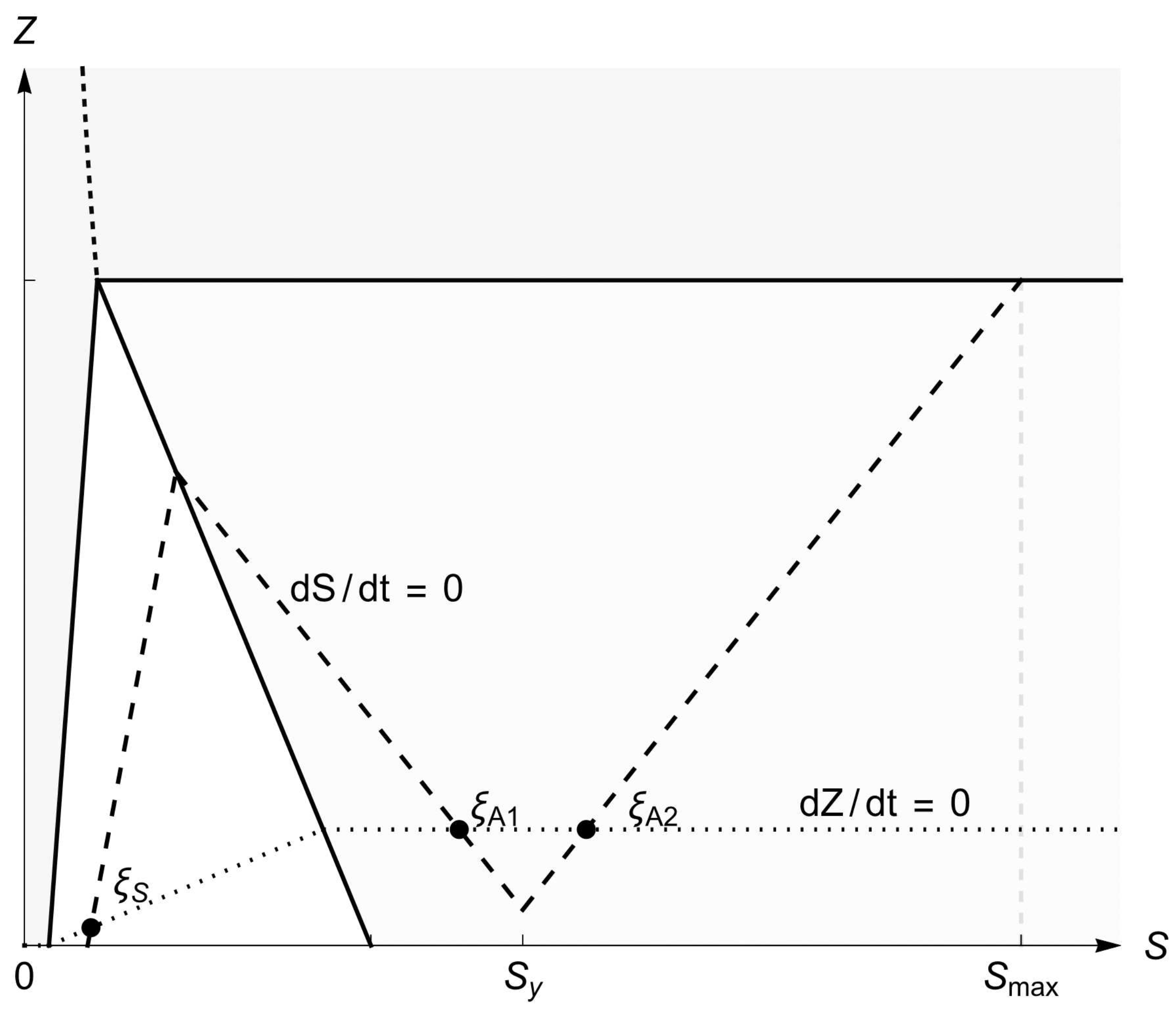
Figure 3 illustrates these results for a case in which multiple steady states exist, which also shows the positions of the loci $\dot{S}=0$ and $\dot{Z}=0$.

Figure 3. Sample of the case with multiple steady states.

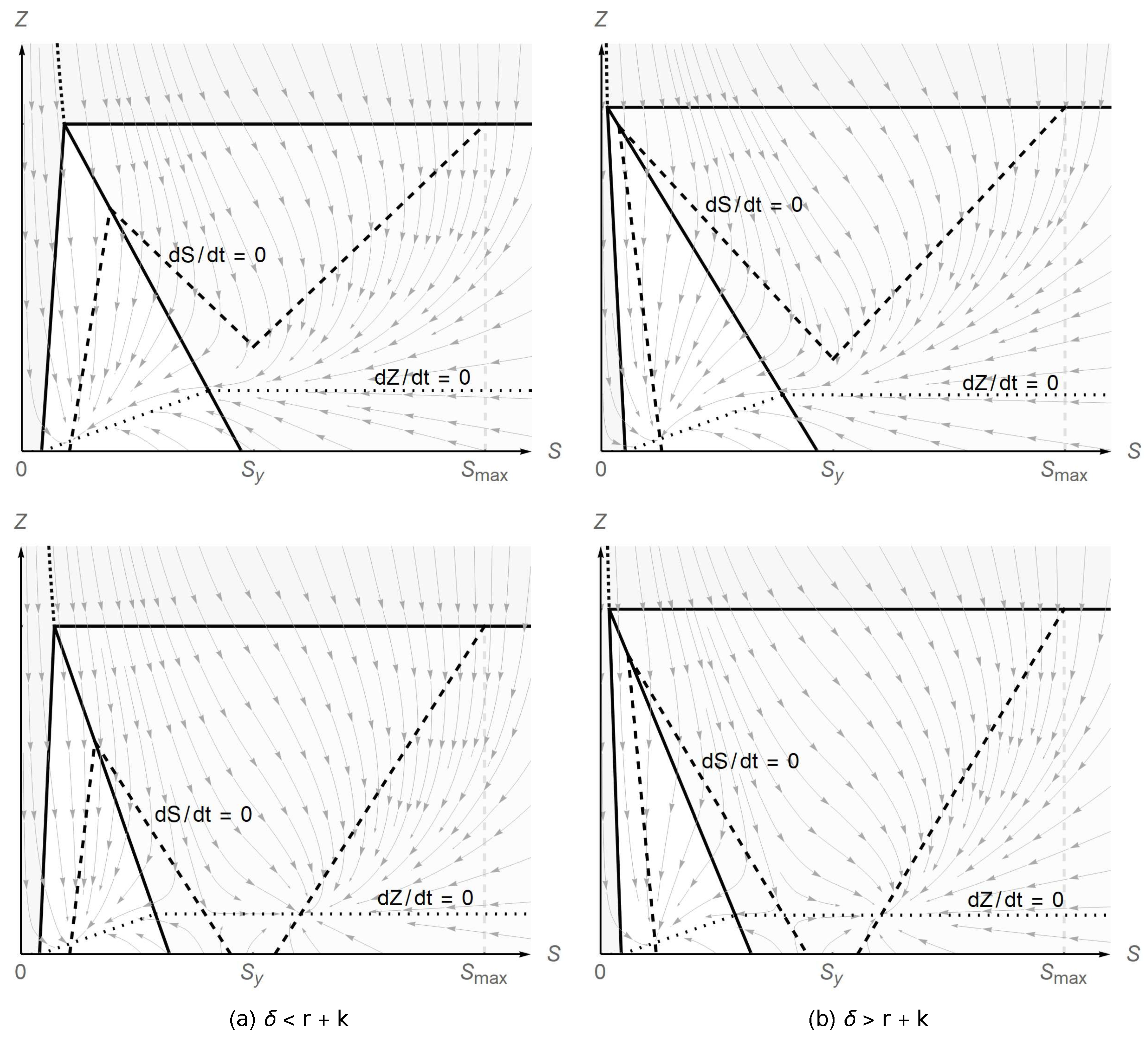
The cases of unique and multiple steady states are illustrated in the diagrams in Figure 4, which also show the equilibrium trajectories in the $(S,Z)$ plane. These trajectories are obtained by using the differential equation system resulting from replacing $q^{*}(S,Z)$ in (11) into (2) and (3). For a given initial state, the equilibrium strategy may shift from one to another as the values of the state variables cross the thresholds between the regions.

Figure 4. Sample equilibria with unique and multiple steady states.

The continuity of $V(S,Z)$ on the boundary cases ensures a smooth transition between the regions with continuous $q^{*}(S,Z)$; consequently, the strategies $q_i(t)=q^{*}(S(t),Z(t)),\forall i$ converge to a steady state with $\underset{t\to +\infty }{lim}{q}^{*}(t)>0$ for all initial states and constitute a symmetric feedback–Nash equilibrium.

We now investigate how the equilibrium responses to marginal increases in asset and pollution stocks vary with the changes in the parameter values. In the following proposition, we analyze these comparative statics for the number of players (n), the marginal damage coefficient ($\varphi$), and the intrinsic growth rate of the asset $(\delta )$.

Proposition 1.

The partial derivatives of coefficients of the equilibrium strategy given in (11) with respect to the selected parameters have the following signs:

$$\begin{array}{cc}\hfill & sign\left(\frac{\partial c_S}{\partial n}\right)<0;sign\left(\frac{\partial c_Z}{\partial n}\right)=sign(k+r-\delta );sign\left(\frac{\partial {\overline{c}}_Z}{\partial n}\right)>0;\hfill \\ \hfill & sign\left(\frac{\partial c_S}{\partial \varphi }\right)>0;sign\left(\frac{\partial c_Z}{\partial \varphi }\right)=sign(\delta -k-r);sign\left(\frac{\partial {\overline{c}}_Z}{\partial \varphi }\right)<0;\hfill \\ \hfill & sign\left(\frac{\partial c_S}{\partial \delta }\right)>0;sign\left(\frac{\partial c_Z}{\partial \delta }\right)>0;sign\left(\frac{\partial {\overline{c}}_Z}{\partial \delta }\right)=0.\hfill \end{array}$$

Proof. 

See Appendix C. □

The results of Proposition 1 can be summarized as follows: the equilibrium response to an increase in asset stock is lower if the number of players is higher, and the response to an increase in pollution stock depends on $sign(k+r-\delta )$. Recall that $sign(c_Z)=sign(\delta -k-r)$; then, with a higher number of players, the equilibrium response to higher pollution is to decrease exploitation less for $\delta <k+r$ and increase exploitation less for $\delta >k+r$. The results are reversed for the marginal damage parameter. When the growth rate of the asset is higher, the response to an increase in asset stock is higher and the response to an increase in pollution stock is also higher, which is in contrast with the effects of the other parameters.

Another example in which the qualitative properties differ is the case of a monopoly. The following proposition presents the result in this case:

Proposition 2.

Under Assumptions 1 and 2, for a monopoly ($n=1$), the optimal solution includes only one stable steady state, which is in region $R_A$.

Proof. 

See Appendix D. □

Proposition 2 shows that, in the monopoly case, the steady state ${\xi }_S$ lies on the boundary $Z=Z_S^A(S)$ and coincides with the unstable steady state in $R_A$, i.e., ${\xi }_S={\xi }_{A1}$. Hence, for a monopoly, this point is unstable but it is sustainable. Analysis regarding the stability of the other steady state in $R_A$ (${\xi }_{A2}$) remains valid, and thus, ${\xi }_{A2}$ is the only steady state that is asymptotically stable. Therefore, for a monopoly, the optimal solution includes two steady states with one of them stable and the other one unstable but sustainable.

4. Concluding Remarks

We characterized the symmetric feedback–Nash equilibrium and showed its existence within a certain range of model parameters given in Assumptions 1 and 2. The equilibrium path always reaches a steady state that is sustainable. For a set of parameters outside this range, there may still exist local equilibria for some levels of asset–pollution stock pairs.

The framework we present includes various simplifications and abstractions, which made the characterization of the equilibrium more conveniently tractable. We introduced the pollution externalities in a simple way in order to guarantee that variations in the equilibrium results between the outcomes with and without pollution externalities could be studied through a single exogenous parameter.

The methodology used to characterize the equilibrium can be applied in problems involving similar features by considering different objective functions and state dynamics. Some examples are the issues relating to the open-access fisheries shared by multiple countries, analysis of cooperation and stability of coalitions, welfare analysis, spillover effects, and the interactions between other possible state variables and the asset stock.

Appendix A.1. Some Preliminaries

A symmetric equilibrium exists if there exists a function $V_i(S,Z)=V(S,Z)\forall i$ that is continuous and continuously differentiable in S and Z, which satisfies the HJB equation in (5), the first-order condition in (7), and the terminal condition ${lim}_{t\to +\infty }{e}^{-rt}V(S(t),Z(t))=0$ for every admissible trajectory (see [40,41]). Due to the nonnegativity restriction on $q_i$ in problem (4), we consider the two following cases:

$$q^{*}(S,Z)>0\mathrm{and}{q}^{*}(S,Z)=0.$$

Moreover, the constraint $q_i(t)\le MS(t)$ in (4) guarantees that the asset stock S cannot be negative.

In order to characterize an equilibrium strategy $q^{*}(S,Z)$ that is defined for the whole state space $(S,Z)\in {\mathbb{R}}_{+}^2$ which converges to a stable steady state with $\underset{t\to +\infty }{lim}(q^{*}(S(t),Z(t))>0)$, we look for the parameter constellations under which the following two conditions are satisfied:

• $q^{*}(0,Z)=0,\forall Z\ge 0$, which is to ensure that asset exhaustion never occurs and there exist steady state(s) with positive asset level.
• $\partial V(S,Z)/\partial S=0,\forall S\ge S_y$, which is to ensure the continuity of $V(S,Z)$ on $S=S_y$ where the asset growth function $f(S_y)$ is not continuously differentiable.

More specifically,

• if $q^{*}(0,Z)=0,\forall Z\ge 0$ is not satisfied, then $\exists Z\ge 0|q^{*}(0,Z)>0$ and then there may exist an initial state $(S(0),Z(0))$ such that $\underset{t\to +\infty }{lim}(S(t),Z(t))=(0,0)$ and $\underset{t\to +\infty }{lim}(q^{*}(S(t),Z(t))=0$; then, $q^{*}(S,Z)$ would not be a feedback–Nash equilibrium that includes stable steady state(s) with positive asset levels.
• if $(\partial V(S,Z)/\partial S=0\forall S\ge S_y)$ is not satisfied, then the discontinuity point $f(S_y)$ given in (2) is included in the case $q^{*}(S,Z)>0$ and $\partial V(S,Z)/\partial S>0$. For this reason, we cannot find a function that is continuously differentiable in S, and $q^{*}(S,Z)$ does not satisfy the HJB equation for $S\ge S_y$; thus, in that case, $V(S,Z)$ together with $q^{*}(S,Z)$ do not fulfill any currently known sufficient condition.

In the following subsections, we use the methods developed in the literature to study the cases given in Definition 1. We focus on linear strategies, obtain the function $V(S,Z)$, and analyze a number of closed-form formulas to identify the restrictions on the model parameters under which the conditions discussed above are satisfied, which allows us to characterize the equilibrium.

Appendix A.2. Case with Positive Exploitation ($Q^{*}(S,Z)>0$)

Since the model is linear-quadratic, we make the informed guess that, within an interior solution ($q^{*}(S,Z)>0$), the value function is a polynomial of degree 2 in S and Z. We consider the function $W(S,Z)$ given in Equation (23).

The maximized HJB equation is obtained by replacing $q^{*}(S,Z)$ in (7) into (5). Using $W(S,Z)$ results in an equation that is a polynomial of degree 2 in S and Z. We then apply the method of undetermined coefficients (see [41]) by identification, and after simplifications, the system of equations in $(A,B,C,D,E,F)$ is written as follows:

$$\begin{array}{cccc}\hfill & A=\frac{(a+\alpha E-C)\left(a+n^2(\alpha E-C)\right)}{b{(n+1)}^{2}r},\hfill & \hfill B& =\frac{2n^2{(\alpha F-B)}^2}{b{(n+1)}^2(r-2\delta )},\hfill \end{array}$$

(A1)

$$\begin{array}{cccc}\hfill & C=\frac{(\alpha F-B)\left(a(n^2+1)+2n^2(\alpha E-C)\right)}{b{(n+1)}^2(r-\delta )},\hfill & \hfill D& =\frac{2n^2{(\alpha D-F)}^2-b{(n+1)}^2\varphi }{b{(n+1)}^2(2k+r)},\hfill \end{array}$$

(A2)

$$\begin{array}{cccc}\hfill & E=\frac{(\alpha D-F)\left(a(n^2+1)+2n^2(\alpha E-C)\right)}{b{(n+1)}^2(k+r)},\hfill & \hfill F& =\frac{2n^2(\alpha D-F)(\alpha F-B)}{b{(n+1)}^2(k+r-\delta )}.\hfill \end{array}$$

(A3)

Introduce the following changes of variables:

$$c_0=\alpha E-C,c_S=\alpha F-B,c_Z=\alpha D-F.$$

(A4)

Replacing (A4) into the equations for C and E, the term $c_0$ is written as a function of $c_S$ and $c_Z$, and is given in (14). Furthermore, using the equations for $B,D$, and F in (A1)–(A3) with (A4) enables us to write the system of equations for $c_S$ and $c_Z$ as follows:

$$\begin{array}{cc}\hfill & c_S=\alpha \frac{2n^2{c}_Z{c}_S}{b{(n+1)}^2(k+r-\delta )}-\frac{2n^2{c}_S^2}{b{(n+1)}^2(r-2\delta )},\hfill \end{array}$$

(A5)

$$\begin{array}{cc}\hfill & c_Z=\alpha \frac{2n^2{c}_Z^2-b{(n+1)}^2\varphi }{b{(n+1)}^2(2k+r)}-\frac{2n^2{c}_Z{c}_S}{b{(n+1)}^2(k+r-\delta )}.\hfill \end{array}$$

(A6)

Hence, we reduced the six-dimensional equation system in (A1)–(A3) into a system of two equations in $c_S$ and $c_Z$, which contain polynomials of degree 2. Equation (A5) has two solutions for $c_S$, i.e., $\left\{c_S=\frac{1}{2}(2\delta -r)\left(\frac{b{(n+1)}^2}{n^2}+\frac{2\alpha c_Z}{\delta -k-r}\right),c_S=0\right\}$. Inserting these values into (A6) yields four solutions to the system in (A5) and (A6):

• Solution A is written in Equations (12) and (13).
• Solution B is written in Equations (15) and (16).
• Solution $A^{\prime }$ and Solution $B^{\prime }$, which are denoted by ($c_S^{\prime },c_Z^{\prime }$) and (${\overline{c}}_S^{\prime },{\overline{c}}_Z^{\prime }$), are written exactly as in (12), (13), (15), and (16) by inverting the sign of $\lambda$, i.e.,

  $${\lambda }_{A^{\prime }}={\lambda }_{B^{\prime }}=-\sqrt{{\left(b(n+1)(2k+r)\right)}^2+8n^2{\alpha }^{2}b\varphi }.$$

The solutions given above consist only of the exogenously given model parameters. Therefore, all solutions for $W(S,Z)$ can be obtained by replacing (A4) in (A1)–(A3) and by inserting the solutions given in (12)–(16).

In solutions A and $A^{\prime }$, $\partial W(S,Z)/\partial S\ne 0\forall \delta \ne r/2$; thus, they are candidates for the case $q^{*}>0$ and $\partial V(S,Z)/\partial S>0$. In solutions B and $B^{\prime }$, we have $\partial W(S,Z)/\partial S=0$, and they are candidates for the case $q^{*}>0$ and $\partial V(S,Z)/\partial S=0$. Therefore, we consider solutions A and $A^{\prime }$ for the function $W(S,Z)$ given in (23), and for solutions B and $B^{\prime }$, where ${\overline{c}}_S={\overline{c}}_S^{\prime }=0$, we define the function denoted by $\overline{V}(Z)$, which is a polynomial of degree 2 in Z, written in (27). It can be verified that both functions $W(S,Z)$ and $\overline{V}(Z)$ satisfy the HJB equation in (5) for all choices of solutions.

Remark A1.

In the limit case where $\varphi \to 0$, the problem reduces to a game with one state variable (S). Solution A reduces to $c_Z=0$, $c_S=(2\delta -r)\frac{b{(1+n)}^2}{2n^2}$, and $c_0=\frac{a\left(1+n^2\right)}{2n^2\delta }(r-2\delta )$, which results in $D=E=F=0$, and $B=-c_S=(r-2\delta )\frac{b{(1+n)}^2}{2n^2}$, $C=-c_0=\frac{a\left(1+n^2\right)}{2n^2\delta }(2\delta -r)$, $A=\frac{a^2\left(r\left(1+n^2\right)-2\delta \right)\left(r\left(1+n^2\right)-2n^2\delta \right)}{4br{n}^2{(1+n)}^2{\delta }^2}$. Solution B vanishes with ${\overline{c}}_S={\overline{c}}_Z={\overline{c}}_0=0$, which leads to the equilibrium outcome of the static Cournot oligopoly, i.e., $\overline{V}(Z)=\frac{a^2}{b{(1+n)}^{2}r}$ and $q^{*}=\frac{a}{b(1+n)}$. These outcomes are identical to their corresponding terms in the solution provided in [11].

The equilibrium strategy is written by using (7) and (A4) with $V(S,Z)=W(S,Z)$:

$$q^{*}(S,Z)=(a+c_0+c_{S}S+c_{Z}Z)/b(n+1),$$

(A7)

which is linear in S and Z. Note that, by using (A4), the RHS of (6) can be written as $MC(S,Z)=-(c_0+c_{S}S+c_{Z}Z)$; hence, these terms correspond to the coefficients of the marginal cost function.

In the following sections, we use the functions $W(S,Z)$ and $\overline{V}(Z)$ to study the two cases where $\partial V/\partial S>0$ and $\partial V/\partial S\ge 0$.

Appendix A.2.1. Case with $Q^{*}(S,Z)>0$ and $\partial V(S,Z)/\partial S>0$

We first obtain the analytical formulation of $R_S$. For $q^{*}(S,Z)>0$, from (A7), we obtain $a>-c_0-c_{S}S-c_{Z}Z$, and for $\partial W(S,Z)/\partial S>0$, we use (A1) to (A4). Since $c_S>0$ in all cases for $\delta >r/2$, writing both inequalities in S enables us to obtain the following region and its boundary cases:

(i) 

$q^{*}(S,Z)>0$ and $\partial V(S,Z)/\partial S>0$ for all $(S,Z)\in R_S$ where $R_S$ is given in (19); the boundary line associated with the first inequality, which is denoted by $Z=Z_0^S(S)$, is written in (37); and the sign of its slope is given by $sign(\frac{d{Z}_0^S(S)}{dS})=sign(-\frac{c_S}{c_Z})$.

• if $r/2<\delta <r+k$, then $\frac{d{Z}_0^S(S)}{dS}>0$;
• if $\delta =r+k$, Equation (37) reduces to $S=-\frac{a+c_0}{c_S}$; and
• if $\delta >r+k$, then $\frac{d{Z}_0^S(S)}{dS}<0$.

(ii) 

The set of points such that $q^{*}(S,Z)=0$ is defined as follows:

$$q^{*}(S,Z)=0\mathrm{if}\left\{(S,Z)|S\le -\frac{a+c_0}{c_S}-\frac{c_Z}{c_S}Z\right\},$$

(A8)

which is obtained by using $a\le \frac{\partial W(S,Z)}{\partial S}-\alpha \frac{\partial W(S,Z)}{\partial Z}$.

(iii) 

The set of points such that $\partial W(S,Z)/\partial S=0$ is given by the linear function in S written in Equation (38), and the sign of its slope is given by $sign(\frac{d{Z}_S^A(S)}{dS})$ = $sign(-\frac{(\delta -r-k)}{(2\delta -r)}\frac{c_S}{c_Z})$. Since $sign(c_Z)$ = $sign(\delta -r-k)$ and $c_S>0$, we have $\frac{d{Z}_S^A(S)}{dS}<0$ in all cases where $\delta >r/2$.

We now calculate the points at which the linear functions obtained for the boundary cases intersect with the $Z=0$ axis and each other, i.e., $Z_0^S(S)=0$, $Z_S^A(S)=0$, and $Z=Z_0^S(S)=Z_S^A(S)$. These formulas are first written in terms of $(c_0,c_S,c_Z)$, and then, after inserting the solutions in (12)–(16), they are written in closed form, using $\lambda$ in (18) to study their signs.

(i) 

$(S_1,0)$: $Z_0^S(S_1)=0$ and $q^{*}(S,0)=0\forall S\le S_1$ where

$$\begin{array}{cc}\hfill S_1=& -\frac{a+c_0}{c_S},\hfill \\ \hfill =& \frac{2a(k+\delta )\left(2br\delta +\left(1+n^2\right)b\left(\delta (2k+r)-2r(k+r)\right)-(n-1)\delta \lambda \right)}{\delta (2\delta -r)(\lambda +b(1+n)(2\delta -r))(\lambda +b(1+n)r)}.\hfill \end{array}$$

(A9)

(ii) 

$(S_2,0)$: $Z_S^A(S_2)=0$ where

$$\begin{array}{cc}\hfill S_2& =-\frac{(2\delta -r)\left(a\left(1+n^2\right)+2n^2{c}_0\right)}{2n^2(\delta -r)c_S},\hfill \\ \hfill & =\frac{4ab\left(1+n^2\right)(k+r)(k+\delta )}{\delta (\lambda +b(1+n)r)(\lambda +b(1+n)(2\delta -r))}>0\mathrm{if}\delta >r/2.\hfill \end{array}$$

(A10)

(iii) 

$(S_3,Z_3)$: $Z_0^S(S_3)=Z_S^A(S_3)=Z_3$ is written in Equations (35) and (36) and note that $Z_3>0$.

By using (A9) and (A10), the difference $S_2-S_1$ is given by

$$S_2-S_1=\frac{2a\left(b\left(2k\left(1+n^2\right)+r\left(1+3n^2\right)\right)+(n-1)\lambda \right)(k+\delta )}{(2\delta -r)(\lambda +b(1+n)r)(\lambda +b(1+n)(2\delta -r))}>0\mathrm{if}\delta >r/2.$$

(A11)

Thus, for $\delta >r/2$, $Z=Z_S^A(S)$ intersects with the $Z=0$ axis at $S_2>0$ and $S_2>S_1$. By using (A9), we obtain the conditions under which $S_1>0$:

$$\begin{array}{cc}\hfill & \delta >\frac{r\left(1+n^2\right)}{2},\hfill \end{array}$$

(A12)

$$\begin{array}{cc}\hfill & \varphi <{\varphi }_1.\hfill \end{array}$$

(A13)

where ${\varphi }_1$ is given in (8).

For $\delta \le r+k$, $S_3>0$ if (A12) and (A13) are satisfied, and for $\delta >r+k$, $S_3>0$ if

$$\begin{array}{cc}\hfill & \delta <\frac{k\left(n^2+1\right)}{n^2-1},\hfill \end{array}$$

(A14)

$$\begin{array}{cc}\hfill & \varphi <{\varphi }_2,\hfill \end{array}$$

(A15)

where ${\varphi }_2$ is given in (9), and note that this condition is more strict than the one in (8) (i.e., ${\varphi }_2<{\varphi }_1$).

Lemma A1.

Suppose that Assumptions 1 and 2 are satisfied. For all $(S,Z)\in R_S$, the function $V(S,Z)=W(S,Z)$ satisfies the HJB Equation (5) and the strategies $q_i=q^{*}(S,Z),\forall i$ given in (11) satisfy (7) with $q^{*}(S,Z)>0$ and $\partial V(S,Z)/\partial S>0$.

Proof. 

The sign analysis conducted in (A9) to (A15) shows that, if the conditions given in Assumptions 1 and 2 are satisfied, then we have $0<S_1<S_2<S_y$ and $S_3>0,Z_3>0$. We study the slopes of the two boundary lines of $R_S$ for each case. The slope of $Z=Z_0^S(S)$ depends on $sign(-\frac{c_S}{c_Z})$, and the slope $d{Z}_S^A(S)/dS<0$ if $\delta >r/2$; then, the three cases are written as follows:

Case 1: 

$\delta <r+k$: In this case $d{Z}_0^S(S)/dS>0$ and $d{Z}_S^A(S)/dS<0$. If $S_1>0$ ((A12) and (A13)), then $q^{*}(S,Z)=0\forall (S,Z)|S\le S_1$. In addition, if $S_2<S_y$, then $(S,Z)\notin R_S\forall (S,Z)|S\ge S_2$ (see Figure 1 and Figure 2a). The function $W(S,Z)$ satisfies the HJB Equation (5) and condition (7) with $q^{*}(S,Z)>0\forall (S,Z)\in R_S$.

Case 2: 

$\delta =r+k$: In this case $c_Z=0$ and the boundary case $q^{*}(S,Z)=0$ reduces to $(S_1,Z)\forall Z\le Z_3$. We have the same result as the previous case. If $S_1>0$ and $S_2<S_y$, then the function $W(S,Z)$ satisfies the HJB Equation (5) and condition (7) with $q^{*}(S,Z)>0\forall (S,Z)\in R_S$.

Case 3: 

$\delta >r+k$: In this case $d{Z}_0^S(S)/dS<0$ and $d{Z}_S^A(S)/dS<0$, and hence, both boundary lines decrease in S. The difference in their slopes is given by $d{Z}_0^S(S)/dS-d{Z}_S^A(S)/dS=-\frac{c_S}{c_Z}\frac{(\delta +k)}{(2\delta -r)}$. Since for $\delta >r+k$ we have $c_S>0$ and $c_Z>0$, the slopes compare as follows:

$$\frac{d{Z}_0^S(S)}{dS}<\frac{d{Z}_S^A(S)}{dS}<0\mathrm{if}\delta >r/2,$$

(A16)

thus, $Z_0^S(S)$ is steeper than $Z_S^A(S)$, and $Z_3>0$, which can also be seen in (36). If $S_3>0$ ((A14) and (A15)) and $S_2<S_y$ are satisfied, then $q^{*}(S,Z)=0\forall S\le S_3\mathrm{and}\forall Z\ge 0$ (see Figure 2b), and the function $W(S,Z)$ satisfies the HJB Equation (5) and condition (7) with $q^{*}(S,Z)>0\forall (S,Z)\in R_S$.

 □

Note that, when using (19), we eliminate the possibility of choosing solution A for $\delta <r/2$ (where $c_S<0$) and solution $A^{\prime }$ for $r/2<\delta <r+k$ (where $c_S^{\prime }<0$ and $c_Z^{\prime }>0$). In these cases, the inequalities in (19) and (A8) change their directions. In step (A16), we eliminate the possibility of choosing solution $A^{\prime }$ for $\delta <r/2$ (where $c_S^{\prime }>0$ and $c_Z^{\prime }>0$), as it leads to $\frac{d{Z}_S^A(S)}{dS}<\frac{d{Z}_0^S(S)}{dS}<0$, which does not allow to characterize a feedback–Nash equilibrium.

Appendix A.2.2. Case with $Q^{*}(S,Z)>0$ and $\partial V(S,Z)/\partial S>0$

We now consider the function $V(S,Z)=\overline{V}(Z)$ given in (27), and by using $a>-\alpha \frac{\partial \overline{V}(Z)}{\partial Z}$, which is given by $a>-\alpha (\overline{D}Z+\overline{E})$ with (19), (28), and (38), we have

(i) 

$q^{*}(S,Z)>0$ and $\partial V(S,Z)/\partial S=0$ for all $(S,Z)\in R_A$, where $R_A$ is given in (20).

(ii) 

The set of points such that $q^{*}(S,Z)=0$ and $\partial V(S,Z)/\partial S=0$ is written in Equation (39), which is obtained by using $a=-\alpha \frac{\partial \overline{V}(Z)}{\partial Z}$ and (28). The explicit form of $Z_0^A$ equals the constant $Z_3$ given in (36).

Lemma A2.

Suppose that Assumptions 1 and 2 are satisfied. For $(S,Z)\in R_S\cup R_A$ where $V(S,Z)=\left\{W(S,Z)\mathrm{if}(S,Z)\in R_S,\overline{V}(Z)\mathrm{if}(S,Z)\in R_A\right\}$, the strategies $q_i=q^{*}\forall i$ given in (11) satisfy the HJB Equation (5) and condition (7) with $q^{*}(S,Z)>0$ and the function $V(S,Z)$ is continuously differentiable $\forall (S,Z)\in R_S\cup R_A$.

Proof. 

The functions $W(S,Z)$ and $\overline{V}(Z)$ are polynomials of degree 2 and thus continuously differentiable in S and Z $\forall (S,Z)\in R_S$ and $\forall (S,Z)\in R_A$, respectively. For continuity of $V(S,Z)$ on the boundary, as $(S,Z)\to (\widehat{s},\widehat{z})|\widehat{z}=Z_S^A(\widehat{s})$:

$$\begin{array}{cc}\hfill \underset{(S,Z)\to (\widehat{s},\widehat{z})}{lim}W(S,Z)& =\left(A-\frac{C^2}{2B}\right)+\left(\frac{D}{2}-\frac{F^2}{2B}\right){\widehat{z}}^2+\left(E-\frac{CF}{B}\right)\widehat{z},\hfill \end{array}$$

(A17)

$$\begin{array}{cc}\hfill \underset{(S,Z)\to (\widehat{s},\widehat{z})}{lim}\overline{V}(Z)& =\overline{A}+\frac{\overline{D}}{2}{\widehat{z}}^2+\overline{E}\widehat{z}.\hfill \end{array}$$

(A18)

where (A17) is obtained by using $S=-C/B-ZF/B$ (where $\partial W(S,Z)/\partial S=0$). By using (24) to (28), it can be verified that

$$\overline{A}=A-\frac{C^2}{2B};\frac{\overline{D}}{2}=\left(\frac{D}{2}-\frac{F^2}{2B}\right);\overline{E}=\left(E-\frac{CF}{B}\right),$$

(A19)

Therefore, ${lim}_{(S,Z)\to (\widehat{s},\widehat{z})}W(S,Z)={lim}_{(S,Z)\to (\widehat{s},\widehat{z})}\overline{V}(Z)$ for $\widehat{z}=Z_S^A(\widehat{s})$, and thus, $V(S,Z)$ is continuous on $\left\{(S,Z)|Z=Z_S^A(S)\right\}$.

Note that the four solutions to the system in (A5) and (A6) are paired such that (A19) is true for solutions (A and B) and ($A^{\prime }$ and $B^{\prime }$) while (A19) is not true for ($A^{\prime }$ and B) and (A and $B^{\prime }$); therefore, in order to have a function that is continuously differentiable on the boundary where ${lim}_{(S,Z)\to (\widehat{s},\widehat{z})}\partial W(S,Z)/\partial S=0$, either one of the pair of solutions must be selected.

By the definition of $Z=Z_S^A(S)$ given in (38), ${lim}_{(S,Z)\to (\widehat{s},\widehat{z})}\frac{\partial W(S,Z)}{\partial S}=0$, and $\frac{\partial \overline{V}(Z)}{\partial S}=0$; hence $\partial V(S,Z)/\partial S$ is continuous on $\left\{(S,Z)|Z=Z_S^A(S)\right\}$. Further, ${lim}_{(S,Z)\to (\widehat{s},\widehat{z})}\frac{\partial W(S,Z)}{\partial Z}={lim}_{(S,Z)\to (\widehat{s},\widehat{z})}\frac{\partial \overline{V}(Z)}{\partial Z}$ since $(D-F^2/B)=\overline{D}$ by (A19), and thus, $\partial V(S,Z)/\partial Z$ is continuous on $Z=Z_S^A(S)$ and $q^{*}(S,Z)$ is continuous on $Z=Z_S^A(S)$, which can also be shown by using the solutions given in (12)–(16).

By using Lemma A1, $d{Z}_S^A(S)/dS<0$ in all cases with $S_2>0$. If $S_2<S_y$, then $(S_y,Z)\in R_A$$\forall Z\in \left[0,Z_0^A\right)$. For $(S,Z)\in R_A$, we have $V(S,Z)=\overline{V}(Z),$ which does not depend on S; hence, the point $S=S_y$ where $f^{\prime }(S)$ is not continuous does not affect the continuity of $V(S,Z)$. Therefore, the function $V(S,Z)$ is continuously differentiable in S and Z and satisfies the HJB Equation (5) and condition (7) with $q^{*}(S,Z)>0$ $\forall (S,Z)\in R_S\cup R_A$. □

To constitute a Nash equilibrium, the strategies are required to be defined for the whole state space; hence, we study the case $q^{*}(S,Z)=0$ in the next subsection.

Appendix A.3. Case with No Exploitation ($Q^{*}(S,Z)=0$)

By combining the results in (39) and (A8), we obtain the set of points such that $q^{*}(S,Z)=0$ ($R_0$) given in (21). The value function for this region, denoted by $V_0(S,Z)$, must satisfy the HJB equation in (5) with $q_i=0$ for $i\in \left\{1,..,n\right\}$, i.e.,

$$r{V}_0(S,Z)=-\frac{\varphi }{2}{Z}^2+\delta S\frac{\partial V_0(S,Z)}{\partial S}-kZ\frac{\partial V_0(S,Z)}{\partial Z}.$$

(A20)

The above equation is a first-order linear partial differential equation (PDE), and $V_0(S,Z)$ must be continuously differentiable in $R_0$ and on its boundary cases. In order to obtain this function, we begin by deriving the boundary case associated to a given point in $R_0$.

Under Assumptions 1 and 2, for $(S(0),Z(0))\in R_0$, $\exists \widehat{t}\ge 0$ such that $Z(\widehat{t})=Z_0(S(\widehat{t}))$, where $Z_0(S)$ denotes either the boundary between $R_S$ and $R_0$ (i.e., $Z_0^S(S)$) or the boundary between $R_A$ and $R_0$ (i.e., $Z_0^A$). This point is denoted by $(\widehat{s},\widehat{z})=(S(\widehat{t}),Z(\widehat{t}))$ and found by solving the following system of equations:

$$\begin{array}{cc}\hfill & \widehat{z}=Z(\widehat{t})=Z{e}^{-k\widehat{t}},\widehat{s}=S(\widehat{t})=S{e}^{\delta \widehat{t}},\hfill \end{array}$$

(A21)

$$\begin{array}{cc}\hfill & \mathrm{such}\mathrm{that}Z(\widehat{t})=Z_0(S(\widehat{t}))\mathrm{and}\widehat{t}\ge 0,\hfill \end{array}$$

(A22)

where (A21) is found by using $q_i=0\forall i$, which implies $\dot{S}(t)=\delta S(t)$ and $\dot{Z}(t)=-kZ(t)$. By using (21), there are three cases in which Equation (A22) holds true:

(i) 

$\widehat{z}=Z_0^S(\widehat{s})$; then, the point $(\widehat{s},\widehat{z})$ is given by the system of equations written in Equation (31).

(ii) 

$\widehat{z}=Z_0^A$ with $S\ge S_3$; then, the point $(\widehat{s},\widehat{z})$ is given by

$$\widehat{S}(S,Z)=S{\left(\frac{Z}{Z_0^A}\right)}^{\frac{\delta }{k}}\ge S_3,\widehat{Z}(S,Z)=Z_0^A.$$

(A23)

(iii) 

$Z(0)=0$; then, the point $(\widehat{s},\widehat{z})$ is given by

$$\widehat{S}(S,0)=-\frac{a+c_0}{c_S},\widehat{Z}(S,0)=0\mathrm{for}S\le -\frac{a+c_0}{c_S}.$$

(A24)

The system in (31) does not have an analytical solution, and the pair of equations are written as implicit functions denoted by $\widehat{S}(S,Z)$ and $\widehat{Z}(S,Z)$. For a fixed point on the boundary $z_0=Z_0^S(s_0)$, ${lim}_{(S,Z)\to (s_0,z_0)}(\widehat{S}(S,Z),\widehat{Z}(S,Z))=(s_0,z_0)$, which will be used later. The functions $\widehat{S}(S,Z)$ and $\widehat{Z}(S,Z)$ have to be computed numerically except some special cases given below:

Remark A2.

There are special cases where (31) has an analytical solution:

$$\begin{array}{cc}\hfill & if\delta =kthen\left\{\begin{array}{c}\widehat{S}(S,Z)=\left(\sqrt{\left(a+c_0\right){}^2-4SZ{c}_Z{c}_S}-\left(a+c_0\right)\right)/(2c_S),\hfill \\ \widehat{Z}(S,Z)=-\left(\sqrt{\left(a+c_0\right){}^2-4SZ{c}_Z{c}_S}+\left(a+c_0\right)\right)/(2c_Z),\hfill \end{array}\right.\hfill \end{array}$$

(A25)

$$\begin{array}{cc}\hfill & if\delta =r+kthen\left\{\begin{array}{c}\widehat{S}(S,Z)=-\frac{a+c_0}{c_S},\hfill \\ \widehat{Z}(S,Z)=Z\left(-\frac{S{c}_S}{a+c_0}\right){}^{k/\delta },\hfill \end{array}\right.\hfill \end{array}$$

(A26)

Since $Z(t)$ decreases (by (A21)), for $(S(0),Z(0))\in R_0$ where $Z(0)<Z_0^A$, we have $\exists \widehat{t}\ge 0$ such that $Z(\widehat{t})=\widehat{Z}(S(0),Z(0))=Z_0^S(\widehat{S}(S(0),Z(0)))$. However, for $Z(0)\ge Z_0^A$, depending on the position of $(S(0),Z(0))$, $Z(\widehat{t})$ may lie on $Z=Z_0^S(S)$ or $Z=Z_0^A$. In order to precisely determine the boundary associated to every point in $R_0$, we first obtain the curve associated with the intersection of the boundary cases of $R_S$ (denoted by $(S,Z)=(S_3,Z_3)$ given in Equations (35) and (36) and recall that $Z_3=Z_0^A$). The set of points $(S(0),Z(0))\in R_0$ such that $\exists \widehat{t}\ge 0$ where $(S(\widehat{t}),Z(\widehat{t}))=(S_3,Z_3)$ is given by the curve denoted by $Z=\mathsf{\Psi }(S)$ that is written in Equation (34), which is found by solving (A21) with $(\widehat{s},\widehat{z})=(S_3,Z_3)$, and note that $d\mathsf{\Psi }(S)/dS=-\frac{k}{\delta }\frac{S_3{Z}_3}{S^2}{\left(\frac{S_3}{S}\right)}^{\frac{k}{\delta }-1}<0$. By using (34), we define the partitions of region $R_0$, denoted by $R_0^W$ and $R_0^{\overline{V}}$, given in Equations (32) and (33).

Consider a point $(S(0),Z(0))=(s_0,z_0)$ such that $z_0=\mathsf{\Psi }(s_0)$, where $s_0<S_3$ and $z_0>Z_3$. It satisfies $(\widehat{S}(s_0,z_0),\widehat{Z}(s_0,z_0))=(S_3,Z_3)$. Denote by $t=t_0$ such that $(S(t_0),Z(t_0))=(S_3,Z_3)$. By using (A21), we obtain $t_0=\frac{1}{k}log\left(\frac{z_0}{Z_3}\right)=\frac{1}{\delta }log\left(\frac{S_3}{s_0}\right)>0$. Then:

• for $(S(0),Z(0))=(s^{\prime },z_0)\in R_0^W$ where $s^{\prime }<s_0$, we have $(S(t_0),Z(t_0))=(S(t_0),Z_3)$ with $S(t_0)<S_3$; hence $(S(t_0),Z_3)\in R_0$, $(S(t_0),Z_3)\notin R_S$, and $(S(t_0),Z_3)\notin R_A$. Then, $\widehat{z}=Z_0^S(\widehat{s})$, and the point $(\widehat{s},\widehat{z})$ is given by (31).
• for $(S(0),Z(0))=(s^{″},z_0)\in R_0^{\overline{V}}$ where $s^{″}>s_0$, we have $(S(t_0),Z(t_0))=(S(t_0),Z_3)$ with $S(t_0)>S_3$; hence the point $(\widehat{s},\widehat{z})$ is given by (A23).

To summarize, if $(S,Z)\in R_0^W$, then $\widehat{Z}(S,Z)=Z_0^S(\widehat{S}(S,Z))$, and if $(S,Z)\in R_0^{\overline{V}}$, then $\widehat{Z}(S,Z)=Z_0^A$.

Since we obtained the boundary case associated with every point in $R_0$, by applying the method of characteristics (see [43]), we obtain the solution to (A20) given in the following lemma:

Lemma A3.

The value function in $R_0$ is written in Equation (29). The function $V_0(S,Z)$ is continuously differentiable in S and Z $\forall (S,Z)\in R_0$ and on the boundary cases of $R_0$.

Proof. 

We first consider Equation (A20) such that $V(S,\widehat{z})=\mathsf{\Theta }(S,\widehat{z})$ with a constant $\widehat{z}$, where $\mathsf{\Theta }(S,Z)$ is an analytical function of S and Z, which is a Cauchy problem. Suppose that a function u, which is parameterized by $\tau$, is a solution to Equation (A20) such that $u(\tau )=u(S(\tau ),Z(\tau ))=V(S(\tau ),Z(\tau ))$. Introduce the system of ordinary differential equations (ODEs), which are called the characteristic system for the PDE in (A20):

$$\begin{array}{cc}\hfill & \frac{du}{d\tau }=ru+\frac{\varphi }{2}{Z}^2;\frac{dS}{d\tau }=\delta S;\frac{dZ}{d\tau }=-kZ\mathrm{such}\mathrm{that},\hfill \end{array}$$

(A27)

$$\begin{array}{cc}\hfill & u(0)=\mathsf{\Theta }(\widehat{s},\widehat{z});S(0)=\widehat{s};Z(0)=\widehat{z}.\hfill \end{array}$$

(A28)

Solving the last two equations in (A27) with their initial conditions results in

$$\begin{array}{c}\hfill S(\tau )=\widehat{s}{e}^{\delta \tau },Z(\tau )=\widehat{z}{e}^{-k\tau }.\end{array}$$

(A29)

By solving for $e^{\tau }$ and $\widehat{s}$, we obtain $\tau (S,Z)$ and $\widehat{S}(S,Z)$ that satisfy (A29):

$$\begin{array}{c}\hfill e^{\tau }={\left(\frac{Z(\tau )}{\widehat{z}}\right)}^{-\frac{1}{k}};\widehat{s}=S(\tau )e^{-\delta \tau }=S(\tau ){\left(\frac{Z(\tau )}{\widehat{z}}\right)}^{\frac{\delta }{k}}.\end{array}$$

(A30)

We insert $Z(\tau )$ given in (A29) into the first ODE in (A27) and obtain the following equation:

$$\begin{array}{c}\hfill \frac{du}{d\tau }=ru+\frac{\varphi }{2}{\widehat{z}}^2{e}^{-2k\tau }.\end{array}$$

(A31)

Solving (A31) with its initial condition in (A28) yields

$$u(\tau )=e^{r\tau }\mathsf{\Theta }(\widehat{s},\widehat{z})+e^{r\tau }\frac{\varphi {\widehat{z}}^2}{2(2k+r)}\left(1-e^{-(2k+r)\tau }\right).$$

(A32)

Replacing (A30) into (A32) yields

$$u(S(\tau ),Z(\tau ))={\left(\frac{Z(\tau )}{\widehat{z}}\right)}^{-\frac{r}{k}}\mathsf{\Theta }\left(S(\tau ){\left(\frac{Z(\tau )}{\widehat{z}}\right)}^{\frac{\delta }{k}},\widehat{z}\right)+\frac{\varphi Z{(\tau )}^2}{2(2k+r)}\left({\left(\frac{Z(\tau )}{\widehat{z}}\right)}^{-\frac{2k+r}{k}}-1\right);$$

(A33)

Hence, we obtained the solution to (A20), which is verified for any analytical function $\mathsf{\Theta }(S,Z)$. Further, in order to satisfy the boundary conditions in (A21) and (A22) $\forall (S,Z)\in R_0$, we replace $\widehat{z}=\widehat{Z}(S,Z)$ and obtain (29). We then write (A20) by using (29), which simplifies to the following equation:

$$\begin{array}{c}\left(\frac{2}{k\widehat{Z}(.)}{\left(\frac{Z}{\widehat{Z}(.)}\right)}^{-\frac{r}{k}}\right)\left(kZ\frac{\partial \widehat{Z}(.)}{\partial Z}-\delta S\frac{\partial \widehat{Z}(.)}{\partial S}\right)\hfill \\ \hfill \left(r\mathsf{\Theta }(\widehat{S}(.),\widehat{Z}(.))-\left(\delta \widehat{S}(.)\frac{\partial \mathsf{\Theta }(\widehat{S}(.),\widehat{Z}(.))}{\partial S}-k\widehat{Z}(.)\frac{\partial \mathsf{\Theta }(\widehat{S}(.),\widehat{Z}(.))}{\partial Z}-\frac{\varphi }{2}\widehat{Z}{(.)}^2\right)\right)=0.\end{array}$$

(A34)

We showed that, for $(S,Z)\in R_0^W$ where $\mathsf{\Theta }(S,Z)=W(S,Z)$, we have $\widehat{Z}(S,Z)=Z_0^S(\widehat{S}(S,Z))$. For $\widehat{z}=Z_0^S(\widehat{s})$, $W(\widehat{s},\widehat{z})$ satisfies the HJB Equation (5) with $q^{*}(\widehat{s},\widehat{z})=0$, i.e.,

$$rW(\widehat{s},\widehat{z})=\delta \widehat{s}\frac{\partial W(\widehat{s},\widehat{z})}{\partial S}-k\widehat{z}\frac{\partial W(\widehat{s},\widehat{z})}{\partial Z}-\frac{\varphi }{2}{\widehat{z}}^2,$$

(A35)

and for $(S,Z)\in R_0^{\overline{V}}$ where $\mathsf{\Theta }(S,Z)=\overline{V}(Z)$, we have $\widehat{Z}(S,Z)=Z_0^A$. When $\widehat{z}=Z_0^A$, $\overline{V}(\widehat{z})$ satisfies (5) with $q^{*}(\widehat{s},\widehat{z})=0$,

$$r\overline{V}(\widehat{z})=-k\widehat{z}\frac{\partial \overline{V}(\widehat{z})}{\partial Z}-\frac{\varphi }{2}{\widehat{z}}^2.$$

(A36)

For both cases, the third term in (A34) is zero and the equation holds true; hence, the function $V_0(S,Z)$ given in (29) satisfies the HJB equation in (5) with $q_i^{*}=0\forall i$ and $\forall (S,Z)\in R_0$.

For the partial derivatives of $V_0(S,Z)$ with respect to S and Z, by collecting the terms multiplied with $\partial \widehat{Z}(S,Z)/\partial S$ and $\partial \widehat{Z}(S,Z)/\partial Z$, using (A35) and (A36) allows us to simplify to the following:

$$\frac{\partial V_0(S,Z)}{\partial S}={\left(\frac{Z}{\widehat{Z}(.)}\right)}^{\frac{\delta -r}{k}}\frac{\partial \mathsf{\Theta }(\widehat{S}(.),\widehat{Z}(.))}{\partial S},$$

(A37)

$$\frac{\partial V_0(S,Z)}{\partial Z}={\left(\frac{Z}{\widehat{Z}(.)}\right)}^{-\frac{k+r}{k}}\frac{\partial \mathsf{\Theta }(\widehat{S}(.),\widehat{Z}(.))}{\partial Z}-\frac{\varphi Z}{2k+r}\left(1-{\left(\frac{Z}{\widehat{Z}(.)}\right)}^{-\frac{2k+r}{k}}\right).$$

(A38)

The function $V_0(S,Z)$ is continuously differentiable in S and Z$\forall (S,Z)\in R_0^W$, $\forall (S,Z)\in R_0^{\overline{V}}$, and $\forall (S,Z)|Z=\mathsf{\Psi }(S)$, since on this curve, $\widehat{Z}(S,Z)=Z_3$ and $W(S_3,Z_3)=\overline{V}(Z_3)$.

• Continuity of $V(S,Z)$ on the boundary cases of $R_0$:

There are two cases: $(a)$$(S,Z)=(S,Z_0^S(S))$ and $(b)$$(S,Z)=(S,Z_0^A)$ with $S\ge S_3$.

(a) 

$(S,Z)=(S,Z_0^S(S))$

On this boundary case, $\widehat{z}=Z_0^S(\widehat{s})$ and we have ${lim}_{(S,Z)\to (\widehat{s},\widehat{z})}(\widehat{S}(S,Z),\widehat{Z}(S,Z))=(\widehat{s},\widehat{z})$,

$$\underset{(S,Z)\to (\widehat{s},\widehat{z})}{lim}{V}_0(S,Z)=W(\widehat{s},\widehat{z}),$$

(A39)

Thus, $V(S,Z)$ is continuous on $Z=Z_0^S(S)$. For continuity of its partial derivatives, by using (A37) and (A38), we obtain

$$\underset{(S,Z)\to (\widehat{s},\widehat{z})}{lim}\frac{\partial V_0(S,Z)}{\partial S}=\frac{\partial W(\widehat{s},\widehat{z})}{\partial S},\underset{(S,Z)\to (\widehat{s},\widehat{z})}{lim}\frac{\partial V_0(S,Z)}{\partial Z}=\frac{\partial W(\widehat{s},\widehat{z})}{\partial Z};$$

(A40)

Hence, $V(S,Z)$ is continuously differentiable in S and Z on $Z=Z_0^S(S)$.

(b) 

$(S,Z)\in (S,Z_0^A)$ with $S\ge S_3$:

On this boundary case, we have ${lim}_{(S,Z)\to (\widehat{s},\widehat{z})}(\widehat{S}(S,Z),\widehat{Z}(S,Z))=(\widehat{s},Z_0^A)$ with $\widehat{s}\ge S_3$. For continuity, we have

$$\underset{(S,Z)\to (\widehat{s},\widehat{z})}{lim}{V}_0(S,Z)=\overline{V}(\widehat{z}),$$

(A41)

Thus, $V(S,Z)$ is continuous on $Z=Z_0^A$. For continuity of its partial derivatives, by using (A38), we have

$$\underset{(S,Z)\to (\widehat{s},\widehat{z})}{lim}\frac{\partial V_0(S,Z)}{\partial S}=\frac{\partial \overline{V}(\widehat{z})}{\partial S}=0,\underset{(S,Z)\to (\widehat{s},\widehat{z})}{lim}\frac{\partial V_0(S,Z)}{\partial Z}=\frac{\partial \overline{V}(\widehat{z})}{\partial Z},$$

(A42)

Thus, $V(S,Z)$ is continuously differentiable on $Z_0^A$ with $S\ge S_3$.

Therefore, the function $V_0(S,Z)$ is continuously differentiable in S and Z in $R_0$ and both its boundary cases.

 □

Consequently, by using Lemmas A1–A3, under Assumptions 1 and 2, the function $V(S,Z)$ given in (22) is continuously differentiable in S and Z and satisfies the HJB equation in (5), and the strategy profile $q_i=q^{*}(S,Z)\forall i$ given in (11) satisfies condition (7) for all $(S,Z)\in {\mathbb{R}}_{+}^2$. The terminal condition is satisfied because $\dot{Z}(t)\le -kZ(t)+\alpha Mn{S}_{max}$ and the set of all S is bounded, while the set of all $Z\ge 0$ can be divided into two parts: a bounded interval and a set in which every admissible trajectory Z decreases so every admissible trajectory is bounded. Thus, by continuity of $V(S,Z)$, for any given initial condition $(S(0),Z(0))$, the limit of $V(S(t),Z(t))e^{-rt}$ exists and equals 0. Therefore, $q_i=q^{*}\forall i$ constitutes a symmetric feedback–Nash equilibrium, which proves Theorem 1.

References

- Eriksen, M.; Lebreton, L.C.; Carson, H.S.; Thiel, M.; Moore, C.J.; Borerro, J.C.; Reisser, J. Plastic pollution in the world’s oceans: More than 5 trillion plastic pieces weighing over 250,000 tons afloat at sea. PLoS ONE 2014, 9, e111913. [Google Scholar] [CrossRef] [PubMed]
- Newman, S.; Watkins, E.; Farmer, A.; Ten Brink, P.; Schweitzer, J.P. The economics of marine litter. In Marine Anthropogenic Litter; Bergmann, M., Gutow, L., Klages, M., Eds.; Springer: Cham, Switzerland, 2015; pp. 367–394. [Google Scholar]
- Richardson, K.; Hardesty, B.D.; Wilcox, C. Estimates of fishing gear loss rates at a global scale: A literature review and meta-analysis. Fish Fish. 2019, 20, 1218–1231. [Google Scholar] [CrossRef]
- Gilman, E. Status of international monitoring and management of abandoned, lost and discarded fishing gear and ghost fishing. Mar. Policy 2015, 60, 225–239. [Google Scholar] [CrossRef]
- Macfadyen, G.; Huntington, T.; Cappell, R. Abandoned, Lost or Otherwise Discarded Fishing Gear; UNEP Regional Seas Reports and Studies No. 185; FAO Fisheries and Aquaculture Technical Paper No. 523; UNEP/FAO: Rome, Italy, 2009. [Google Scholar]
- McIlgorm, A.; Campbell, H.F.; Rule, M.J. The economic cost and control of marine debris damage in the Asia-Pacific region. Ocean Coast. Manag. 2011, 54, 643–651. [Google Scholar] [CrossRef]
- Scheld, A.M.; Bilkovic, D.M.; Havens, K.J. The dilemma of derelict gear. Sci. Rep. 2016, 6, 19671. [Google Scholar] [CrossRef] [PubMed]
- Ryan, R.W.; Holl, D.S.; Herrera, G.E. Ecosystem externalities in fisheries. Mar. Res. Econ. 2014, 29, 39–53. [Google Scholar] [CrossRef]
- Clark, C.W. Mathematical Bioeconomics: The Optimal Management of Renewable Resources; Wiley: New York, NY, USA, 1990. [Google Scholar]
- Benchekroun, H. Unilateral production restrictions in a dynamic duopoly. J. Econ. Theory 2003, 111, 214–239. [Google Scholar] [CrossRef]
- Benchekroun, H. Comparative dynamics in a productive asset oligopoly. J. Econ. Theory 2008, 138, 237–261. [Google Scholar] [CrossRef]
- Vardar, B.; Zaccour, G. Exploitation of a Productive Asset in the Presence of Strategic Behavior and Pollution Externalities; Les Cahiers du GERAD G-2018-43; HEC Montréal: Montréal, QC, Canada, 2018. [Google Scholar]
- Benhabib, J.; Radner, R. The joint exploitation of a productive asset: A game-theoretic approach. Econ. Theory 1992, 2, 155–190. [Google Scholar] [CrossRef]
- Dockner, E.J.; Sorger, G. Existence and properties of equilibria for a dynamic game on productive assets. J. Econ. Theory 1996, 71, 209–227. [Google Scholar] [CrossRef]
- Kossioris, G.; Plexousakis, M.; Xepapadeas, A.; de Zeeuw, A. On the optimal taxation of common-pool resources. J. Econ. Dyn. Control 2011, 35, 1868–1879. [Google Scholar] [CrossRef][Green Version]
- Fujiwara, K. Losses from competition in a dynamic game model of a renewable resource oligopoly. Res. Energy Econ. 2011, 33, 1–11. [Google Scholar] [CrossRef]
- Colombo, L.; Labrecciosa, P. On the convergence to the Cournot equilibrium in a productive asset oligopoly. J. Math. Econ. 2013, 49, 441–445. [Google Scholar] [CrossRef]
- Colombo, L.; Labrecciosa, P. Oligopoly exploitation of a private property productive asset. J. Econ. Dyn. Control 2013, 37, 838–853. [Google Scholar] [CrossRef]
- Lambertini, L.; Mantovani, A. Feedback equilibria in a dynamic renewable resource oligopoly: Pre-emption, voracity and exhaustion. J. Econ. Dyn. Control 2014, 47, 115–122. [Google Scholar] [CrossRef][Green Version]
- Lambertini, L.; Mantovani, A. On the (in) stability of nonlinear feedback solutions in a dynamic duopoly with renewable resource exploitation. Econ. Lett. 2016, 143, 9–12. [Google Scholar] [CrossRef][Green Version]
- Benchekroun, H.; Gaudet, G. On the effects of mergers on equilibrium outcomes in a common property renewable asset oligopoly. J. Econ. Dyn. Control 2015, 52, 209–223. [Google Scholar] [CrossRef]
- Benchekroun, H.; Long, V.N. Status concern and the exploitation of common pool renewable resources. Ecol. Econ. 2016, 125, 70–82. [Google Scholar] [CrossRef][Green Version]
- Grilli, L.; Bisceglia, M. A duopoly with common renewable resource and incentives. Intl. Game Theory Rev. 2017, 19, 1750018. [Google Scholar] [CrossRef]
- Jørgensen, S.; Martín-Herrán, G.; Zaccour, G. Dynamic games in the economics and management of pollution. Environ. Model. Assess. 2010, 15, 433–467. [Google Scholar] [CrossRef]
- Long, V.N. Dynamic games in the economics of natural resources: A survey. Dyn. Games Appl. 2011, 1, 115–148. [Google Scholar] [CrossRef]
- Van der Ploeg, F.; de Zeeuw, A.J. International aspects of pollution control. Environ. Res. Econ. 1992, 2, 117–139. [Google Scholar] [CrossRef]
- Dockner, E.J.; Long, V.N. International pollution control: Cooperative versus noncooperative strategies. J. Environ. Econ. Manag. 1993, 25, 13–29. [Google Scholar] [CrossRef]
- Benchekroun, H.; Long, V.N. Efficiency inducing taxation for polluting oligopolists. J. Public Econ. 1998, 70, 325–342. [Google Scholar] [CrossRef]
- Rubio, S.J.; Escriche, L. Strategic Pigouvian taxation, stock externalities and polluting non-renewable resources. J. Public Econ. 2001, 79, 297–313. [Google Scholar] [CrossRef]
- Wirl, F. Pigouvian taxation of energy for flow and stock externalities and strategic, noncompetitive energy pricing. J. Environ. Econ. Manag. 1994, 26, 1–18. [Google Scholar] [CrossRef]
- Wirl, F. Tragedy of the commons in a stochastic game of a stock externality. J. Public Econ. Theory 2008, 10, 99–124. [Google Scholar] [CrossRef]
- Germain, M.; Toint, P.; Tulkens, H.; de Zeeuw, A. Transfers to sustain dynamic core-theoretic cooperation in international stock pollutant control. J. Econ. Dyn. Control 2003, 28, 79–99. [Google Scholar] [CrossRef]
- Petrosjan, L.; Zaccour, G. Time-consistent Shapley value allocation of pollution cost reduction. J. Econ. Dyn. Ctrl. 2003, 27, 381–398. [Google Scholar] [CrossRef]
- Xepapadeas, A. Induced technical change and international agreements under greenhouse warming. Res. Energy Econ. 1995, 17, 1–23. [Google Scholar] [CrossRef]
- Tahvonen, O. On the dynamics of renewable resource harvesting and pollution control. Environ. Res. Econ. 1991, 1, 97–117. [Google Scholar]
- Xepapadeas, A. Managing the international commons: Resource use and pollution control. Environ. Res. Econ. 1995, 5, 375–391. [Google Scholar] [CrossRef]
- Wirl, F. Sustainable growth, renewable resources and pollution: Thresholds and cycles. J. Econ. Dyn. Control 2004, 28, 1149–1157. [Google Scholar] [CrossRef]
- Dahmouni, I.; Vardar, B.; Zaccour, G. A fair and time-consistent sharing of the joint exploitation payoff of a fishery. Nat. Res. Model. 2019, 32, e12216. [Google Scholar] [CrossRef]
- Singh, R.; Dwivedi, A.D.; Srivastava, G.; Wiszniewska-Matyszkiel, A.; Cheng, X. A game theoretic analysis of resource mining in blockchain. Clust. Comput. 2020, 23, 2035–2046. [Google Scholar] [CrossRef]
- Dockner, E.J.; Jørgensen, S.; Long, V.N.; Sorger, G. Differential Games in Economics and Management Science; Cambridge University Press: Cambridge, UK, 2000. [Google Scholar]
- Haurie, A.; Krawczyk, J.B.; Zaccour, G. Games and Dynamic Games; World Scientific Books: Singapore, 2012. [Google Scholar]
- Takayama, A. Analytical Methods in Economics; University of Michigan Press: Ann Arbor, MI, USA, 1993. [Google Scholar]
- Melikyan, A. Generalized Characteristics of First Order PDEs: Applications in Optimal Control and Differential Games; Springer Science and Business Media: New York, NY, USA, 2012. [Google Scholar]
- Jun, B.; Vives, X. Strategic incentives in dynamic duopoly. J. Econ. Theory 2004, 116, 249–281. [Google Scholar] [CrossRef]
© 2020 by the authors. Licensee MDPI, Basel, Switzerland. This article is an open access article distributed under the terms and conditions of the Creative Commons Attribution (CC BY) license (http://creativecommons.org/licenses/by/4.0/).