Inertial Method for Bilevel Variational Inequality Problems with Fixed Point and Minimizer Point Constraints

Abstract

In this paper, we introduce an iterative scheme with inertial effect using Mann iterative scheme and gradient-projection for solving the bilevel variational inequality problem over the intersection of the set of common fixed points of a finite number of nonexpansive mappings and the set of solution points of the constrained optimization problem. Under some mild conditions we obtain strong convergence of the proposed algorithm. Two examples of the proposed bilevel variational inequality problem are also shown through numerical results.

1. Introduction

Bilevel problem is defined as a mathematical program, where the problem contains another problem as a constraint. Mathematically, bilevel problem is formulated as follows:

$$\begin{array}{c}find \overline{x}\in S\subset X that solves problem P1 installed in space X,\hfill \end{array}$$

(1)

where S is the solution set of the problem

$$\begin{array}{c}\mathrm{find}{x}^{\ast }\in Y\subset X\mathrm{that}\mathrm{solves}\mathrm{problem}\mathrm{P}2\mathrm{installed}\mathrm{in}\mathrm{space}X.\hfill \end{array}$$

(2)

Usually, (1) is called the upper level problem and (2) is called the lower level problem. Many real life problems can be modeled as a bilevel problem and some studies have been performed towards solving different kinds of bilevel problems using approximation theory—see, for example, for bilevel optimization problem [1,2,3], for bilevel variational inequality problem [4,5,6,7,8,9], for bilevel equilibrium problems [10,11,12], and [13,14] for its practical applications. In [14], application of bilevel problem (bilevel optimization problem) in transportation (network design, optimal pricing), economics (Stackelberg games, principal-agent problem, taxation, policy decisions), management (network facility location, coordination of multi-divisional firms), engineering (optimal design, optimal chemical equilibria), etc. has been demonstrated. Due to the vast applications of bilevel problems, the research on approximation algorithm for bilevel problems has increased over years and is still in nascent stage.

A simple example of the practical bilevel model is a supplier and a store owner of a business chain (supply chain management), i.e., suppose the supplier will always give his/her best output of some commodities to the store owner in their business’s chain. Since both want to do well in their businesses, the supplier will always give his/her best output to the store owner who in turn would like to do his/her best in the business. In some sense, both would like to minimize their loss or rather maximize their profit and thus act in the optimistic pattern. It is clear that, in this example, the store owner is the upper-level decision maker and the supplier is the lower-level decision maker. Thus, in the study of supply chain management, the bilevel problem can indeed play a fundamental role.

In this paper, our main aim is to solve a bilevel variational inequality problem over the intersection of the set of common fixed points of finite number of nonexpansive mappings, denoted by BVIPO-FM, and the set of solution points of the constrained minimization problem of real-valued convex function. To be precise, let C be closed convex subset of a real Hilbert space H, $F:H\to H$ is a mapping, $f:C\to \mathbb{R}$ is a real-valued convex function, and $U_j:C\to C$ is a nonexpansive mapping for each $j\in \{1,\dots ,M\}$. Then, BVIPO-FM is given by

$$\mathrm{find}\overline{x}\in \Omega \mathrm{such}\mathrm{that}⟨F(\overline{x}),x-\overline{x}⟩\ge 0,\forall x\in \Omega ,$$

(3)

where $\Omega$ is the solution set of

$$\mathrm{find}{x}^{\ast }\in C\mathrm{such}\mathrm{that}f(x^{\ast })=\underset{x\in C}{\min }f(x)\mathrm{and}{x}^{\ast }\in {\displaystyle \bigcap _{j=1}^M}Fix{U}_j.$$

(4)

The notation $Fix{U}_j$ represents the set of fixed points of $U_j$, i.e., $Fix{U}_j=\{y\in C:U_j(y)=y\}$ for $j\in \{1,\dots ,M\}$. Thus, $\Omega =({\bigcap }_{j=1}^{M}Fix{U}_j)\bigcap \Gamma ,$ where $\Gamma$ is the solution set of constrained convex minimization problem given by

$$\mathrm{find}{x}^{\ast }\in C\mathrm{such}\mathrm{that}f(x^{\ast })=\underset{x\in C}{\min }f(x).$$

(5)

The problem (3) is a classical variational inequality problem, denoted by $\mathrm{VIP}(\Omega ,F)$, which was studied by many authors—for example, see in [7,15,16,17] and references therein. The solution set of the variational inequality problem $\mathrm{VIP}(\Omega ,F)$ is denoted by $\mathrm{SVIP}(\Omega ,F)$. Therefore, BVIPO-FM is obtained by solving $\mathrm{VIP}(\Omega ,F)$, where $\Omega =({\bigcap }_{j=1}^{M}Fix{U}_j)\bigcap \Gamma$. Bilevel problem with upper-level problem is variational inequality problem, which was introduced in [18]. These problems have received significant attention from the mathematical programming community. Bilevel variational inequality problem can be used to study various bilevel models in optimization, economics, operations research, and transportation.

It is known that the gradient-projection algorithm—given by

$$x_{n+1}=P_C(x_n-{\lambda }_n\nabla f(x_n)),$$

(6)

where the parameters ${\lambda }_n$ are real positive numbers—is one of the powerful methods for solving the minimization problem (5) (see [19,20,21]). In general, if the gradient $\nabla f$ is Lipschitz continuous and strongly monotone, then, the sequence $\left\{x_n\right\}$ generated by recursive Formula (6) converges strongly to a minimizer of (6), where the parameters $\left\{{\lambda }_n\right\}$ satisfy some suitable conditions. However, if the gradient $\nabla f$ is only to be inverse strongly monotone, the sequence $\left\{x_n\right\}$ generated by (6) converges weakly.

In approximation theory, constructing iterative schemes with speedy rate of convergence is usually of great interest. For this purpose, Polyak [22] proposed an inertial accelerated extrapolation process to solve the smooth convex minimization problem. Since then, there are growing interests by authors working in this direction. Due to this reason, a lot of researchers constructed fast iterative algorithms by using inertial extrapolation, including inertial forward–backward splitting methods [23,24], inertial Douglas–Rachford splitting method [25], inertial forward-–backward-–forward method [26], inertial proximal-extragradient method [27], and others.

In this paper, we introduce an algorithm with inertial effect for solving BVIPO-FM using projection method for the variational inequality problem, the well-known Mann iterative scheme [28] for the nonexpansive mappings $T_j$’s, and gradient-projection for the function f. It is proved that the sequence generated by our proposed algorithm converges strongly to the solution of BVIPO-FM.

2. Preliminary

Let H be a real Hilbert space H. The symbols “$\rightharpoonup$” and “$\to$” denote weak and strong convergence, respectively. Recall that for a nonempty closed convex subset C of H, the metric projection on C is a mapping $P_C:H\to C$, defined by

$$P_C(x)=\arg \min \{\parallel y-x\parallel :y\in C\},x\in H.$$

Lemma 1.

Let C be a closed convex subset of H. Given $x\in H$ and a point $z\in C$, then, $z=P_C(x)$ if and only if $⟨x-z,y-z⟩\le 0,\forall y\in C.$

Definition 1.

For $C\subset H$, the mapping $T:C\to H$ is said to be L-Lipschitz on C if there exists $L>0$ such that

$$\parallel T(x)-T(y)\parallel \le L\parallel x-y\parallel ,\forall x,y\in C.$$

If $L\in (0,1)$, then, we call T a contraction mapping on C with constant L. If $L=1$, then, T is called a nonexpansive mapping on C.

Definition 2.

The mapping $T:H\to H$ is said to be firmly nonexpansive if

$$⟨x-y,T(x)-T(y)⟩\ge {\parallel T(x)-T(y)\parallel }^2,\forall x,y\in H.$$

Alternatively, $T:H\to H$ is firmly nonexpansive if T can be expressed as

$$T=\frac{1}{2}(I+S),$$

where $S:H\to H$ is nonexpansive.

The class of firmly nonexpansive mappings belong to the class of nonexpansive mappings.

Definition 3.

The mapping $T:H\to H$ is said to be

(a) 

monotone if

$$⟨T(x)-T(y),x-y⟩\ge 0,\forall x,y\in H;$$

(b) 

β-strongly monotone if there exists a constant $\beta >0$ such that

$$⟨T(x)-T(y),x-y⟩\ge {\beta \parallel x-y\parallel }^2,\forall x,y\in H;$$

(c) 

ν-inverse strongly monotone (ν-ism) if there exists $\nu >0$ such that

$$⟨T(x)-T(y),x-y⟩\ge {\nu \parallel T(x)-T(y)\parallel }^2,\forall x,y\in H.$$

Definition 4.

The mapping $T:H\to H$ is said to be an averaged mapping if it can be written as the average of the identity mapping I and a nonexpansive mapping, that is

$$T=(1-\alpha )I+\alpha S,$$

(7)

where $\alpha \in (0,1)$ and $S:H\to H$ is nonexpansive. More precisely, when (7) holds, we say that T is α-averaged.

It is easy to see that firmly nonexpansive mapping (in particular, projection) is $\frac{1}{2}$-averaged and 1-inverse strongly monotone mappings. Averaged mappings and $\nu$-inverse strongly monotone mapping ($\nu$-ism) have received many investigations, see [29,30,31,32]. The following propositions about averaged mappings and inverse strongly monotone mappings are some of the important facts in our discussion in this paper.

Proposition 1

([29,30]). Let the operators $S,T,V:H\to H$ be given:

(i) 

If $T=(1-\alpha )S+\alpha V$ for some $\alpha \in (0,1)$ and if S is averaged and V is nonexpansive, then, T is averaged.

(ii) 

T is firmly nonexpansive if and only if the complement $I-T$ is firmly nonexpansive.

(iii) 

If $T=(1-\alpha )S+\alpha V$, for some $\alpha \in (0,1)$ and if S is firmly nonexpansive and V is nonexpansive, then T is averaged.

(iv) 

The composition of finitely many averaged mappings is averaged. That is, if each of the mappings ${\left\{T_i\right\}}_{i=1}^N$ is averaged, then so is the composite $T_1\dots T_N$. In particular, if $T_1$ is ${\alpha }_1$-averaged and $T_2$ is ${\alpha }_2$-averaged, where ${\alpha }_1,{\alpha }_2\in (0,1)$, then, the composite $T_1{T}_2$ is α-averaged, where $\alpha ={\alpha }_1+{\alpha }_2-{\alpha }_1{\alpha }_2$.

Proposition 2

([29,31]). Let $T:H\to H$ be given. We have

(a) 

T is nonexpansive if and only if the complement $I-T$ is $\frac{1}{2}$-ism;

(b) 

If T is ν-ism and $\gamma >0$, then $\gamma T$ is $\frac{\nu }{\gamma }$-ism;

(c) 

T is averaged if and only if the complement $I-T$ is ν-ism for some $\nu >\frac{1}{2}$. Indeed, for $\alpha \in (0,1)$, T is α-averaged if and only if $I-T$ is $\frac{1}{2\alpha }$-ism.

Lemma 2.

(Opial’s condition) For any sequence $\left\{x_n\right\}$ in the Hilbert space H with $x_n\rightharpoonup x$, the inequality

$$\underset{n\to +\infty }{\mathrm{lim\; inf}}\parallel x_n-x\parallel <\underset{n\to +\infty }{\mathrm{lim\; inf}}\parallel x_n-y\parallel$$

holds for each $y\in H$ with $y\ne x$.

Lemma 3.

For a real Hilbert space H, we have

(i) 

${\parallel x+y\parallel }^2={\parallel x\parallel }^2+{\parallel y\parallel }^2+2⟨x,y⟩,\forall x,y\in H;$

(ii) 

${\parallel x+y\parallel }^2\le {\parallel x\parallel }^2+2⟨y,x+y⟩,\forall x,y\in H.$

Lemma 4.

Let H be real Hilbert space. Then, $\forall x,y\in H$ and $\forall \alpha \in [0,1]$, we have

$${\parallel \alpha x+(1-\alpha )y\parallel }^2={\alpha \parallel x\parallel }^2+{\alpha \parallel y\parallel }^2-\alpha (1-\alpha ){\parallel x-y\parallel }^2.$$

Lemma 5

([33]). Let $\left\{c_n\right\}$ and $\left\{{\gamma }_n\right\}$ be a sequences of non-negative real numbers, and $\left\{{\beta }_n\right\}$ be a sequence of real numbers such that

$$c_{n+1}\le (1-{\alpha }_n)c_n+{\beta }_n+{\gamma }_n,n\ge 1,$$

where $0<{\alpha }_n<1$ and $\sum {\gamma }_n<\infty$.

(i) 

If ${\beta }_n\le {\alpha }_{n}M$ for some $M\ge 0$, then, $\left\{c_n\right\}$ is a bounded sequence.

(ii) 

If $\sum {\alpha }_n=\infty$ and $\underset{n\to \infty }{\mathrm{lim\; sup}}\frac{{\beta }_n}{{\alpha }_n}\le 0$, then, $c_n\to 0$ as $n\to \infty$.

Definition 5.

Let $\left\{{\Gamma }_n\right\}$ be a real sequence. Then, $\left\{{\Gamma }_n\right\}$ decreases at infinity if there exists $n_0\in \mathbb{N}$ such that ${\Gamma }_{n+1}\le {\Gamma }_n$ for $n\ge n_0$. In other words, the sequence $\left\{{\Gamma }_n\right\}$ does not decrease at infinity, if there exists a subsequence ${\left\{{\Gamma }_{n_t}\right\}}_{t\ge 1}$ of $\left\{{\Gamma }_n\right\}$ such that ${\Gamma }_{n_t}<{\Gamma }_{n_t+1}$ for all $t\ge 1$.

Lemma 6

([34]). Let $\left\{{\Gamma }_n\right\}$ be a sequence of real numbers that does not decrease at infinity. Additionally, consider the sequence of integers ${\left\{\phi (n)\right\}}_{n\ge n_0}$ defined by

$$\phi (n)=\max \{k\in \mathbb{N}:k\le n,{\Gamma }_k\le {\Gamma }_{k+1}\}.$$

Then, ${\left\{\phi (n)\right\}}_{n\ge n_0}$ is a nondecreasing sequence verifying $\underset{n\to \infty }{\lim }\phi (n)=0$ and for all $n\ge n_0$, the following two estimates hold:

$${\Gamma }_{\phi (n)}\le {\Gamma }_{\phi (n)+1}and{\Gamma }_n\le {\Gamma }_{\phi (n)+1}.$$

Let C be closed convex subset of a real Hilbert space H and given a bifunction $g:C\times C\to \mathbb{R}$. Then, the problem

$$\mathrm{find}\overline{x}\in C\mathrm{such}\mathrm{that}g(\overline{x},y)\ge 0,\forall y\in C$$

is called equilibrium problem (Fan inequality [35]) of g on C, denoted by EP$(g,C)$. The set of all solutions of the EP$(g,C)$ is denoted by SEP$(g,C)$, i.e., $\mathrm{SEP}(g,C)=\{\overline{x}\in C:g(\overline{x},y)\ge 0,\forall y\in C\}.$ If $g(x,y)=⟨A(x),y-x⟩$ for every $x,y\in C$, where A is a mapping from C into H, then, the equilibrium problem becomes the variational inequality problem.

We say that the bifunction $g:C\times C\to \mathbb{R}$ satisfies Condition CO on C if the following four assumptions are satisfied:

(i) 

$g(x,x)=0$, for all $x\in C;$

(ii) 

g is monotone on H, i.e., $g(x,y)+g(y,x)\le 0$, for all $x,y\in C;$

(iii) 

for each $x,y,z\in C$, $\underset{\alpha \downarrow 0}{\mathrm{lim\; sup}}g(\alpha z+(1-\alpha )x,y)\le g(x,y);$

(iv) 

$g(x,.)$ is convex and lower semicontinuous on H for each $x\in C$.

Lemma 7

([36]). If g satisfies Condition $CO$ on C, then, for each $r>0$ and $x\in H$, the mapping given by

$$T_r^g(x)=\left\{z\in C:g(z,y)+\frac{1}{r}⟨y-z,z-x⟩\ge 0,\forall y\in C\right\}$$

satisfies the following conditions:

(1) 

$T_r^g$ is single-valued;

(2) 

$T_r^g$ is firmly nonexpansive, i.e., for all $x,y\in H$,

$$\parallel T_r^g(x)-T_r^g{(y)\parallel }^2\le ⟨T_r^g(x)-T_r^g(y),x-y⟩;$$

(3) 

Fix$(T_r^g)=\{\overline{x}\in H:g(\overline{x},y)\ge 0,\forall y\in C\}$, where Fix$(T_r^g)$ is the fixed point set of $T_r^g$;

(4) 

$\{\overline{x}\in H:g(\overline{x},y)\ge 0,\forall y\in C\}$ is closed and convex.

3. Main Result

In this paper, we are interested in finding a solution to BVIPO-FM, where F and f satisfy the following conditions:

(A1) 

$F:H\to H$ is $\beta$-strongly monotone and $\kappa$-Lipschitz continuous on H.

(A2) 

The gradient $\nabla f$ is L-Lipschitz continuous on C.

We are now in a position to state our inertial algorithm and prove its strong convergence to the solution of BVIPO-FM assuming that F satisfies condition (A1), f satisfies condition (A2), and $\mathrm{SVIP}(\Omega ,F)$ is nonempty.

We have plenty of choices for $\left\{{\alpha }_n\right\}$, $\left\{{\epsilon }_n\right\}$, and $\left\{{\rho }_n\right\}$ satisfying parameter restrictions (C3), (C4), and (C5). For example, if we take ${\alpha }_n=\frac{1}{3n}$, ${\epsilon }_n=\frac{1}{n^2}$ and ${\rho }_n=\frac{n+1}{3n+1}$, then, $0<{\alpha }_n<1$, $\underset{n\to \infty }{\lim }{\alpha }_n=0$, $\underset{n\to \infty }{\lim }\frac{{\epsilon }_n}{{\alpha }_n}=\underset{n\to \infty }{\lim }\frac{3}{n}=0$ (${\epsilon }_n=o({\alpha }_n)$), $0\le {\rho }_n=\frac{n+1}{3n+1}\le 1-{\alpha }_n=\frac{3n-1}{3n}$ and $\underset{n\to \infty }{\lim }{\rho }_n=\frac{1}{3}$. Therefore, (C3), (C4), and (C5) are satisfied.

Remark 1.

From (C4) and Step 1 of Algorithm 1, we have that

$$\frac{{\theta }_n}{{\alpha }_n}\parallel x_n-x_{n-1}\parallel \to 0,n\to \infty .$$

Since $\left\{{\alpha }_n\right\}$ is bounded, we also have

$${\theta }_n\parallel x_n-x_{n-1}\parallel \to 0,n\to \infty .$$

Note that Step 1 of Algorithm 1 is easily implemented in numerical computation since the value of $\parallel x_n-x_{n-1}\parallel$ is a priori known before choosing ${\beta }_n$.

Algorithm 1—Inertial Algorithm for BVIPO-FM

Initialization: Choose $x_0$, $x_1\in C$. Let a positive real constants $\theta$, $\mu$ and the real sequences $\left\{{\alpha }_n\right\}$, $\left\{{\epsilon }_n\right\}$, $\left\{{\rho }_n\right\}$, $\left\{{\lambda }_n\right\}$, $\left\{{\beta }_n\right\}$ satisfy the following conditions:       (C1)  $0\le \theta <1$;       (C2)  $0<\mu <\min \{\frac{2\beta }{{\kappa }^2},\frac{1}{2\beta }\}$;       (C3)  $0<{\alpha }_n<1$, $\underset{n\to \infty }{\lim }{\alpha }_n=0$ and ${\displaystyle \sum _{n=1}^{\infty }}{\alpha }_n=\infty$;       (C4)  ${\epsilon }_n>0$ and ${\epsilon }_n=o({\alpha }_n)$;       (C5)  $0\le {\rho }_n\le 1-{\alpha }_n$ and $\underset{n\to \infty }{\lim }{\rho }_n=\rho <1$;       (C6)  $0<a\le {\lambda }_n\le b<\frac{2}{L}$ and $\underset{n\to \infty }{\lim }{\lambda }_n=\widehat{\lambda }$;       (C7)  $0<\xi \le {\beta }_n\le \zeta <1$. Step 1.  Given the iterates $x_{n-1}$ and $x_n$ ($n\ge 1$), choose ${\theta }_n$ such that $0\le {\theta }_n\le {\overline{\theta }}_n,$ where $${\overline{\theta }}_n:=\left\{\begin{array}{cc}\min \left\{\theta ,\frac{{\epsilon }_n}{\parallel x_{n-1}-x_n\parallel }\right\},\hfill & \hfill \mathrm{if}{x}_{n-1}\ne x_n\\ \theta ,\hfill & \hfill \mathrm{otherwise}.\end{array}\right.$$ Step 2.  Evaluate $z_n=x_n+{\theta }_n(x_n-x_{n-1})$. Step 3.  Evaluate $y_n=P_C(z_n-{\lambda }_n\nabla f(z_n))$. Step 4.  Evaluate $t_n^j=(1-{\beta }_n)y_n+{\beta }_n{U}_j(y_n)$ for each $j\in \{1,\dots ,M\}$. Step 5.  Evaluate $t_n=\arg \max \{\parallel v-y_n\parallel :v\in \{t_n^1,\dots ,t_n^M\}\}$. Step 6.  Compute $$x_{n+1}={\rho }_n{z}_n+{\Psi }_{\mu ,{\alpha }_n,{\rho }_n}(t_n),$$ where ${\Psi }_{\mu ,{\alpha }_n,{\rho }_n}:=(1-{\rho }_n)I-{\alpha }_n\mu F.$

Remark 2.

Note that the point $\overline{x}\in C$ solves the minimization problem (5) if and only if

$$P_C(\overline{x}-\lambda \nabla f(\overline{x}))=\overline{x},$$

where $\lambda >0$ is any fixed positive number. Therefore, the solution set Γ of the problem (5) is closed and convex subset of H, because for $0<\lambda <\frac{2}{L}$ the mapping $P_C(I-\lambda \nabla f)$ is nonexpansive mapping and solution points of (5) are fixed points of $P_C(I-\lambda \nabla f)$. Moreover, $U_j$ is nonexpansive and hence $Fix{U}_j$ is closed and convex for each $j\in \{1,\dots ,M\}$.

Lemma 8.

For a real number $\lambda >0$ with $0<a\le \lambda \le b<\frac{2}{L}$, the mapping $T_{\lambda }:=P_C(I-\lambda \nabla f)$ is $\frac{2+\lambda L}{4}$-averaged.

Proof. 

Since $\nabla f$ is L-Lipschitz, the gradient $\nabla f$ is $\frac{1}{L}$-ism [37], which then implies that $\lambda \nabla f$ is $\frac{1}{\lambda L}$-ism. So by Proposition 2 $(c)$, $I-\lambda \nabla f$ is $\frac{\lambda L}{2}$-averaged. Now since the projection $P_C$ is $\frac{1}{2}$-averaged, we see from Proposition 2 $(iv)$ that the composite $P_C(I-\lambda \nabla f)$ is $\frac{2+\lambda L}{4}$-averaged. Therefore, for some nonexpansive mapping T, $T_{\lambda }$ can written as

$$T_{\lambda }:=P_C(I-\lambda \nabla f)=(1-\delta )I+\delta T,$$

(8)

where $\frac{1}{2}<a_1=\frac{2+aL}{4}\le \delta =\frac{2+\lambda L}{4}\le b_1=\frac{2+bL}{4}<1$. Note that, in view of Remark 2 and (8), the point $\overline{x}\in C$ solves the minimization problem (5) if and only if $T(\overline{x})=\overline{x}.$ □

Lemma 9.

For each n, the mapping ${\Psi }_{\mu ,{\alpha }_n,{\rho }_n}$ defined in Step 6 of Algorithm 1 satisfies the inequality

$$\parallel {\Psi }_{\mu ,{\alpha }_n,{\rho }_n}(x)-{\Psi }_{\mu ,{\alpha }_n,{\rho }_n}(y)\parallel \le (1-\eta -{\alpha }_n\tau )\parallel x-y\parallel ,\forall x,y\in H,$$

where $\tau =1-\sqrt{1-\mu (2\beta -\mu {\kappa }^2)}\in (0,1).$

Proof. 

From (C2), it is easy to see that

$$0<1-2\mu \beta <1-\mu (2\beta -\mu {\kappa }^2)<1.$$

This implies that $0<\sqrt{1-\mu (2\beta -\mu {\kappa }^2)}<1.$

Then,

$$\begin{array}{c}\parallel {\Psi }_{\mu ,{\alpha }_n,{\rho }_n}(x)-{\Psi }_{\mu ,{\alpha }_n,{\rho }_n}(y)\parallel =\parallel [(1-{\rho }_n)x-{\alpha }_n\mu F(x)]-[(1-{\rho }_n)y-{\alpha }_n\mu F(y)]\parallel \hfill \\ =\parallel (1-{\rho }_n-{\alpha }_n)(x-y)+{\alpha }_n[(x-y)-\mu (F(x)-F(y))]\parallel \hfill \\ \le (1-{\rho }_n-{\alpha }_n)\parallel x-y\parallel +{\alpha }_n\parallel (x-y)-\mu (F(x)-F(y))\parallel .\hfill \end{array}$$

(9)

By the strong monotonicity and the Lipschitz continuity of F, we have

$$\begin{array}{ccc}\hfill {\parallel (x-y)-\mu (F(x)-F(y))\parallel }^2& =& {\parallel x-y\parallel }^2+{\mu }^2{\parallel F(x)-F(y)\parallel }^2\hfill \\ & & -2\mu ⟨x-y,F(x)-F(y)⟩\hfill \\ & \le & {\parallel x-y\parallel }^2+{\mu }^2{\kappa }^2{\parallel x-y\parallel }^2-2\mu \beta {\parallel x-y\parallel }^2\hfill \\ & =& (1+{\mu }^2{\kappa }^2-2\mu \beta ){\parallel x-y\parallel }^2.\hfill \end{array}$$

(10)

From (9) and (10), we have

$$\begin{array}{c}\parallel {\Psi }_{\mu ,{\alpha }_n,{\rho }_n}(x)-{\Psi }_{\mu ,{\alpha }_n,{\rho }_n}(y)\parallel \hfill \\ \le (1-{\rho }_n-{\alpha }_n)\parallel x-y\parallel +{\alpha }_n\sqrt{(1+{\mu }^2{\kappa }^2-2\mu \beta ){\parallel x-y\parallel }^2}\hfill \\ =(1-{\rho }_n-{\alpha }_n)\parallel x-y\parallel +{\alpha }_n\sqrt{1-\mu (2\beta -\mu {\kappa }^2)}\parallel x-y\parallel \hfill \\ =(1-{\rho }_n-{\alpha }_n\tau )\parallel x-y\parallel ,\hfill \end{array}$$

where $\tau =1-\sqrt{1-\mu (2\beta -\mu {\kappa }^2)}\in (0,1).$ □

Theorem 1.

The sequence $\left\{x_n\right\}$ generated by Algorithm 1 converges strongly to the unique solution of BVIPO-FM.

Proof. 

Let $\overline{x}\in \mathrm{SVIP}(\Omega ,F)$.

Now, from the definition of $z_n$, we get

$$\begin{array}{ccc}\hfill \parallel z_n-\overline{x}\parallel & =& \parallel x_n+{\theta }_n(x_n-x_{n-1})-\overline{x}\parallel \hfill \\ & \le & \parallel x_n-\overline{x}\parallel +{\theta }_n\parallel x_n-x_{n-1}\parallel .\hfill \end{array}$$

(11)

Note that for each n, there is a nonexpansive mapping $T_n$ such that $y_n=(1-{\delta }_n)z_n+{\delta }_n{T}_n(z_n)$, where ${\delta }_n=\frac{2+{\lambda }_{n}L}{4}\in [a_1,b_1]\subset (0,1)$ for $a_1=\frac{2+aL}{4}$ and $b_1=\frac{2+bL}{4}$. Now, using Lemma 4 and the fact that $T_n(\overline{x})=\overline{x}$, we have

$$\begin{array}{ccc}\hfill \parallel y_n-\overline{x}{\parallel }^2& =& \parallel (1-{\delta }_n)z_n+{\delta }_n{T}_n(z_n)-\overline{x}{\parallel }^2\hfill \\ & =& (1-{\delta }_n)\parallel z_n-\overline{x}{\parallel }^2+{\delta }_n{\parallel T_n(z_n)-\overline{x}\parallel }^2\hfill \\ & & -{\delta }_n(1-{\delta }_n){\parallel T_n(z_n)-z_n\parallel }^2\hfill \\ & \le & \parallel z_n-\overline{x}{\parallel }^2-{\delta }_n(1-{\delta }_n){\parallel T_n(z_n)-z_n\parallel }^2.\hfill \end{array}$$

(12)

Let ${\left\{j_n\right\}}_{n=1}^{\infty }$ be the sequence of natural numbers such that $1\le j_n\le M$ where $j_n\in \arg \max \{\parallel t_n^j-x_n\parallel :j\in \{1,\dots ,M\}\}$. This means that $t_n=(1-{\beta }_n)y_n+{\beta }_n{U}_{j_n}(y_n)$. Thus, by Lemma 4

$$\begin{array}{ccc}\hfill \parallel t_n-\overline{x}{\parallel }^2& =& (1-{\beta }_n)\parallel y_n-\overline{x}{\parallel }^2+{\beta }_n{\parallel U_{j_n}(y_n)-\overline{x}\parallel }^2\hfill \\ & & -{\beta }_n(1-{\beta }_n){\parallel U_{j_n}(y_n)-y_n\parallel }^2\hfill \\ & \le & \parallel y_n-\overline{x}{\parallel }^2-{\beta }_n(1-{\beta }_n){\parallel U_{j_n}(y_n)-y_n\parallel }^2.\hfill \end{array}$$

(13)

From (11)–(13) we have

$$\parallel t_n-\overline{x}\parallel \le \parallel y_n-\overline{x}\parallel \le \parallel z_n-\overline{x}\parallel .$$

(14)

Using the definition of $x_{n+1}$, (14) and Lemma 9, we get

$$\begin{array}{c}\parallel x_{n+1}-\overline{x}\parallel =\parallel {\rho }_n{z}_n+{\Psi }_{\mu ,{\alpha }_n,{\rho }_n}(t_n)-\overline{x}\parallel \hfill \\ =\parallel {\Psi }_{\mu ,{\alpha }_n,{\rho }_n}(t_n)-{\Psi }_{\mu ,{\alpha }_n,{\rho }_n}(\overline{x})+{\rho }_n(z_n-\overline{x})-{\alpha }_n\mu F(\overline{x})\parallel \hfill \\ \le \parallel {\Psi }_{\mu ,{\alpha }_n,{\rho }_n}(t_n)-{\Psi }_{\mu ,{\alpha }_n,{\rho }_n}(\overline{x})\parallel +{\rho }_n\parallel z_n-\overline{x}\parallel +{\alpha }_n\mu \parallel F(\overline{x})\parallel \hfill \\ \le (1-{\rho }_n-{\alpha }_n\tau )\parallel t_n-\overline{x}\parallel +{\rho }_n\parallel z_n-\overline{x}\parallel +{\alpha }_n\mu \parallel F(\overline{x})\parallel \hfill \\ \le (1-{\alpha }_n\tau )\parallel z_n-\overline{x}\parallel +{\alpha }_n\mu \parallel F(\overline{x})\parallel \hfill \\ \le (1-{\alpha }_n\tau )\parallel x_n-\overline{x}\parallel +(1-{\alpha }_n\tau ){\theta }_n\parallel x_n-x_{n-1}\parallel +{\alpha }_n\mu \parallel F(\overline{x})\parallel \hfill \\ \le (1-{\alpha }_n\tau )\parallel x_n-\overline{x}\parallel +{\alpha }_n\tau \left\{\frac{(1-{\alpha }_n\tau )}{\tau }\frac{{\theta }_n}{{\alpha }_n}\parallel x_n-x_{n-1}\parallel +\frac{\mu \parallel F(\overline{x})\parallel }{\tau }\right\}.\hfill \end{array}$$

(15)

where $\tau =1-\sqrt{1-\mu (2\beta -\mu L^2)}\in (0,1)$. Observe that by condition (C3) and by Remark 1, we see that

$$\underset{n\to \infty }{\lim }\frac{(1-{\alpha }_n\tau )}{\tau }\frac{{\theta }_n}{{\alpha }_n}\parallel x_n-x_{n-1}\parallel =0.$$

Let

$$\overline{M}=2\max \left\{\frac{\mu \parallel F(\overline{x})\parallel }{\tau },\underset{n\ge 1}{\sup }\frac{(1-{\alpha }_n\tau )}{\tau }\frac{{\theta }_n}{{\alpha }_n}\parallel x_n-x_{n-1}\parallel \right\}.$$

Then, (15) becomes

$$\parallel x_{n+1}-\overline{x}\parallel \le (1-{\alpha }_n\tau )\parallel x_n-\overline{x}\parallel +{\alpha }_n\tau \overline{M}.$$

Thus, by Lemma 5 the sequence $\left\{x_n\right\}$ is bounded. As a consequence, $\left\{z_n\right\}$, $\left\{y_n\right\}$, $\left\{t_n\right\}$, and $\left\{F(t_n)\right\}$ are also bounded.

Now, using the definition of $z_n$ and Lemma 3$(i)$, we obtain

$$\begin{array}{ccc}\hfill \parallel z_n-\overline{x}{\parallel }^2& =& \parallel x_n+{\theta }_n(x_n-x_{n-1})-\overline{x}{\parallel }^2\hfill \\ & =& \parallel x_n-\overline{x}{\parallel }^2+{\theta }_n^2{\parallel x_n-x_{n-1}\parallel }^2+2{\theta }_n⟨x_n-\overline{x},x_n-x_{n-1}⟩.\hfill \end{array}$$

(16)

Again, by Lemma 3 $(i)$, we have

$$⟨x_n-\overline{x},x_n-x_{n-1}⟩=\frac{1}{2}\parallel x_n-\overline{x}{\parallel }^2-\frac{1}{2}\parallel x_{n-1}-\overline{x}{\parallel }^2+\frac{1}{2}{\parallel x_n-x_{n-1}\parallel }^2.$$

(17)

From (16) and (17), and since $0\le {\theta }_n<1$, we get

$$\begin{array}{ccc}\hfill \parallel z_n-\overline{x}{\parallel }^2& =& \parallel x_n-\overline{x}{\parallel }^2+{\theta }_n^2{\parallel x_n-x_{n-1}\parallel }^2\hfill \\ & & +{\theta }_n(\parallel x_n-\overline{x}{\parallel }^2-\parallel x_{n-1}-\overline{x}{\parallel }^2+\parallel x_n-x_{n-1}{\parallel }^2)\hfill \\ & \le & \parallel x_n-\overline{x}{\parallel }^2+2{\theta }_n{\parallel x_n-x_{n-1}\parallel }^2\hfill \\ & & +{\theta }_n(\parallel x_n-\overline{x}{\parallel }^2-\parallel x_{n-1}-\overline{x}{\parallel }^2).\hfill \end{array}$$

(18)

Using the definition of $x_{n+1}$ together with (14) and Lemma 9, we have

$$\begin{array}{ccc}\hfill \parallel x_{n+1}-\overline{x}{\parallel }^2& =& \parallel {\rho }_n{z}_n+{\Psi }_{\mu ,{\alpha }_n,{\rho }_n}(t_n)-\overline{x}{\parallel }^2\hfill \\ & =& \parallel {\Psi }_{\mu ,{\alpha }_n,{\rho }_n}(t_n)-{\Psi }_{\mu ,{\alpha }_n,{\rho }_n}(\overline{x})+{\rho }_n(z_n-\overline{x})-{\alpha }_n\mu F(\overline{x}){\parallel }^2\hfill \\ & =& \parallel {\Psi }_{\mu ,{\alpha }_n,{\rho }_n}(t_n)-{\Psi }_{\mu ,{\alpha }_n,{\rho }_n}(\overline{x})+{\rho }_n(z_n-\overline{x}){\parallel }^2\hfill \\ & & -2{\alpha }_n\mu ⟨F(\overline{x}),x_{n+1}-\overline{x}⟩\hfill \\ & =& {\left\{\parallel {\Psi }_{\mu ,{\alpha }_n,{\rho }_n}(t_n)-{\Psi }_{\mu ,{\alpha }_n,{\rho }_n}(\overline{x})\parallel +{\rho }_n\parallel z_n-\overline{x}\parallel \right\}}^2\hfill \\ & & -2{\alpha }_n\mu ⟨F(\overline{x}),x_{n+1}-\overline{x}⟩\hfill \\ & \le & {\left\{(1-{\rho }_n-{\alpha }_n\tau )\parallel t_n-\overline{x}\parallel +{\rho }_n\parallel z_n-\overline{x}\parallel \right\}}^2\hfill \\ & & -2{\alpha }_n\mu ⟨F(\overline{x}),x_{n+1}-\overline{x}⟩\hfill \\ & \le & (1-{\rho }_n-{\alpha }_n\tau )\parallel t_n-\overline{x}{\parallel }^2+{\rho }_n{\parallel z_n-\overline{x}\parallel }^2\hfill \\ & & -2{\alpha }_n\mu ⟨F(\overline{x}),x_{n+1}-\overline{x}⟩.\hfill \end{array}$$

(19)

From (12) and (13), we obtain

$$\begin{array}{ccc}\hfill \parallel t_n-\widehat{x}{\parallel }^2& \le & \parallel z_n-\widehat{x}{\parallel }^2-{\delta }_n(1-{\delta }_n){\parallel T_n(z_n)-z_n\parallel }^2\hfill \\ & & -{\beta }_n(1-{\beta }_n){\parallel U_{j_n}(y_n)-y_n\parallel }^2.\hfill \end{array}$$

(20)

In view of (19) and (20), we get

$$\begin{array}{c}\parallel x_{n+1}-\overline{x}{\parallel }^2\le (1-{\rho }_n-{\alpha }_n\tau )\parallel t_n-\overline{x}{\parallel }^2+{\rho }_n{\parallel z_n-\overline{x}\parallel }^2\hfill \\ -2{\alpha }_n\mu ⟨F(\overline{x}),x_{n+1}-\overline{x}⟩\hfill \\ \le (1-{\rho }_n-{\alpha }_n\tau )\parallel z_n-\overline{x}{\parallel }^2+{\rho }_n{\parallel z_n-\overline{x}\parallel }^2-2{\alpha }_n\mu ⟨F(\overline{x}),x_{n+1}-\overline{x}⟩\hfill \\ -{\delta }_n(1-{\rho }_n-{\alpha }_n\tau )(1-{\delta }_n){\parallel T_n(z_n)-z_n\parallel }^2\hfill \\ -{\beta }_n(1-{\rho }_n-{\alpha }_n\tau )(1-{\beta }_n){\parallel U_{j_n}(y_n)-y_n\parallel }^2\hfill \\ =(1-{\alpha }_n\tau ){\parallel z_n-\overline{x}\parallel }^2-2{\alpha }_n\mu ⟨F(\overline{x}),x_{n+1}-\overline{x}⟩\hfill \\ -{\delta }_n(1-{\rho }_n-{\alpha }_n\tau )(1-{\delta }_n){\parallel T_n(z_n)-z_n\parallel }^2\hfill \\ -{\beta }_n(1-{\rho }_n-{\alpha }_n\tau )(1-{\beta }_n){\parallel U_{j_n}(y_n)-y_n\parallel }^2.\hfill \end{array}$$

(21)

Since the sequence $\left\{x_n\right\}$ is bounded, there exists $\overline{M}$ such that $-2{\alpha }_n\mu ⟨F(\overline{x}),x_{n+1}-\overline{x}⟩\le \overline{M}$ for all $n\ge 1$. Thus, from (18) and (21), we get

$$\begin{array}{cc}\parallel x_{n+1}-\overline{x}{\parallel }^2\hfill & \le (1-{\alpha }_n\tau )\parallel x_n-\overline{x}{\parallel }^2+2(1-{\alpha }_n\tau ){\theta }_n{\parallel x_n-x_{n-1}\parallel }^2\hfill \\ & +(1-{\alpha }_n\tau ){\theta }_n(\parallel x_n-\overline{x}{\parallel }^2-\parallel x_{n-1}-\overline{x}{\parallel }^2)+{\alpha }_n\overline{M}\hfill \\ & -{\delta }_n(1-{\rho }_n-{\alpha }_n\tau )(1-{\delta }_n){\parallel T_n(z_n)-z_n\parallel }^2\hfill \\ & -{\beta }_n(1-{\rho }_n-{\alpha }_n\tau )(1-{\beta }_n){\parallel U_{j_n}(y_n)-y_n\parallel }^2.\hfill \end{array}$$

Let us distinguish the following two cases related to the behavior of the sequence $\left\{{\Gamma }_n\right\}$, where ${\Gamma }_n={\parallel x_n-\overline{x}\parallel }^2$.

Case 1. Suppose the sequence $\left\{{\Gamma }_n\right\}$ decrease at infinity. Thus, there exists $n_0\in \mathbb{N}$ such that ${\Gamma }_{n+1}\le {\Gamma }_n$ for $n\ge n_0$. Then, $\left\{{\Gamma }_n\right\}$ converges and ${\Gamma }_n-{\Gamma }_{n+1}\to 0$ as $n\to 0$.

From (22) we have

$$\begin{array}{c}{\delta }_n(1-{\rho }_n-{\alpha }_n\tau )(1-{\delta }_n){\parallel T_n(z_n)-z_n\parallel }^2\hfill \\ \le ({\Gamma }_n-{\Gamma }_{n+1})+{\alpha }_n{M}_1+(1-{\alpha }_n\tau ){\theta }_n({\Gamma }_n-{\Gamma }_{n-1})\hfill \\ +2(1-{\alpha }_n\tau ){\theta }_n{\parallel x_n-x_{n-1}\parallel }^2.\hfill \end{array}$$

(22)

Since ${\Gamma }_n-{\Gamma }_{n+1}\to 0$ (${\Gamma }_{n-1}-{\Gamma }_n\to 0$) and using condition (C3) and Remark 1 (noting ${\alpha }_n\to 0$, $0<{\alpha }_n<1$, ${\theta }_n\parallel x_n-x_{n-1}\parallel \to 0$ and $\left\{x_n\right\}$ is bounded), from (22) we have

$${\delta }_n(1-{\rho }_n-{\alpha }_n\tau )(1-{\delta }_n){\parallel T_n(z_n)-z_n\parallel }^2\to 0,n\to \infty .$$

(23)

The conditions (C2) and (C5) (i.e., $0<{\alpha }_n<1$, ${\alpha }_n\to 0$ and $0<{\rho }_n\le 1-{\alpha }_n$), together with (23) and the fact that ${\delta }_n=\frac{2+{\lambda }_{n}L}{4}\in [a_1,b_1]\subset (0,1)$, we obtain

$$\parallel T_n(z_n)-z_n\parallel \to 0,n\to \infty .$$

(24)

Similarly, from (23) and the restriction condition imposed on ${\beta }_n$ in (C6), together with conditions (C2) and (C5), we have

$$\parallel U_{j_n}(y_n)-y_n\parallel \to 0,n\to \infty .$$

(25)

Thus, using the definition of $y_n$ together with (24) gives

$$\parallel y_n-z_n\parallel =\parallel (1-{\delta }_n)z_n+{\delta }_n{T}_n(z_n)-z_n\parallel ={\delta }_n\parallel T_n(z_n)-z_n\parallel \to 0,n\to \infty .$$

(26)

Moreover, using the definition of $z_n$ and Remark 1, we have

$$\parallel x_n-z_n\parallel =\parallel x_n-x_n-{\theta }_n(x_n-x_{n-1})\parallel ={\theta }_n\parallel x_n-x_{n-1}\parallel \to 0,n\to \infty .$$

(27)

By (26) and (27), we get

$$\parallel x_n-y_n\parallel \le \parallel x_n-z_n\parallel +\parallel y_n-z_n\parallel \to 0,n\to \infty .$$

(28)

By the definition of $t_n$ together with (25) gives

$$\parallel t_n-y_n\parallel =\parallel (1-{\beta }_n)y_n+{\beta }_n{U}_{j_n}(y_n)-y_n\parallel ={\beta }_n\parallel U_{j_n}(y_n)-y_n\parallel \to 0,n\to \infty .$$

(29)

By (28) and (29), we get

$$\parallel x_n-t_n\parallel \le \parallel x_n-y_n\parallel +\parallel y_n-t_n\parallel \to 0,n\to \infty .$$

(30)

Again, from (26) and (29), we obtain

$$\parallel z_n-t_n\parallel \le \parallel z_n-y_n\parallel +\parallel y_n-t_n\parallel \to 0,n\to \infty .$$

(31)

By the definition of $x_{n+1}$, with the parameter restriction conditions (C2) and (C6) together with (31) and boundedness of $\left\{F(t_n)\right\}$, we have

$$\begin{array}{cc}\parallel x_{n+1}-t_n\parallel \hfill & =\parallel {\rho }_n{z}_n+{\Psi }_{\mu ,{\alpha }_n,{\rho }_n}(t_n)-t_n\parallel \hfill \\ & =\parallel {\rho }_n{z}_n+(1-{\rho }_n)t_n-{\alpha }_n\mu F(t_n)-t_n\parallel \hfill \\ & \le {\rho }_n\parallel z_n-t_n\parallel +{\alpha }_n\mu \parallel F(t_n)\parallel \to 0,n\to \infty .\hfill \end{array}$$

(32)

Results from (30) and (32) give

$$\parallel x_{n+1}-x_n\parallel \le \parallel x_{n+1}-t_n\parallel +\parallel t_n-x_n\parallel \to 0,n\to \infty .$$

(33)

By definition of $t_n^j$ and $t_n$, and using (30), for all $j\in \{1,\dots ,M\}$, we have

$$\parallel t_n^j-x_n\parallel \le \parallel t_n-x_n\parallel \to 0,n\to \infty$$

and this together with (28), yields

$$\parallel t_n^j-y_n\parallel \le \parallel t_n^j-x_n\parallel +\parallel y_n-x_n\parallel \to 0,n\to \infty$$

for all $j\in \{1,\dots ,M\}$. Thus,

$$\parallel U_j(y_n)-y_n\parallel =\frac{1}{{\beta }_n}\parallel t_n^j-y_n\parallel \to 0,n\to \infty$$

(34)

for all $j\in \{1,\dots ,M\}$. Therefore, from (28) and (34)

$$\begin{array}{cc}\parallel U_j(x_n)-x_n\parallel \hfill & =\parallel U_j(x_n)-U_j(y_n)\parallel +\parallel U_j(y_n)-y_n\parallel +\parallel y_n-x_n\parallel \hfill \\ & \le \parallel U_j(y_n)-y_n\parallel +2\parallel y_n-x_n\parallel \to 0,n\to \infty \hfill \end{array}$$

(35)

for all $j\in \{1,\dots ,M\}$. Moreover, from (24) and (27)

$$\begin{array}{cc}\parallel T_n(x_n)-x_n\parallel \hfill & =\parallel T_n(x_n)-T_n(z_n)\parallel +\parallel T_n(z_n)-z_n\parallel +\parallel z_n-x_n\parallel \hfill \\ & \le \parallel T_n(z_n)-z_n\parallel +2\parallel z_n-x_n\parallel \to 0,n\to \infty .\hfill \end{array}$$

(36)

From (C6), we have $0<\widehat{\lambda }<\frac{2}{L}$. Thus, let $T:=P_C(I-\widehat{\lambda }\nabla f)$. Then, using the nonexpansiveness of projection mapping and (C6) of assumption 1 together with (28) and boundedness of $\{\parallel \nabla f(z_n)\parallel \}$ ($\left\{z_n\right\}$ is bouded and $\nabla f$ is Lipschitz continuous), we get

$$\begin{array}{cc}\parallel T(z_n)-\hfill & x_n\parallel =\parallel T(z_n)-y_n+y_n-x_n\parallel \hfill \\ & \le \parallel T(z_n)-y_n\parallel +\parallel y_n-x_n\parallel \hfill \\ & =\parallel P_C(z_n-\widehat{\lambda }\nabla f(z_n))-P_C(z_n-{\lambda }_n\nabla f(z_n))\parallel +\parallel y_n-x_n\parallel \hfill \\ & \le |\widehat{\lambda }-{\lambda }_n|\parallel \nabla f(z_n)\parallel +\parallel y_n-x_n\parallel \to 0,n\to \infty .\hfill \end{array}$$

(37)

Hence, in view of (27), (37), and the nonexpansiveness of T, we get

$$\begin{array}{cc}\parallel T(x_n)-x_n\parallel \hfill & =\parallel T(x_n)-T(z_n)+T(z_n)-x_n\parallel \hfill \\ & \le \parallel x_n-z_n\parallel +\parallel T(z_n)-x_n\parallel \to 0,n\to \infty .\hfill \end{array}$$

(38)

Let p be a weak cluster point of $\left\{x_n\right\}$, there exists a subsequence $\left\{x_{n_k}\right\}$ of $\left\{x_n\right\}$ such that $x_{n_k}\rightharpoonup p$ as $k\to \infty$. We observe that $p\in C$ because $\left\{x_{n_k}\right\}\subset C$ and C is weakly closed. Assume $p\notin Fix(U_{j_0})$ for some $j_0\in \{1,\dots ,M\}$. Since $x_{n_k}\rightharpoonup p$ and $U_{j_0}$ is a nonexpansive mapping, from (35) and Opial’s condition, one has

$$\begin{array}{cc}\underset{k\to +\infty }{\mathrm{lim\; inf}}\parallel x_{n_k}-p\parallel \hfill & <\underset{k\to +\infty }{\mathrm{lim\; inf}}\parallel x_{n_k}-U_{j_0}(p)\parallel \hfill \\ & =\underset{k\to +\infty }{\mathrm{lim\; inf}}\parallel x_{n_k}-U_{j_0}(x_{n_k})+U_{j_0}(x_{n_k})-U_{j_0}(p)\parallel \hfill \\ & \le \underset{k\to +\infty }{\mathrm{lim\; inf}}(\parallel x_{n_k}-U_{j_0}(x_{n_k})\parallel +\parallel U_{j_0}(x_{n_k})-U_{j_0}(p)\parallel )\hfill \\ & =\underset{k\to +\infty }{\mathrm{lim\; inf}}\parallel U_{j_0}(x_{n_k})-U_{j_0}(p)\parallel \hfill \\ & \le \underset{k\to +\infty }{\mathrm{lim\; inf}}\parallel x_{n_k}-p\parallel \hfill \end{array}$$

which is a contradiction. It must be the case that $p\in Fix(U_j)$ for all $j\in \{1,\dots ,M\}$. Similarly, using Opial’s condition and (38), we can show that $p\in Fix(T)$, i.e., $p\in \Gamma$. Therefore, $p\in \Omega =({\bigcap }_{j=1}^{M}Fix{U}_j)\bigcap \Gamma$.

Next, we show that $\underset{n\to \infty }{\mathrm{lim\; sup}}⟨F(\overline{x}),\overline{x}-x_{n+1}⟩\le 0$. Indeed, since $\overline{x}\in SVI(\Omega ,F)$ and $p\in \Omega$, we obtain that

$$\underset{n\to \infty }{\mathrm{lim\; sup}}⟨F(\overline{x}),\overline{x}-x_n⟩=\underset{k\to \infty }{\lim }⟨F(\overline{x}),\overline{x}-x_{n_k}⟩=⟨F(\overline{x}),\overline{x}-p⟩\le 0.$$

Since $\parallel x_{n+1}-x_n\parallel \to 0$ from (33), by (39), we have

$$\underset{n\to \infty }{\mathrm{lim\; sup}}⟨F(\overline{x}),\overline{x}-x_{n+1}⟩\le 0.$$

From (11), (14) and (19), we have

$$\begin{array}{c}\parallel x_{n+1}-\overline{x}{\parallel }^2\le (1-{\rho }_n-{\alpha }_n\tau )\parallel t_n-\overline{x}{\parallel }^2+{\rho }_n{\parallel z_n-\overline{x}\parallel }^2\hfill \\ -2{\alpha }_n\mu ⟨F(\overline{x}),x_{n+1}-\overline{x}⟩\hfill \\ \le (1-{\alpha }_n\tau ){\parallel z_n-\overline{x}\parallel }^2-2{\alpha }_n\mu ⟨F(\overline{x}),x_{n+1}-\overline{x}⟩\hfill \\ \le (1-{\alpha }_n\tau )(\parallel x_n-\overline{x}\parallel +{\theta }_n\parallel x_n-x_{n-1}{\parallel )}^2-2{\alpha }_n\mu ⟨F(\overline{x}),x_{n+1}-\overline{x}⟩\hfill \\ \le (1-{\alpha }_n\tau )(\parallel x_n-\overline{x}{\parallel }^2+{\theta }_n^2{\parallel x_n-x_{n-1}\parallel }^2\hfill \\ +2{\theta }_n\parallel x_n-x_{n-1}\parallel \parallel x_n-\overline{x}\parallel )-2{\alpha }_n\mu ⟨F(\overline{x}),x_{n+1}-\overline{x}⟩\hfill \\ \le (1-{\alpha }_n\tau )\parallel x_n-\overline{x}{\parallel }^2+{\theta }_n^2{\parallel x_n-x_{n-1}\parallel }^2\hfill \\ +2{\theta }_n\parallel x_n-x_{n-1}\parallel \parallel x_n-\overline{x}\parallel -2{\alpha }_n\mu ⟨F(\overline{x}),x_{n+1}-\overline{x}⟩.\hfill \end{array}$$

(39)

Since $\left\{x_n\right\}$ is bounded, there exists $M_2>0$ such that $\parallel x_n-\overline{x}\parallel \le M_2$ for all $n\ge 1$. Thus, in view of (39), we have

$$\begin{array}{c}\parallel x_{n+1}-\overline{x}{\parallel }^2\le (1-{\alpha }_n\tau )\parallel x_n-\overline{x}{\parallel }^2+{\theta }_n\parallel x_n-x_{n-1}\parallel ({\theta }_n\parallel x_n-x_{n-1}\parallel +2M_2)\hfill \\ +2{\alpha }_n\mu ⟨F(\overline{x}),\overline{x}-x_{n+1}⟩.\hfill \end{array}$$

(40)

Therefore, from (41), we get

$${\Gamma }_{n+1}\le \left(1-{\omega }_n\right){\Gamma }_n+{\omega }_n{\vartheta }_n,$$

(41)

where ${\omega }_n={\alpha }_n\tau$ and

$$\begin{array}{c}{\vartheta }_n=\frac{1}{\tau }\left(\frac{{\theta }_n}{{\alpha }_n}\parallel x_n-x_{n-1}\parallel \right)\left\{{\theta }_n\parallel x_n-x_{n-1}\parallel +2M_2\right\}+\frac{2\mu }{\tau }⟨F(\overline{x}),\overline{x}-x_{n+1}⟩.\hfill \end{array}$$

From (C2) and Remark 1, we have ${\displaystyle \sum _{n=1}^{\infty }}{\omega }_n=\infty$ and $\underset{n\to \infty }{\mathrm{lim\; sup}}{\vartheta }_n\le 0$. Thus, using Lemma 5 and (41), we get ${\Gamma }_n\to 0$ as $n\to \infty$. Hence, $x_n\to \overline{x}$ as $n\to \infty$.

Case 2. Assume that $\left\{{\Gamma }_n\right\}$ does not decrease at infinity. Let $\phi :\mathbb{N}\to \mathbb{N}$ be a mapping for all $n\ge n_0$ (for some $n_0$ large enough) defined by

$$\phi (n)=\max \{k\in \mathbb{N}:k\le n,{\Gamma }_k\le {\Gamma }_{k+1}\}.$$

By Lemma 6, ${\left\{\phi (n)\right\}}_{n=n_0}^{\infty }$ is a nondecreasing sequence, $\phi (n)\to \infty$ as $n\to \infty$ and

$${\Gamma }_{\phi (n)}\le {\Gamma }_{\phi (n)+1}and{\Gamma }_n\le {\Gamma }_{\phi (n)+1},\forall n\ge n_0.$$

(42)

In view of $\parallel x_{\phi (n)}-\overline{x}{\parallel }^2-{\parallel x_{\phi (n)+1}-\overline{x}\parallel }^2={\Gamma }_{\phi (n)}-{\Gamma }_{\phi (n)+1}\le 0$ for all $n\ge n_0$ and (22), for all $n\ge n_0$ we have

$$\begin{array}{cc}\hfill & {\delta }_{\phi (n)}(1-{\rho }_{\phi (n)}-{\alpha }_{\phi (n)}\tau )(1-{\delta }_{\phi (n)}){\parallel T_{\phi (n)}(z_{\phi (n)})-z_{\phi (n)}\parallel }^2\hfill \\ \le ({\Gamma }_{\phi (n)}-{\Gamma }_{\phi (n)+1})+{\alpha }_{\phi (n)}{M}_1+(1-{\alpha }_{\phi (n)}\tau ){\theta }_{\phi (n)}({\Gamma }_{\phi (n)}-{\Gamma }_{\phi (n)-1})\hfill \\ +2(1-{\alpha }_{\phi (n)}\tau ){\theta }_{\phi (n)}{\parallel x_{\phi (n)}-x_{\phi (n)-1}\parallel }^2\hfill \\ \le {\alpha }_{\phi (n)}{M}_1+(1-{\alpha }_{\phi (n)}\tau ){\theta }_{\phi (n)}({\Gamma }_{\phi (n)}-{\Gamma }_{\phi (n)-1})\hfill \\ +2(1-{\alpha }_{\phi (n)}\tau ){\theta }_{\phi (n)}{\parallel x_{\phi (n)}-x_{\phi (n)-1}\parallel }^2\hfill \\ \le {\alpha }_{\phi (n)}{M}_1+(1-{\alpha }_{\phi (n)}\tau ){\theta }_{\phi (n)}\parallel x_{\phi (n)}-x_{\phi (n)-1}\parallel \left(\sqrt{{\Gamma }_{\phi (n)}}+\sqrt{{\Gamma }_{\phi (n)-1}}\right)\hfill \\ +2(1-{\alpha }_{\phi (n)}\tau ){\theta }_{\phi (n)}{\parallel x_{\phi (n)}-x_{\phi (n)-1}\parallel }^2.\hfill \end{array}$$

(43)

Thus, from (43), conditions (C3) and (C4), and Remark 1, we have

$$\parallel T_{\phi (n)}(z_{\phi (n)})-z_n\parallel \to 0,n\to \infty .$$

(44)

Similarly,

$$\parallel U_{j_{\phi (n)}}(y_{\phi (n)})-y_{\phi (n)}\parallel \to 0,n\to \infty .$$

(45)

Using similar procedure as above in Case 1, we have $\underset{n\to \infty }{\lim }\parallel x_{\phi (n)+1}-x_{\phi (n)}\parallel =0$ and for $T:=P_C(I-\widehat{\lambda }\nabla f)$, we have

$$\underset{n\to \infty }{\lim }\parallel T(x_{\phi (n)})-x_{\phi (n)}\parallel =\underset{n\to \infty }{\lim }\parallel U_j(x_{\phi (n)})-x_{\phi (n)}\parallel =0$$

for all $j\in \{1,\dots ,M\}$. Since $\left\{x_{\phi (n)}\right\}$ is bounded, there exists a subsequence of $\left\{x_{\phi (n)}\right\}$, still denoted by $\left\{x_{\phi (n)}\right\}$, which converges weakly to p. By similar argument as above in Case 1, we conclude immediately that $p\in \Omega$. In addition, by the similar argument as above in Case 1, we have $\underset{n\to \infty }{\mathrm{lim\; sup}}⟨F(\overline{x}),\overline{x}-x_{\phi (n)}⟩\le 0$. Since $\underset{n\to \infty }{\lim }\parallel x_{\phi (n)+1}-x_{\phi (n)}\parallel =0$, we get $\underset{n\to \infty }{\mathrm{lim\; sup}}⟨F(\overline{x}),\overline{x}-x_{\phi (n)+1}⟩\le 0$.

From (41), we have

$$\begin{array}{cc}{\Gamma }_{\phi (n)+1}\hfill & \le \left(1-{\omega }_{\phi (n)}\right){\Gamma }_{\phi (n)}+{\omega }_{\phi (n)}{\vartheta }_{\phi (n)},\hfill \end{array}$$

(46)

where ${\omega }_{\phi (n)}={\alpha }_{\phi (n)}\tau$ and

$$\begin{array}{cc}{\vartheta }_{\phi (n)}=\frac{1}{\tau }\left(\frac{{\theta }_{\phi (n)}}{{\alpha }_{\phi (n)}}\parallel x_{\phi (n)}-x_{\phi (n)-1}\parallel \right)\hfill & \left\{{\theta }_{\phi (n)}\parallel x_{\phi (n)}-x_{\phi (n)-1}\parallel +2M_2\right\}\hfill \\ & +\frac{2\mu }{\tau }⟨F(\overline{x}),\overline{x}-x_{\phi (n)+1}⟩.\hfill \end{array}$$

Using ${\Gamma }_{\phi (n)}-{\Gamma }_{\phi (n)+1}\le 0$ for all $n\ge n_0$ and ${\vartheta }_{\phi (n)}>0$, the last inequality gives

$$0\le -{\omega }_{\phi (n)}{\Gamma }_{\phi (n)}+{\omega }_{\phi (n)}{\vartheta }_{\phi (n)}.$$

Since ${\omega }_{\phi (n)}>0$, we obtain $\parallel x_{\phi (n)}-\overline{x}{\parallel }^2={\Gamma }_{\phi (n)}\le {\vartheta }_{\phi (n)}.$ Moreover, since $\underset{n\to \infty }{\mathrm{lim\; sup}}{\vartheta }_{\phi (n)}\le 0$, we have $\underset{n\to \infty }{\lim }\parallel x_{\phi (n)}-\overline{x}\parallel =0.$ Thus, $\underset{n\to \infty }{\lim }\parallel x_{\phi (n)}-\overline{x}\parallel =0$ together with $\underset{n\to \infty }{\lim }\parallel x_{\phi (n)+1}-x_{\phi (n)}\parallel =0$, gives $\underset{n\to \infty }{\lim }{\Gamma }_{\phi (n)+1}=0$. Therefore, from (42), we obtain $\underset{n\to \infty }{\lim }{\Gamma }_n=0$, that is, $x_n\to \overline{x}$ as $n\to \infty$.

This completes the proof. □

4. Applications

The mapping $F:H\to H$, given by $F(x)=x-p$ for a fixed point $p\in H$, is one simple example of $\beta$-strongly monotone and $\kappa$-Lipschitz continuous mapping, where $\beta =1$ and $\kappa =1$. If $F(x)=x-p$ for a fixed point $p\in H$, then, BVIPO-FM becomes the problem of finding the projection of p onto $({\bigcap }_{j=1}^{M}Fix{U}_j)\bigcap \Gamma$. When $p=0$, this projection is the minimum-norm solution in $({\bigcap }_{j=1}^{M}Fix{U}_j)\bigcap \Gamma$.

Let BVIPO-M denote the bilevel variational inequality problem over the intersection of the set of common solution points of finite number of constrained minimization problems, stated as follows: For a closed convex subset C of a real Hilbert space H, a nonlinear mapping $F:H\to H$ and a real-valued convex functions $f_j:C\to \mathbb{R}$ for $j\in \{0,1,\dots ,M\}$, BVIPO-M is the problem given by

$$find \overline{x}\in \Omega such that ⟨F(\overline{x}),x-\overline{x}⟩\ge 0,\forall x\in \Omega ,$$

where $\Omega$ is the solution-set of

$$find{x}^{\ast }\in C such that f_j(x^{\ast })=\underset{x\in C}{\min }{f}_j(x),\forall j\in \{0,1,\dots ,M\}.$$

If the gradient of $f_j$ ($\nabla f_j$) is $L_j$-Lipschitz continuous on C, then, for $0<\varsigma <\frac{2}{L_j}$ the mapping $P_C(I-\varsigma \nabla f_j)$ is nonexpansive mapping and $\{x^{\ast }\in C:f_j(x^{\ast })=\underset{x\in C}{\min }{f}_j(x)\}=Fix(P_C(I-\varsigma \nabla f_j))$. This leads to the following corollary as an immediate consequence of our main theorem for approximation of solution of BVIPO-M, assuming that SVIP$(F,\Omega )$ is nonempty.

Corollary 1.

If F satisfies condition (A1), $f=f_0$ satisfy condition (A2), and the gradient of each $f_j$ (each $\nabla f_j$) is $L_j$-Lipschitz continuous on C for all $j\in \{1,\dots ,M\}$, then, for $0<\varsigma <\frac{2}{\max \{L_1,\dots ,L_M\}}$, replacing each $U_j$ by $P_C(I-\varsigma \nabla f_j)$ for all $j\in \{1,\dots ,M\}$ in Algorithm 1 (in Step 4), the sequence $\left\{x_n\right\}$ generated by the algorithm strongly converges to the unique solution of BVIPO-M.

Let C be closed convex subset C of a real Hilbert space H, $F:H\to H$ is a mapping, $f:C\to \mathbb{R}$ is a real-valued convex function, and each $g_j:C\times C\to \mathbb{R}$ is a bifunction for $j\in \{1,\dots ,M\}$. BVIPO-EM denotes the bilevel variational inequality problem over the intersection of the set of common solution points of a finite number of equilibrium problems and the set of solution points of the constrained minimization problem given by

$$\mathrm{find}\overline{x}\in \Omega \mathrm{such}\mathrm{that}⟨F(\overline{x}),x-\overline{x}⟩\ge 0,\forall x\in \Omega ,$$

where $\Omega$ is the solution-set of

$$\mathrm{find}{x}^{\ast }\in C\mathrm{such}\mathrm{that}f(x^{\ast })=\underset{x\in C}{\min }f(x)\mathrm{and}{x}^{\ast }\in {\displaystyle \bigcap _{j=1}^M}\mathrm{SEP}(g_j,C).$$

If each $g_j$ satisfies Condition CO on C for all $j\in \{1,\dots ,M\}$, then, by Lemma 7 (1) and (3), for each $j\in \{1,\dots ,M\}$, $T_r^{g_j}$ is nonexpansive and $Fix{T}_r^{g_j}=\mathrm{SEP}(g_j,C)$. Applying Theorem 1, we obtain the following result for approximation of solution of BVIPO-EM, assuming that SVIP$(F,\Omega )$ is nonempty.

Corollary 2.

If F satisfy condition (A1), f satisfy condition (A2), and each $g_j$ satisfies Condition CO on C for all $j\in \{1,\dots ,M\}$, then, for $r>0$, replacing each $U_j$ by $T_r^{g_j}$ for all $j\in \{1,\dots ,M\}$ in Algorithm 1 (in Step 4), the sequence $\left\{x_n\right\}$ generated by the algorithm strongly converges to the unique solution of BVIPO-EM.

Let C be closed convex subset C of a real Hilbert space H, $F:H\to H$ is a mapping, $f:C\to \mathbb{R}$ is a real-valued convex function and each $F_j:C\to H$ for $j\in \{1,\dots ,M\}$ is a mapping for $j\in \{1,\dots ,M\}$. Now, suppose that BVIPO-VM denotes the bilevel variational inequality problem over the intersection of the set of common solution points of finite number of variational inequality problems and the set of solution points of the constrained minimization problem given by

$$find \overline{x}\in \Omega such that ⟨F(\overline{x}),x-\overline{x}⟩\ge 0,\forall x\in \Omega ,$$

where $\Omega$ is the solution-set of

$$find x^{\ast }\in C such that f(x^{\ast })=\underset{x\in C}{\min }f(x) and x^{\ast }\in {\displaystyle \bigcap _{j=1}^M}SVIP(F_j,C).$$

Note that if each $F_j$ is ${\eta }_j$-inverse strongly monotone on C for all $j\in \{1,\dots ,M\}$ and $0<\varrho \le 2{\eta }_j$, then,

(a) 

$P_C(I-\varrho F_j)$ is nonexpansive;

(b) 

$x^{\ast }$ is fixed point of $P_C(I-\varrho F_j)$ iff $x^{\ast }$ is the solution of the variational inequality problem VIP$(F_j,C)$, i.e., $Fix(P_C(I-\varrho F_j))=\mathrm{SVIP}(F_j,C)$.

By Theorem 1, we have the following corollary for approximation of solution of BVIPO-VM, assuming that SVIP$(F,\Omega )$ is nonempty.

Corollary 3.

If F satisfy condition (A1), f satisfy condition (A2) and each $F_j$ is ${\eta }_j$-inverse strongly monotone on C for all $j\in \{1,\dots ,M\}$, then for $0<\varrho \le 2\min \{{\eta }_1,\dots ,{\eta }_M\}$, replacing each $U_j$ by $P_C(I-\varrho F_j)$ for all $j\in \{1,\dots ,M\}$ in Algorithm 1 (in Step 4), the sequence $\left\{x_n\right\}$ generated by the algorithm strongly converges to the unique solution of BVIPO-VM.

5. Numerical Results

Example 1.

Consider the bilevel variational inequality problem

$$find \overline{x}\in \Omega such that ⟨F(\overline{x}),x-\overline{x}⟩\ge 0,\forall x\in \Omega ,$$

where Ω is the solution-set of

$$find x^{\ast }\in C such that f_j(x^{\ast })=\underset{x\in C}{\min }{f}_j(x),\forall j\in \{0,1,\dots ,M\}$$

for $H={\mathbb{R}}^N$, $C=\{x=(x_1,\dots ,x_N)\in {\mathbb{R}}^N:-2\le x_i\le 2,\forall i\in \{1,\dots ,N\}\}$, and F and $f_j$ are given by

$$F(x)=F(x_1,\dots ,x_N)=({\gamma }_1{x}_1,\dots ,{\gamma }_N{x}_N),$$

$$f_j(x)=\frac{1}{2}{\parallel (I-P_{D_j})A_{j}x\parallel }^2,\forall j\in \{0,1,\dots ,M\},$$

where ${\gamma }_i>0$ for all $i\in \{1,\dots ,N\}$,

$$D_j=\left\{x=(x_1,\dots ,x_N)\in {\mathbb{R}}^N:\frac{-1}{j+1}\le x_i\le \frac{1}{j+2},\forall i\in \{1,\dots ,N\}\right\},$$

$A_j:{\mathbb{R}}^N\to {\mathbb{R}}^N$ is given by $A_j={\sigma }_j{I}_{N\times N}$ for ${\sigma }_j>0$ ($I_{N\times N}$ is $N\times N$ identity matrix) for $j\in \{0,1,\dots ,M\}$. Note the following:

(i) 

F is β-strongly monotone and κ-Lipschitz continuous on $H={\mathbb{R}}^N$, where $\beta =\min \{{\gamma }_i:i=1,\dots ,N\}$ and $\kappa =\max \{{\gamma }_i:i=1,\dots ,N\}$.

(ii) 

$A_j$ is bounded linear operator, $\parallel A_j\parallel ={\sigma }_j$; and $A_j$ is self-adjoint operator.

(iii) 

The gradient of each $f_j$ (each $\nabla f_j$) is $L_j$-Lipschitz continuous on C for all $j\in \{0,1,\dots ,M\}$, where $L_j={\sigma }_j^2$ and $\nabla f_j$ is given by (see [38])

$$\nabla f_j(x)=A_j(I-P_{D_j})A_{j}x={\sigma }_j^{2}x-{\sigma }_j{P}_{D_j}({\sigma }_{j}x).$$

(iv) 

For each $j\in \{0,1,\dots ,M\}$,

$$\{x^{\ast }\in C:f_j(x^{\ast })=\underset{x\in C}{\min }{f}_j(x)\}={\Gamma }_j,$$

where ${\Gamma }_j=\left\{x\in {\mathbb{R}}^N:\frac{-1}{{\sigma }_j(j+1)}\le x_i\le \frac{1}{{\sigma }_j(j+2)},\forall i=1,\dots ,N\right\}.$ Hence,

$$\Omega ={\displaystyle \bigcap _{j=1}^M}{\Gamma }_j=\left\{x\in {\mathbb{R}}^N:LB\le x_i\le UB,\forall i\in \{1,\dots ,N\}\right\},$$

where $LB=\max \left\{\frac{-1}{{\sigma }_j(j+1)}:j\in \{0,1,\dots ,M\}\right\}$ and $UB=\min \left\{\frac{1}{{\sigma }_j(j+2)}:j\in \{0,1,\dots ,M\}\right\}$.

(v) 

0 is the solution of the given bilevel variational inequality problem, i.e., SVIP($\Omega ,F$)$=\left\{0\right\}$.

We set ${\sigma }_j=2^j$ for each $j\in \{0,1,\dots ,M\}$ and $M=4$. Therefore,

$$\Omega =\left\{x\in {\mathbb{R}}^N:\frac{-1}{80}\le x_i\le \frac{1}{96},\forall i\in \{1,\dots ,N\}\right\}$$

and the gradient of $f=f_0$ is L-Lipschitz continuous on C where $L=L_0={\sigma }_0^2=1$. We will test our experiment for different dimension N and different parameters.

Take $\theta =\frac{1}{2}$ and ${\gamma }_i=i$ for each $i\in \{1,\dots ,N\}$. Thus, F is 1-strongly monotone and N-Lipschitz continuous on ${\mathbb{R}}^N$. Hence, notice that the positive real constants μ, ς, and ${\lambda }_n$ are chosen to be $0<\varsigma <\frac{2}{\max \{L_1,L_2,L_3,L_4\}}=\frac{1}{128}$, $0<\mu <\min \{\frac{2}{N^2},\frac{1}{2}\}$, and $0<a\le {\lambda }_n\le b<\frac{2}{N}$. We describe the numerical results of Algorithm 1 (applying Corollary 1) for the positive real constants μ and ς given by $\varsigma =\frac{1}{200}$ and

$$\mu =\left\{\begin{array}{c}\frac{1}{3},ifN=1,2\hfill \\ \frac{2}{N^2-1},ifN=3,4,5,\dots \hfill \end{array}\right..$$

In Figure 1 and Figure 2 and Table 1, the real sequences $\left\{{\alpha }_n\right\}$, $\left\{{\epsilon }_n\right\}$, $\left\{{\rho }_n\right\}$, $\left\{{\lambda }_n\right\}$, $\left\{{\beta }_n\right\}$, $\left\{{\theta }_n\right\}$ are chosen as follows:

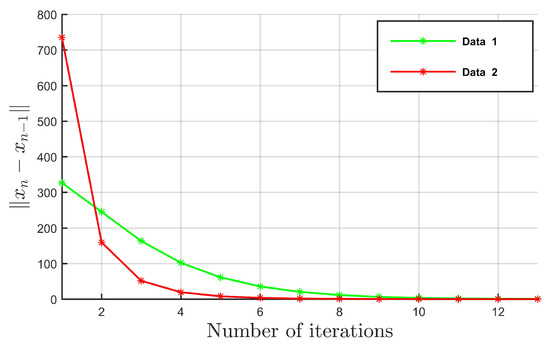
Figure 1. For $N=100$ and $x_0$, $x_1$ are for randomly generated starting points $x_0$ and $x_1$ (the same starting points for Data 1 and Data 2).

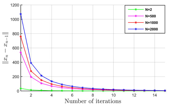
Figure 2. For Data 3 and for randomly generated starting points $x_0$ and $x_1$.

Table 1. For starting points $x_0=10(1,\dots ,1)\in {\mathbb{R}}^N$ and $x_1=10x_0$.

	$\mathit{N}=10$				$\mathit{N}=1200$
	Iter(n)	CPU(s)	$\parallel {\mathit{x}}_{\mathit{n}}\parallel$		Iter(n)	CPU(s)	$\parallel {\mathit{x}}_{\mathit{n}}\parallel$
Data 1	10	0.0165	0.4231		9	0.0182	0.5739
Data 2	9	0.0186	0.4461		8	0.0193	0.3755
Data 3	10	0.0178	0.1356		8	0.0191	0.4524

Data 1. 

${\alpha }_n=\frac{1}{2n+4}$, ${\epsilon }_n=\frac{1}{{(n+2)}^2}$, ${\rho }_n=\frac{n+3}{2n+4}$, ${\lambda }_n=\frac{2}{N+1}$, ${\beta }_n=\frac{n+3}{2n+2}$, ${\theta }_n={\overline{\theta }}_n$.

Data 2. 

${\alpha }_n=\frac{1}{3n^{0.5}+1}$, ${\epsilon }_n=\frac{1}{3n^{1.5}+n}$, ${\rho }_n=\frac{2n^{0.5}-1}{3n^{0.5}+1}$, ${\lambda }_n=\frac{1}{N}$, ${\beta }_n=\frac{1}{2}$, ${\theta }_n={\overline{\theta }}_n$.

Data 3. 

${\alpha }_n=\frac{1}{5n}$, ${\epsilon }_n=\frac{1}{n^3}$, ${\rho }_n=\frac{4n-1}{5n+1}$, ${\lambda }_n=\frac{1}{N+1}$, ${\beta }_n=\frac{10n+91}{11n+110}$, ${\theta }_n={\overline{\theta }}_n$.

The stopping criteria in Table 1 is defined as $\parallel x_n-x_{n-1}\parallel \le {10}^{-3}$.

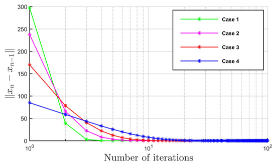
Figure 3 demonstrates the behavior of Algorithm 1 for different parameters ${\rho }_n$ (Case 1: ${\rho }_n=\frac{1}{5n+3}$; Case 2: ${\rho }_n=\frac{2n+2}{5n+3}$; Case 2: ${\rho }_n=\frac{3n+3}{5n+3}$; Case 4: ${\rho }_n=\frac{4n+2}{5n+3}$), where ${\alpha }_n=\frac{1}{5n+3}$, ${\epsilon }_n=\frac{1}{{(5n+3)}^3}$, ${\lambda }_n=\frac{1}{N+1}$, ${\beta }_n=\frac{n+10}{10n+90}$, ${\theta }_n={\overline{\theta }}_n$.

Figure 3. For $N=50$ and starting points $x_0=100(1,\dots ,1)\in {\mathbb{R}}^N$ and $x_1=-50(1,\dots ,1)\in {\mathbb{R}}^N$.

From Figure 1, Figure 2 and Figure 3 and Table 1, it is clear to see that your algorithm depends of the dimension, starting points, and parameters. From Figure 3, we can see that the sequence generated by the algorithm converges faster to the solution of the problem for the choice of ${\rho }_n$, where ρ ($\underset{n\to \infty }{\lim }{\rho }_n=\rho$) is very close to 0.

Example 2.

Consider BVIPO-FM is given by

$$find \overline{x}\in \Omega such that ⟨F(\overline{x}),x-\overline{x}⟩\ge 0,\forall x\in \Omega ,$$

where Ω is the solution set of

$$find x^{\ast }\in C such that f(x^{\ast })=\underset{x\in C}{\min }f(x) and x^{\ast }\in FixU$$

for $H={\mathbb{R}}^N=C$ and F, f, and U are given by

$$F(x)=F(x_1,\dots ,x_N)=(a_1{x}_1+b_1,\dots ,a_N{x}_N+b_N),$$

$$f(x)=\frac{1}{2}{\parallel (I-P_D)2x\parallel }^2,$$

$$Ux=x,$$

where $a_i>0$, $b_i>0$ for all $i\in \{1,\dots ,N\}$ and

$$D=\left\{x\in {\mathbb{R}}^N:\frac{-2\max \{b_i:i=1,\dots ,N\}}{\min \{a_i:i=1,\dots ,N\}}\le x_i\le 0,\forall i\in \{1,\dots ,N\}\right\}.$$

We took $a_i=i$ and $b_i=N+1-i$. Thus, F is β-strongly monotone and κ-Lipschitz continuous on $H={\mathbb{R}}^N$, where $\beta =1$ and $\kappa =N$. The gradient of f is L-Lipschitz continuous on C, where $L=1$ and $\nabla f$ is given by $\nabla f(x)=4x-2P_Q(2x).$ Moreover, $\Omega =\{x\in {\mathbb{R}}^N:-N\le x_i\le 0,\forall i=1,\dots ,N\}$ and

$$SVIP(\Omega ,F)=\left\{\left(-N,\frac{-(N-1)}{2},\frac{-(N-2)}{3},\dots ,\frac{-1}{N}\right)\right\}.$$

Table 2 illustrates the numerical result of our algorithm, solving BVIPO-FM given in this example for different dimensions and different stopping criteria $\frac{\parallel x_n-x_{n-1}\parallel }{\parallel x_1-x_0\parallel }\le TOL$, where the parameters are given in the following: ${\alpha }_n=\frac{1}{5n-1}$, ${\epsilon }_n=\frac{1}{{(5n-1)}^2}$, ${\rho }_n=\frac{1}{5}$, ${\lambda }_n=\frac{1}{N}$, ${\beta }_n=\frac{1}{2}$, ${\theta }_n={\overline{\theta }}_n$.

Table 2. For starting points $x_0=100(1,\dots ,1)\in {\mathbb{R}}^N$ and $x_1=100x_0$.

	TOL = ${10}^{-2}$			TOL = ${10}^{-3}$			TOL = ${10}^{-4}$
	Iter(n)	CPU(s)		Iter(n)	CPU(s)		Iter(n)	CPU(s)
$N=2$	4	0.00345		23	0.3163		107	0.9705
$N=10$	10	0.02217		36	0.4802		116	1.2201
$N=100$	21	0.20681		47	0.9207		149	1.8491

For TOL$={10}^{-5}$, $N=4$, $x_0=(1,2,3,4)$, and $x_1=(5,6,7,8)$, the approximate solution obtained after 319 iterations is

$$x_{319}=(-3.978599508,-1.487950389,-0.641608433,-0.24194702778).$$

6. Conclusions

We have proposed a strongly convergent inertial algorithm for a class of bilevel variational inequality problem over the intersection of the set of common fixed points of finite number of nonexpansive mappings and the set of solution points of the constrained minimization problem of real-valued convex function (BVIPO-FM). The contribution of our result in this paper is twofold. First, it provides effective way of solving BVIPO-FM, where iterative scheme combines inertial term to speed up the convergence of the algorithm. Second, our result can be applied to find a solution to the bilevel variational inequality problem over the solution set of the problem P, where the problem P (the lower level problem) can be converted as a common fixed point of a finite number of nonexpansive mappings.

References

- Deb, K.; Sinha, A. An efficient and accurate solution methodology for bilevel multi-objective programming problems using a hybrid evolutionary-local-search algorithm. Evol. Comput. 2010, 18, 403–449. [Google Scholar] [CrossRef] [PubMed]
- Sabach, S.; Shtern, S. A first order method for solving convex bilevel optimization problems. SIAM J. Optim. 2017, 27, 640–660. [Google Scholar] [CrossRef]
- Shehu, Y.; Vuong, P.T.; Zemkoho, A. An inertial extrapolation method for convex simple bilevel optimization. Optim. Methods Softw. 2019, 1–19. [Google Scholar] [CrossRef]
- Anh, P.K.; Anh, T.V.; Muu, L.D. On bilevel split pseudomonotone variational inequality problems with applications. Acta Math. Vietnam. 2017, 42, 413–429. [Google Scholar] [CrossRef]
- Anh, P.N.; Kim, J.K.; Muu, L.D. An extragradient algorithm for solving bilevel pseudomonotone variational inequalities. J. Glob. Optim. 2012, 52, 627–639. [Google Scholar] [CrossRef]
- Anh, T.T.; Long, L.B.; Anh, T.V. A projection method for bilevel variational inequalities. J. Inequal. Appl. 2014, 1, 205. [Google Scholar] [CrossRef]
- Anh, T.V. A strongly convergent subgradient extragradient-Halpern method for solving a class of bilevel pseudomonotone variational inequalities. Vietnam J. Math. 2017, 45, 317–332. [Google Scholar] [CrossRef]
- Anh, T.V. Linesearch methods for bilevel split pseudomonotone variational inequality problems. Numer. Algorithms 2019, 81, 1067–1087. [Google Scholar] [CrossRef]
- Anh, T.V.; Muu, L.D. A projection-fixed point method for a class of bilevel variational inequalities with split fixed point constraints. Optimization 2016, 65, 1229–1243. [Google Scholar] [CrossRef]
- Chen, J.; Liou, Y.C.; Wen, C.F. Bilevel vector pseudomonotone equilibrium problems: Duality and existence. J. Nonlinear Convex Anal. 2015, 16, 1293–1303. [Google Scholar]
- Van Dinh, B.; Muu, L.D. On penalty and gap function methods for bilevel equilibrium problems. J. Appl. Math. 2011, 2011, 646452. [Google Scholar] [CrossRef]
- Yuying, T.; Van Dinh, B.; Plubtieng, S. Extragradient subgradient methods for solving bilevel equilibrium problems. J. Inequal. Appl. 2018, 2018, 327. [Google Scholar] [CrossRef] [PubMed]
- Bard, J.F. Practical Bilevel Optimization: Algorithms and Spplications; Springer Science & Business Media: Berlin/Heidelberg, Germany, 2013; Volume 30. [Google Scholar]
- Dempe, S. Annotated Bibliography on Bilevel Programming and Mathematical Programs with Equilibrium Constraints. Optimization 2003, 52, 333–359. [Google Scholar] [CrossRef]
- Apostol, R.Y.; Grynenko, A.A.; Semenov, V.V. Iterative algorithms for monotone bilevel variational inequalities. J. Comput. Appl. Math. 2012, 107, 3–14. [Google Scholar]
- Censor, Y.; Gibali, A.; Reich, S. The subgradient extragradient method for solving variational inequalities in Hilbert space. J. Optim. Theory Appl. 2011, 148, 318–335. [Google Scholar] [CrossRef]
- Khanh, P.D. Convergence rate of a modified extragradient method for pseudomonotone variational inequalities. Vietnam J. Math. 2017, 45, 397–408. [Google Scholar] [CrossRef]
- Kalashnikov, V.V.; Kalashinikova, N.I. Solving two-level variational inequality. J. Glob. Optim. 1996, 45, 289–294. [Google Scholar] [CrossRef]
- Calamai, P.H.; Moré, J.J. Projected gradient methods for linearly constrained problems. Math. Program. 1987, 39, 93–116. [Google Scholar] [CrossRef]
- Su, M.; Xu, H.K. Remarks on the gradient-projection algorithm. J. Nonlinear Anal. Optim. 2010, 1, 35–43. [Google Scholar]
- Xu, H.K. Averaged mappings and the gradient-projection algorithm. J. Optim. Theory Appl. 2011, 150, 360–378. [Google Scholar] [CrossRef]
- Polyak, B.T. Some methods of speeding up the convergence of iteration methods. USSR Comput. Math. Math. Phys. 1964, 4, 1–17. [Google Scholar] [CrossRef]
- Lorenz, D.A.; Pock, T. An inertial forward-backward algorithm for monotone inclusions. J. Math. Imaging Vis. 2015, 51, 311–325. [Google Scholar] [CrossRef]
- Ochs, P.; Brox, T.; Pock, T. ipiasco: Inertial proximal algorithm for strongly convex optimization. J. Math. Imaging Vis. 2015, 53, 171–181. [Google Scholar] [CrossRef]
- Bot, R.I.; Csetnek, E.R.; Hendrich, C. Inertial Douglas–Rachford splitting for monotone inclusion problems. Appl. Math. Comput. 2015, 256, 472–487. [Google Scholar]
- Bot, R.I.; Csetnek, E.R. An inertial forward-backward-forward primal-dual splitting algorithm for solving monotone inclusion problems. Numer. Algorithms 2016, 71, 519–540. [Google Scholar] [CrossRef]
- Bot, R.I.; Csetnek, E.R. A hybrid proximal-extragradient algorithm with inertial effects. Numer. Func. Anal. Opt. 2015, 36, 951–963. [Google Scholar] [CrossRef]
- Mann, W.R. Mean value methods in iteration. Proc. Am. Math Soc. 1953, 4, 506–510. [Google Scholar] [CrossRef]
- Byrne, C. A unified treatment of some iterative algorithms in signal processing and image reconstruction. Inverse Probl. 2003, 20, 103. [Google Scholar] [CrossRef]
- Combettes, P.L. Solving monotone inclusions via compositions of nonexpansive averaged operators. Optimization 2004, 53, 475–504. [Google Scholar] [CrossRef]
- Martinez-Yanes, C.; Xu, H.K. Strong convergence of the CQ method for fixed point iteration processes. Nonlinear Anal. 2006, 64, 2400–2411. [Google Scholar] [CrossRef]
- Xu, H.K. Iterative methods for the split feasibility problem in infinite-dimensional Hilbert spaces. Inverse Prob. 2010, 26, 105018. [Google Scholar] [CrossRef]
- Xu, H.K. Iterative algorithms for nonlinear operators. J. Lond. Math. Soc. 2002, 66, 240–256. [Google Scholar] [CrossRef]
- Maingé, P.E. Strong convergence of projected subgradient methods for nonsmooth and nonstrictly convex minimization. Set-Valued Anal. 2008, 16, 899–912. [Google Scholar] [CrossRef]
- Fan, K. A Minimax Inequality and Applications, Inequalities III; Shisha, O., Ed.; Academic Press: New York, NY, USA, 1972. [Google Scholar]
- Combettes, P.L.; Hirstoaga, S.A. Equilibrium programming in Hilbert spaces. J. Nonlinear Convex Anal. 2005, 6, 117–136. [Google Scholar]
- Baillon, J.B.; Haddad, G. Quelques propriétés des opérateurs angle-bornés etn-cycliquement monotones. Isr. J. Math. 1977, 26, 137–150. [Google Scholar] [CrossRef]
- Tang, J.; Chang, S.S.; Yuan, F. A strong convergence theorem for equilibrium problems and split feasibility problems in Hilbert spaces. Fixed Point Theory A 2014, 2014, 36. [Google Scholar] [CrossRef]
© 2019 by the authors. Licensee MDPI, Basel, Switzerland. This article is an open access article distributed under the terms and conditions of the Creative Commons Attribution (CC BY) license (http://creativecommons.org/licenses/by/4.0/).