On Locating and Counting Satellite Components Born along the Stability Circle in the Parameter Space for a Family of Jarratt-Like Iterative Methods

Abstract

This paper is devoted to an analysis on locating and counting satellite components born along the stability circle in the parameter space for a family of Jarratt-like iterative methods. An elementary theory of plane geometric curves is pursued to locate bifurcation points of such satellite components. In addition, the theory of Farey sequence is adopted to count the number of the satellite components as well as to characterize relationships between the bifurcation points. A linear stability theory on local bifurcations is developed based upon a small perturbation about the fixed point of the iterative map with a control parameter. Some properties of fixed and critical points under the Möbius conjugacy map are investigated. Theories and examples on locating and counting bifurcation points of satellite components in the parameter space are presented to analyze the bifurcation behavior underlying the dynamics behind the iterative map.

1. Introduction

A dynamical system can be formulated by any fixed rule describing the time-dependence of an evolving point with its position in the relevant state(phase)-space. It is then best described by a function whose domain and codomain respectively consist of time as an independent variable and state(phase)-space as a dependent variable. The independent variable time can be measured in terms of integers, real or complex numbers. An example of continuous dynamical systems can be seen in differential equations, while other examples of discrete dynamical systems can be seen in difference equations. This analysis will be limited to a discrete dynamical system which is governed by a difference equation in the form of an iterative method: with ${\Psi }_f$ as a fixed point operator [1]

$$x_{n+1}={\Psi }_f\left(x_n\right),forn\in \mathbb{N}\cup \left\{0\right\}.$$

(1)

Such an operator ${\Psi }_f$ can be found in root-finding problems of many fields of applied sciences and has been enhanced by many researchers [2,3,4,5,6,7,8,9] to find better iterative numerical solutions.

The convergence behavior of iterative sequence (1) indeed implies the long-term behavior of discrete dynamical system (1). Hence, taking initial guess $x_0$ as an evolving point, we can trace the long-term behavior of the discrete dynamical system as a sequence of k-fold compositions of ${\Psi }_f$ applied to an initial guess $x_0$:

$$\{x_0,{\Psi }_f\left(x_0\right),{\Psi }_f^2\left(x_0\right),\cdots ,{\Psi }_f^k\left(x_0\right),\cdots ,\},$$

where ${\Psi }_f$ is generally meromorphic. The lemma in Section 1.2.1 of [10] suffices to deal with ${\Psi }_f$ that is a rational function.

Cordero et al. [11] have recently introduced a family of optimal iterative root-finding methods for a system of nonlinear equations $F\left(x\right)=0$ in the following form:

$$\left\{\begin{array}{c}{y}^{\left(n\right)}=x^{\left(n\right)}-\gamma ·{F^{\prime }\left(x^{\left(n\right)}\right)}^{-1}F\left(x^{\left(n\right)}\right),\hfill \\ x^{(n+1)}=x^{\left(n\right)}-H\left(t^{\left(n\right)}\right){F^{\prime }\left(x^{\left(n\right)}\right)}^{-1}F\left(x^{\left(n\right)}\right),n=0,1,\cdots ,\mathrm{with}{t}^{\left(n\right)}={F^{\prime }\left(x^{\left(n\right)}\right)}^{-1}{F}^{\prime }\left(y^{\left(n\right)}\right),\hfill \end{array}\right.$$

(2)

where $\gamma$ is a complex-valued parameter; $F:D\subseteq {\mathbb{C}}^m\to {\mathbb{C}}^m$ has a zero $\alpha \in D$ with $m\in \mathbb{N}$ and is holomorphic [12] in a neighborhood of $\alpha$; $H:X\to X$ is a matrix function with $X={\mathbb{C}}^{m\times m}$ as an $m\times m$ complex matrix satisfying the following hypotheses (i)–(iii):

(i)

$H^{\prime }\left(u\right)\left(v\right)=h_{1}uv$ with $H^{\prime }$ as the first derivative of H such that $H^{\prime }:X\to \mathcal{L}\left(X\right),$

(ii)

$H^{″}(u,v)\left(w\right)=h_{2}uvw$ with $H^{″}$ as the second derivative of H such that $H^{″}:X^{\prime 2}\to \mathcal{L}\left(X\right),$

(iii)

$H^{‴}(u,v,w)\left(s\right)=h_{3}uvws$ with $H^{‴}$ as the third derivative of H such that $H^{‴}:X^{\prime 3}\to \mathcal{L}\left(X\right)$,

where $\mathcal{L}\left(X\right)$ denotes the space of linear mappings from $X\to X$ and $h_1,h_2,h_3\in \mathbb{C}$.

Then, we have the following variant of Theorem 3 presented from Cordero et al. [11]:

Theorem 1.

Let $\gamma =2/3,F$ and H be introduced in Equation (2) with $H\left(I\right)=I,h_1=-3/4,h_2=9/4$ and $|h_3|<\infty$. Then, iterative numerical scheme (2) converges to the root α of F, starting from a given initial guess $x^{\left(0\right)}$ sufficiently close to α, with the following error equation:

$$e_{n+1}=\left((5+\frac{38}{81}{h}_3)C_2^3-C_2{C}_3+\frac{C_4}{9}\right)e_n^4+O\left(e_n^5\right),$$

where $C_j=\frac{1}{j!}{F^{\prime }\left(\alpha \right)}^{-1}F\left(\alpha \right),j=2,3,\cdots$ and $e_n=x^{\left(n\right)}-\alpha$.

Applications of the above theorem cover a number of existing studies introduced in [11] and references cited therein. For $m=1$, by considering the one-point compactification of $\mathbb{C}$, namely, the Riemann sphere $\overline{\mathbb{C}}=\mathbb{C}\cup \{\infty \}$, Cordero et al. [11] have pursued the complex dynamics on $\overline{\mathbb{C}}$ for Jarratt-like uniparametric iterative map (2), with

$$H\left(t\right)=1-\frac{3}{4}(t-1)+\frac{9}{8}{(t-1)}^2+\frac{1}{6}\lambda {(t-1)}^3\mathrm{for}\mathrm{parameter}\lambda =h_3,$$

(3)

for periodic points via Möbius conjugacy [13] map $M\left(z\right)=\frac{z-a}{z-b},(a\ne b)$ applied to a quadratic polynomial $(z-a)(z-b)$. Although they included an analysis of the $\lambda$-parameter space, our primary aim of this paper is to pursue a somewhat advanced study of the $\lambda$-parameter space where bifurcation behavior along the stability circle needs to be extensively analyzed.

The remaining part of this paper is devoted to the development of further properties in additional five sections. Described in Section 2 are preliminary studies on long-term behavior of a dynamical system via conjugacy defined on $\overline{\mathbb{C}}$. Section 3 fully discusses a linear stability theory based on the analysis of a small perturbation about the fixed point of the iterative map (2) under the Möbius conjugacy and classifies the local bifurcations into three types according to the location of the spectral radius of the conjugated iterative map along the unit circle. In Section 4, we describe some properties of the fixed and critical points related to the dynamics under the Möbius conjugacy map. Section 5 investigates a long-term dynamical behavior of the conjugated iterative map. Parameter spaces along with dynamical planes are defined and extensively explored with a number of self-explanatory illustrative figures. In addition, we develop a theory on tracking down bifurcation points budding from another component [14] in the parameter space from a viewpoint of plane geometry. Finally, in Section 6, we draw an overall conclusion and briefly state the future work.

2. Preliminary Studies

For ease of discussion of two dynamical systems F and G, one needs to perceive the notion of conjugacy [15,16], follow Theorem 2.1 of [16] describing the invariances of topological and diffeomorphic conjugacies, and remark on the preservation of the dynamical behavior between two n-fold composite dynamical systems $F^n$ and $G^n$ under topological conjugacy with $F^n=h\circ G^n\circ h^{-1}$ for any integer n.

The following lemma is a variant of the well-known Banach fixed-point theorem or contraction mapping principle [17].

Lemma 1.

Let $\Omega \subset \mathbb{C}$ and $f:\Omega \to \Omega$ be analytic. Furthermore, let f have a fixed point $\xi \in \Omega$ with $|f^{\prime }\left(\xi \right)|<1$. Then, f has a unique fixed point ξ and the sequence ${\{z_{n+1}=f\left(z_n\right)\}}_0^{\infty }$ converges to ξ, provided that any $z_0\in \Omega$ is given.

In Lemma 1, $z_0$ can be chosen as a critical point $z^{*}$ of f, due to the fact that $f^{\prime }\left(z^{*}\right)=0$ implies $z^{*}\in \Omega$. The result of Lemma 1 with $z_0=z^{*}$ yields the following corollary.

Corollary 1.

Let ξ be the fixed point described in Lemma 1. Then, every critical orbit (which is an orbit of a critical point) of f tends to ξ.

Remark 1.

Corollary 1 provides a background for the definition of the parameter space to be discussed in Section 5. In fact, an orbit of any point in a small neighborhood of the fixed point ξ tends to ξ according to Proposition 4.4 of [18], which constitutes a basis for the definition of the dynamical plane in Section 5.

The following definition [19,20,21] plays a role in describing the qualitative behavior of a dynamical system.

Definition 1.

Let $z_0$ be in the domain of f. The orbit of $z_0$ is defined to be the sequence ${\left\{f^k\left(z_0\right)\right\}}_{k=0}^{\infty }$ with $f^k$ as the k-fold composite map of f. Then, we say the following:

(a) 

$z_0$ has period k (or is a period-k point ) if $f^k\left(z_0\right)=z_0$, with all distinct $z_0,f\left(z_0\right),f^2\left(z_0\right),\cdots ,f^{k-1}\left(z_0\right)$. If $k=1$, then $z_0$ is called a fixed point.

(b) 

If $z_0$ is a period-k point (or k-periodic point), then the orbit of $z_0$ is called a k-periodic orbit (or k-cycle).

(c) 

If $z_0$ is a point some iterate of which is periodic, i.e., if there exists an integer $1\le \ell \le k-2$ satisfying $f^k\left(z_0\right)=f^{k-\ell }\left(z_0\right)$, then $z_0$ is called an eventually periodic (or a pre-periodic) point.

(d) 

If the the orbit of $z_0$ contains a subsequence converging to to a stable periodic point, then $z_0$ is called an asymptotically periodic point.

(e) 

If $z_0$ is not of types (a),(c),(d), then $z_0$ is called an aperiodic (or a non-periodic) point. The orbit of such $z_0$ is said to be “non-periodic, stochastic or chaotic”.

3. Linear Stability Theory and Local Bifurcations

Consider a discrete dynamical system $\mathcal{F}:{\mathbb{C}}^m\times \mathbb{C}\to {\mathbb{C}}^m$ with $m\in \mathbb{N}$ defined by

$$z_{n+1}=\mathcal{F}(z_n,\lambda ),n\in \mathbb{N}\cup \left\{0\right\},$$

(4)

where $\lambda \in \mathbb{C}$ is a control parameter and $z_0\in {\mathbb{C}}^m$ is given. Assuming $\xi \in {\mathbb{C}}^m$ is a fixed point of $\mathcal{F}$, we take a small perturbation about $\xi$ by writing

$$z_n=\xi +{\delta }_n,$$

(5)

where the initial perturbation ${\delta }_0\ne 0$ is arbitrary. For a given $\lambda$, expanding Equation (4) about $\xi$ up to the first-order term in ${\delta }_n$ yields:

$$\xi +{\delta }_{n+1}=\mathcal{F}(\xi +{\delta }_n,\lambda )=\mathcal{F}(\xi ,\lambda )+\mathit{S}{\delta }_n+O\left(\right|{\delta }_n{|}^2),$$

(6)

with $\mathit{S}=\mathit{S}(\xi ,\lambda )$ as an $m\times m$ Jacobian matrix evaluated at $\xi$. As a consequence, we are ready to discuss the linear stability about the fixed point by considering

$${\delta }_{n+1}=\mathit{S}{\delta }_n.$$

(7)

We transform Equation (7) by means of an $m\times m$ nonsingular matrix P to obtain

$$b_{n+1}=\mathit{J}{b}_n,$$

(8)

where $b_n={\mathit{P}}^{-1}{\delta }_n$, and $J={\mathit{P}}^{-1}\mathit{S}\mathit{P}$ is the Jordan canonical form [22] of S with k Jordan blocks ${\mathit{J}}_1,{\mathit{J}}_2,\cdots ,{\mathit{J}}_k$. A typical ${\mathit{J}}_i$ is given by an $r_i\times r_i$ upper triangular matrix with ${\omega }_i$’s as all diagonal entries and 1’s as all super-diagonal entries as shown below:

$${\mathit{J}}_i=\left(\begin{array}{ccccc}{\omega }_i& 1& 0& \cdots & 0\\ 0& {\omega }_i& 1& \ddots & ⋮\\ ⋮& \ddots & \ddots & \ddots & 0\\ 0& \cdots & 0& {\omega }_i& 1\\ 0& \cdots & \cdots & 0& {\omega }_i\end{array}\right),$$

where ${\omega }_i$ is an eigenvalue of S. Without loss of generality, let ${\mathit{J}}_i$ be chosen such that $|{\omega }_i|=\rho \left(\mathit{S}\right)$, which is the spectral radius of S. For simplicity, we denote ${\mathit{J}}_i$ by $\tilde{\mathit{J}}$, ${\omega }_i$ by $\omega$ and $r_i$ by r. The limit behavior of the perturbation ${\delta }_n=\mathit{P}{b}_n$ will be best described by analyzing a subsystem

$${\tilde{b}}_{n+1}=\tilde{\mathit{J}}{\tilde{b}}_n={\tilde{\mathit{J}}}^n{\tilde{b}}_0,$$

(9)

where ${\tilde{b}}_n\in {\mathbb{C}}^r$ consists of the corresponding r components of $b_n$ related with $\tilde{\mathit{J}}$. Note that, by induction on $n\in \mathbb{N}$, ${\tilde{\mathit{J}}}^n$ is given by

$${\tilde{\mathit{J}}}^n=\left(\begin{array}{ccccc}{\omega }^n& \left(\genfrac{}{}{0pt}{}{n}{1}\right){\omega }^{n-1}& \left(\genfrac{}{}{0pt}{}{n}{2}\right){\omega }^{n-2}& \cdots & \left(\genfrac{}{}{0pt}{}{n}{r-1}\right){\omega }^{n-r+1}\\ 0& {\omega }^n& \left(\genfrac{}{}{0pt}{}{n}{1}\right){\omega }^{n-1}& \cdots & \left(\genfrac{}{}{0pt}{}{n}{r-2}\right){\omega }^{n-r+2}\\ ⋮& \ddots & \ddots & \ddots & ⋮\\ ⋮& \ddots & \ddots & {\omega }^n& \left(\genfrac{}{}{0pt}{}{n}{1}\right){\omega }^{n-1}\\ 0& \cdots & \cdots & 0& {\omega }^n\end{array}\right).$$

(10)

If $r=1$ in Equation (10), i.e., all eigenvalues of S are simple, then, based on the component-wise expressions, we easily obtain the following lemma:

Lemma 2.

(i)

${lim}_{n\to \infty }{\delta }_n=0$ if and only if $\rho \left(\mathit{S}\right)<1$.

(ii)

$|{lim}_{n\to \infty }{\delta }_n|=\infty$ if and only if $\rho \left(\mathit{S}\right)>1$.

(iii)

$0<|{lim}_{n\to \infty }{\delta }_n|\le M$ for some finite $M>0$ if and only if $\rho \left(\mathit{S}\right)=1$.

If $r\ge 2$ in Equation (10), i.e., some eigenvalues of S are multiple, and then we obtain:

Lemma 3.

(i)

${lim}_{n\to \infty }{\delta }_n=0$ if and only if $\rho \left(\mathit{S}\right)<1$.

(ii)

$|{lim}_{n\to \infty }{\delta }_n|=\infty$ if and only if $\rho \left(\mathit{S}\right)\ge 1$.

Proof. 

(i) After close inspection of upper off-diagonal entries in Equation (10), we find ${lim}_{n\to \infty }\left(\genfrac{}{}{0pt}{}{n}{j}\right){\left|\omega \right|}^{n-j}={lim}_{n\to \infty }\frac{n(n-1)(n-2)\cdots (n-j+1)}{{j!\left|\omega \right|}^{j-n}}={lim}_{n\to \infty }\frac{n(n-1)(n-2)\cdots (n-j+1)}{j!e^{(j-n)ln\left|\omega \right|}}=0$ for $1\le j\le r-1$ if and only if $\left|\omega \right|<1$ by applying L’Hospitals’s rule j times. Hence, all upper off-diagonal entries vanish as $n\to \infty$ if and only if $\left|\omega \right|<1$. (ii) Similarly, we find ${lim}_{n\to \infty }\left(\genfrac{}{}{0pt}{}{n}{j}\right){\left|\omega \right|}^{n-j}=\infty$ for $1\le j\le r-1$ if and only if $\left|\omega \right|\ge 1$. □

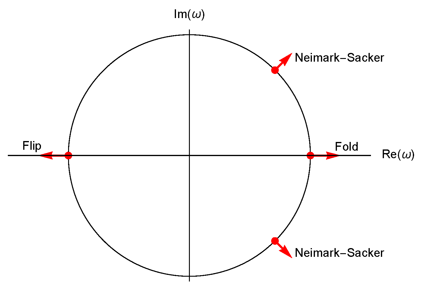
Remark 2.

When all eigenvalues of S are simple, according to Lemma 2, the fixed point behavior or long-term orbit behavior of the iterative map $\mathcal{F}$ is stable if and only if $\rho \left(\mathit{S}\right)<1$ (modulus of all eigenvalues of $\mathit{S}<1$), and unstable if and only if $\rho \left(\mathit{S}\right)>1$ (modulus of some eigenvalues of $\mathit{S}>1$) from a viewpoint of the linear stability. According to the Bolzano–Weierstrass Theorem [14], the result (iii) of Lemma 2 indicates that there exists a convergent subsequence of $\left\{{\delta }_n\right\}$, which will induce k-periodic orbits of $\mathcal{F}$ as well as its non-periodic bounded orbits, if and only if $\rho \left(\mathit{S}\right)=1$.

Since $\rho \left(\mathit{S}\right)$ around the unit circle plays a significant role in stability analysis, we had better designate the unit circle as the stability unit circle shown in Figure 1 for further analysis.

Consequently, the geometrical properties in the parameter space when $\rho \left(\mathit{S}\right)=1$ would play key roles in analyzing the long-term orbit behavior of $\mathcal{F}$. Such a long-term orbit behavior will often experience an abrupt qualitative change when an eigenvalue $\omega$ (or Floquet multiplier [23]) of S with the maximum modulus crosses a certain location ${\omega }^{*}$ of the stability unit circle. This kind of qualitative change in the behavior of a dynamical system is called a bifurcation. We classify such bifurcations [24] in the space of control parameters into three types according to the location of ${\omega }^{*}$ along the stability unit circle as follows:

(1)

The (cyclic) fold(saddle-node) bifurcation occurs when ${\omega }^{*}=1$.

(2)

The flip(period-doubling) bifurcation occurs when ${\omega }^{*}=-1$.

(3)

The Neimark–Sacker(secondary Hopf) bifurcation occurs when ${\omega }^{*}=e^{i\theta }$, purely complex, with $\theta \ne \pi ,0<\theta <2\pi$.

The location of the control parameter in the parameter space where a qualitative change in the behavior of a dynamical system occurs is called a bifurcation point. To locate such a bifurcation point, after solving the relation $\left|\omega \right|=\rho \left(\mathit{S}\right(\xi ,\lambda )=1$ for $\lambda$ in terms of $\omega$ exactly or numerically, we can trace the control parameter $\lambda$ as $\omega$ varies along the stability unit circle. As a result, the bifurcation point ${\lambda }^{*}$ in the parameter space can be given by $\lambda \left({\omega }^{*}\right)$ based on the types of bifurcation mentioned above.

4. Fixed and Critical Points under the Möbius Conjugacy Map

For iterative map (2) with $m=1$ and $H\left(t\right)$ given by Equation (3), we will discuss some properties of fixed and critical points under the Möbius conjugacy map, as $\lambda$ varies in the finite complex plane. To effectively treat a one-dimensional iterative map, we conveniently denote $x^{\left(n\right)}=x_n$ for $n\in \mathbb{N}\cup \left\{0\right\}$.

Let ${\Psi }_f$ be defined by $x_{n+1}={\Psi }_f\left(x_n\right)$ in Equation (2) and be conjugate to a map J through a diffeomorphic Möbius conjugacy map $M\left(z\right)$ as introduced in Section 1. For ease of analysis, we consider $f\left(z\right)=(z-a)(z-b)$ as a prototype quadratic polynomial and find that the resulting J will generally take the form dependent on $a,b$ and $\lambda$. Very favorably, $M\left(z\right)$ with $f\left(z\right)=(z-a)(z-b)$ leads us to:

$$J(z;\lambda )=\frac{z^4(405+32\lambda +1134z+1134z^2+486z^3+81z^4)}{81+486z+1134z^2+1134z^3+z^4(405+32\lambda )},$$

(11)

which is free of a and b.

We now find the derivative of J from Equation (11) given by:

$$J^{\prime }(z;\lambda )=\frac{324z^3{(z+1)}^{6}Q(z;\lambda )}{q{\left(z\right)}^2},$$

(12)

where $Q(z;\lambda )=405+32\lambda +z(810-48\lambda )+z^2(405+32\lambda )$ and $q\left(z\right)=81+486z+1134z^2+1134z^3+z^4(405+32\lambda )$.

With our first glance of Equation (12), we find that $z=-1$ is a free critical points [25] for any $\lambda \in \mathbb{C}$. Other free critical points may be found from the roots of $Q(z;\lambda )$ as a function of $\lambda$.

Useful properties of J and $J^{\prime }$ regarding the strange fixed points [25] and free critical points can be derived in the similar manner as done in Sections 3.1 and 3.2 of [16]. The important consequences of these properties lead us to the following proposition:

Proposition 1.

(a)

If $\xi \in \overline{\mathbb{C}}$ is any fixed point of J, then so is $\frac{1}{\xi }$.

(b)

If $\zeta \in \overline{\mathbb{C}}$ is any critical point of J, then so is $\frac{1}{\zeta }$.

(c)

$J(\frac{1}{z};\lambda )=\frac{1}{J(z;\lambda )}$ holds for any $\lambda \in \mathbb{C}$ and any $z\in \overline{\mathbb{C}}$.

(d)

$J^{\prime }(\xi ;\lambda )=J^{\prime }(\frac{1}{\xi };\lambda )forany\lambda \in \mathbb{C}$ and any fixed point $\xi \in \overline{\mathbb{C}}$ of J.

The underlying dynamics behind iterative map (11) will be initiated by investigating the fixed points of J and their stability. Fixed points of J can bound from the roots of $J(z;\lambda )-z$:

$$J(z;\lambda )-z=\frac{z(z-1)·T(z;\lambda )}{q\left(z\right)},$$

(13)

where $T(z;\lambda )=81+567z+1701z^2+z^3(2430-32\lambda )+1701z^4+567z^5+81z^6$.

Clearly, $z=1$ is a strange fixed point which may give us an appealing impact on the relevant dynamics. To locate other strange fixed points dependent on $\lambda$, we seek the roots z of $T(z;\lambda )=0$ in Equation (13) for given values of $\lambda$. In view of Proposition 1(a), the strange fixed points of $J(z;\lambda )$ are found by solving $T(z;\lambda )=\prod {}_{i=1}^3(z^2+c_{i}z+1)=0$, i.e., $z=-\frac{1}{2}\left(c_i+\sqrt{c_i^2-4}\right)$ where $c_i,(1\le i\le 3)$ are the three roots of the relation $16(2\lambda -81)+1698c-567c^2+c^3=0$.

In view of Equation (12), we are able to describe the stability of the strange fixed point $z\left(\lambda \right)=1$ using $\lambda$-values in the following theorem whose proof is the similar to that of Theorem 3.5 from [16].

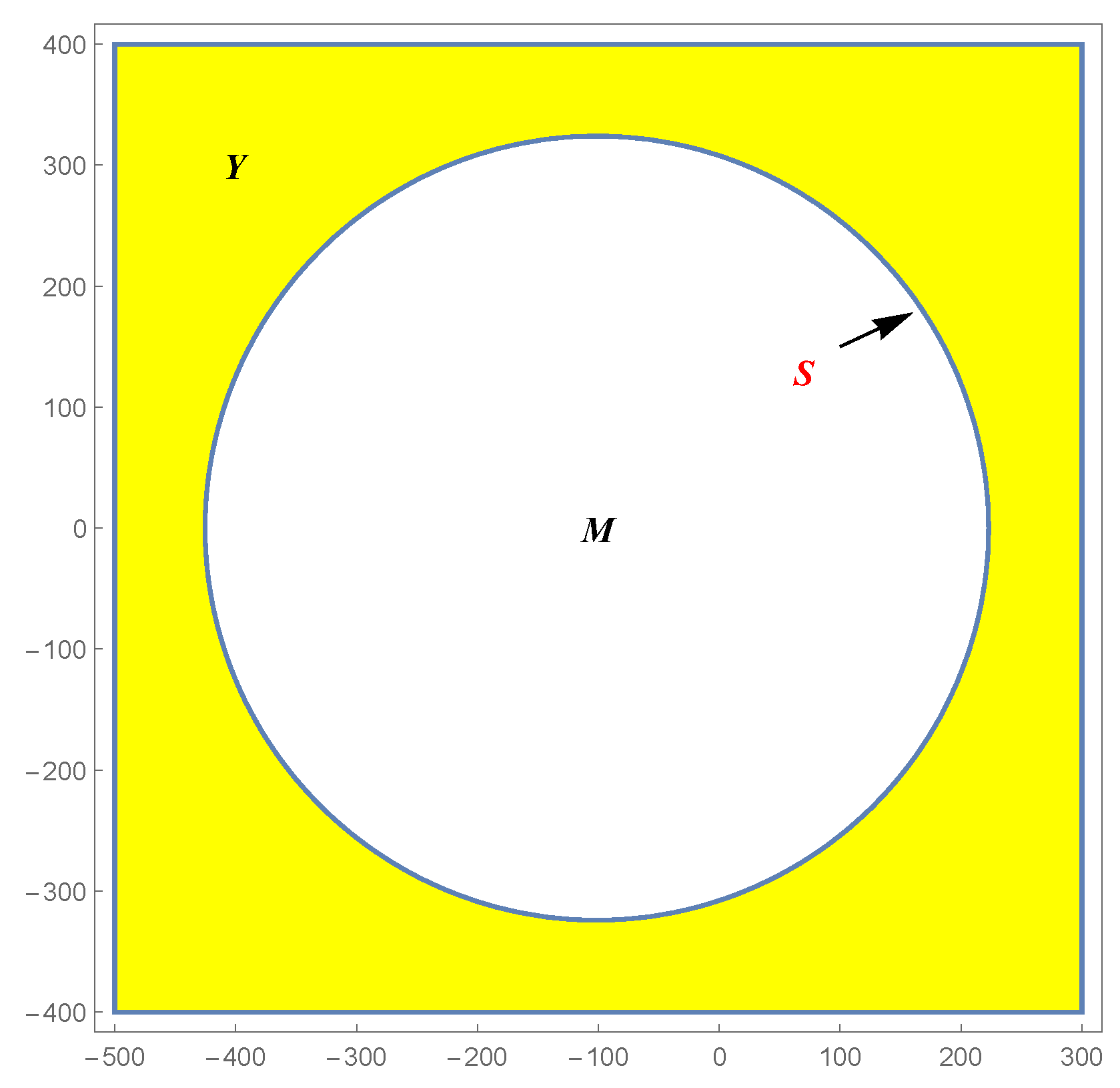
Theorem 2.

Let us define $\mathit{Y}=\{\lambda \in \mathbb{C}:|\lambda +\frac{405}{4}|>324\}$, $\mathit{S}=\{\lambda \in \mathbb{C}:|\lambda +\frac{405}{4}|=324\}$ and $M=\{\lambda \in \mathbb{C}:|\lambda +\frac{405}{4}|<324\}$. Then, the strange fixed point $z\left(\lambda \right)=1$ becomes attractive, parabolic, and repulsive, respectively, whenever $\lambda \in \mathit{Y}$, $\lambda \in \mathit{S}$, and $\lambda \in \mathit{M}$.

Remark 3.

Figure 2 displays Y, S, and M. It is better to call S the stability circle since the fixed point $z\left(\lambda \right)=1$ with λ in a neighborhood of S becomes either repulsive or attractive.

5. Bifurcation in the Parameter Space

Our further investigation on the complex dynamics of conjugated map $J(z;\lambda )$ given by Equation (11) is essentially limited to the analysis of long-term behavior of $J(z;\lambda )$. A useful task is preferably to use a free critical point z and generate its orbit under the action of $J(z;\lambda )$, which will induce attracting periodic orbits for each given $\lambda$ according to Corollary 1. The orbit behavior of two critical points z and $\frac{1}{z}$ of J is best described in Proposition 1(c) and Remark 4.

Corollary 2.

Let $q\in \mathbb{N}$ be given. If $z\in \overline{\mathbb{C}}$ is a q-periodic point of J, then so is $\frac{1}{z}$.

Proof. 

With the help of Proposition 1(c) and fixed point invariance property [16] under topological conjugacy for q-fold composition of J with $h\left(z\right)=\frac{1}{z}$, we easily find that $J^q(\frac{1}{z};\lambda )=\frac{1}{J^q(z;\lambda )}=\frac{1}{z}$ for any given $\lambda \in \mathbb{C}$. □

Proposition 2.

Let $\xi \left(\lambda \right)$ be a fixed point of $J(z;\lambda )$ found from $T(z;\lambda )=0$ in Equation (13). Let ${\zeta }_1\left(\lambda \right)$ and ${\zeta }_2\left(\lambda \right)=\frac{1}{{\zeta }_1\left(\lambda \right)}$ be two critical points of $J(z;\lambda )$ found from $Q(z;\lambda )=0$ in Equation (12). Suppose that the orbit of critical point ${\zeta }_1$ approaches a q-periodic point ξ of J, i.e., $J^q(\xi ;\lambda )=\xi$ in the long run for a given $\lambda \in \mathbb{C}$ and $q\in \mathbb{N}$. Then, the orbit of ${\zeta }_2$ approaches a q-periodic point $\frac{1}{\xi }$ of $J(z;\lambda )$.

Proof. 

$$\xi \left(\lambda \right)=\underset{n\to \infty }{lim}{J}^n({\zeta }_1;\lambda )=\underset{k\to \infty }{lim}{J}^{pk+q}({\zeta }_1;\lambda )=J^q\circ (\underset{k\to \infty }{lim}{J}^{pk}({\zeta }_1;\lambda )=J^q(\xi \left(\lambda \right);\lambda ),$$

(14)

after writing out $n=pk+q$ for any $p\in \mathbb{N}$ with $q\in \{0,1,2,\cdots ,p-1\}$. In view of Proposition 1(c) and Equation (14), we find:

${\displaystyle \underset{n\to \infty }{lim}{J}^n({\zeta }_2;\lambda )=\underset{n\to \infty }{lim}{J}^n(\frac{1}{{\zeta }_1};\lambda )=\frac{1}{{lim}_{n\to \infty }{J}^n({\zeta }_1;\lambda )}=\frac{1}{J^q(\xi ;\lambda )}=\frac{1}{\xi }=J^q(\frac{1}{\xi };\lambda ).}$ □

Remark 4.

In view of Proposition 2, the orbit of ${\zeta }_2$ behaves in quite the same way as the other ${\zeta }_1$ does.

By consulting Section 4.1 of [16], we now reintroduce the notions of the parameter space $\mathcal{P}$ and dynamical plane $\mathcal{D}$ to effectively display the iteration dynamics of J as follows:

$$\begin{array}{c}\mathcal{P}=\{\lambda \in \mathbb{C}:\text{an orbit of a free critical point}z\text{tends to a number}{\sigma }_p\in \overline{\mathbb{C}}\text{under the action of}J(z;\lambda )\},\hfill \\ \mathcal{D}=\{z\in \mathbb{C}:\text{an orbit of z for a given}z\text{for a given}\lambda \in \mathcal{P}\text{tends to a number}{\sigma }_d\in \overline{\mathbb{C}}\text{under the action of}J(z;\lambda )\}.\hfill \end{array}$$

In view of Equation (13), the possible fixed points are given by $0,1,\infty$ and $\xi \left(\lambda \right)$. When ${\sigma }_p,{\sigma }_d\in \{0,1,\infty ,\xi \left(\lambda \right)\}$, there may exist a q-periodic point in the orbit for $q\in \mathbb{N}\cup \left\{0\right\}$. If $q=0$, then the orbit is non-periodic but bounded.

Thanks to the basic properties of the dynamical plane $\mathcal{D}$ consisting of a union of attractor basins, extensively studied in [11], we in this paper only investigate some interesting properties of the parameter plane $\mathcal{P}$. According to Remark 4, we consider only one branch of the critical points ${\zeta }_1$ for its typical orbit behavior.

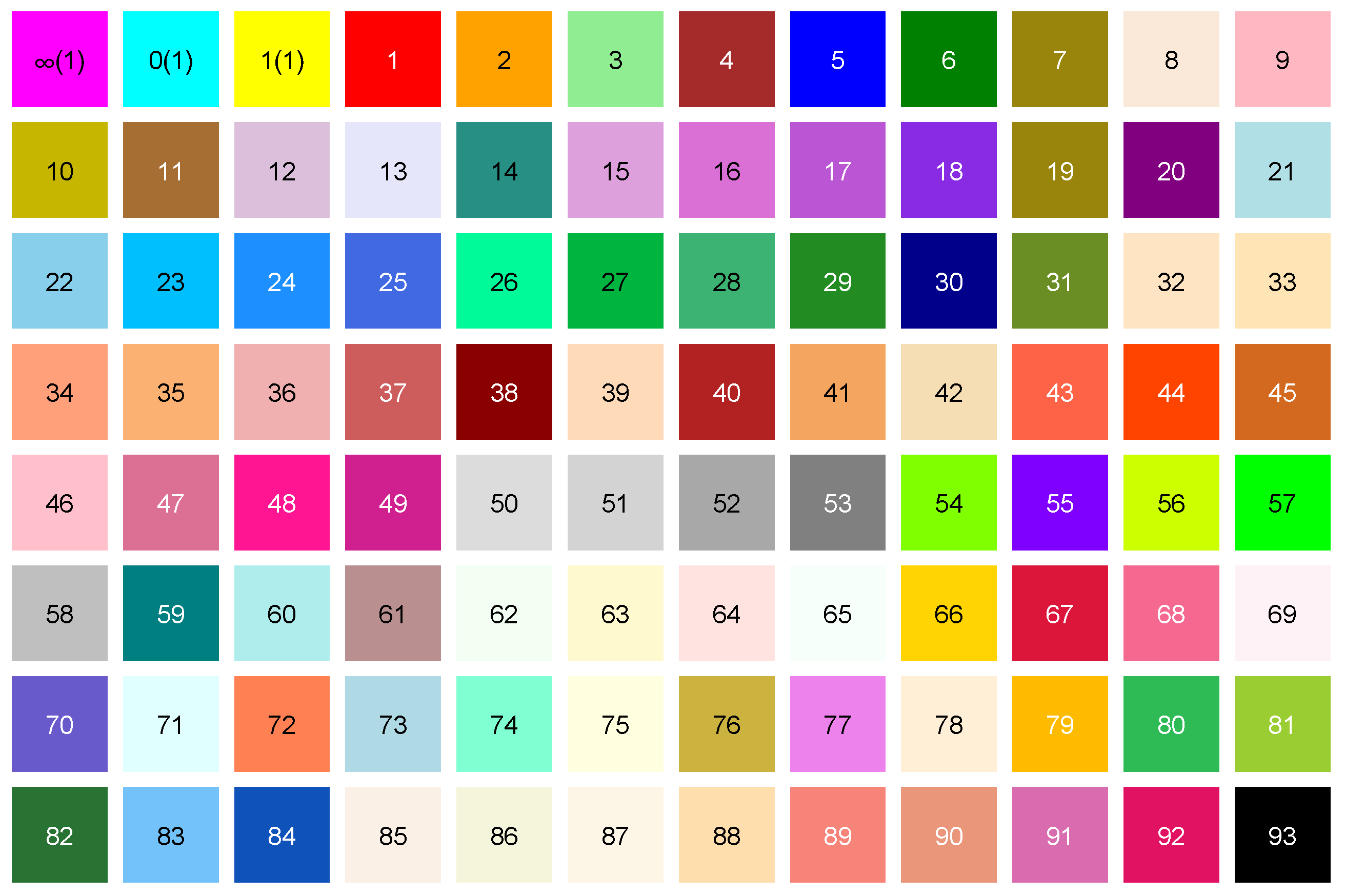
In Figure 4, a parameter space $\mathcal{P}$ associated with free critical points ${\zeta }_1\left(\lambda \right)$ is illustrated. If a q-periodic orbit is generated under the action of $J({\zeta }_1;\lambda )$ for $\lambda \in \mathcal{P}$, then $\lambda$ is painted in color $c_q$ assigned by

Table 1. Coloring scheme for a q-periodic orbit with $q\in \mathbb{N}\cup \left\{0\right\}$.

q	${\mathit{C}}_{\mathit{q}}$
1	$\stackrel{C_1(\mathrm{fixed}\mathrm{point}\infty )}{\mathrm{magenta}}$	$\stackrel{C_1\left(\mathrm{fixed}\mathrm{point}0\right)}{\mathrm{cyan}}$	$\stackrel{C_1\left(\mathrm{fixed}\mathrm{point}1\right)}{\mathrm{yellow}}$	$\stackrel{C_1\left(\mathrm{other}\mathrm{strange}\mathrm{fixed}\mathrm{point}\right)}{\mathrm{red}}$
	$\stackrel{C_2}{\mathrm{orange}}$	$\stackrel{C_3}{\mathrm{light}\mathrm{green}}$	$\stackrel{C_4}{\mathrm{brown}}$	$\stackrel{C_5}{\mathrm{blue}}$	$\stackrel{C_6}{\mathrm{green}}$	$\stackrel{C_7}{\mathrm{dark}\mathrm{yellow}}$	$\stackrel{C_8}{\mathrm{antique}\mathrm{white}}$
	$\stackrel{C_9}{\mathrm{light}\mathrm{pink}}$	$\stackrel{C_{10}}{\mathrm{khaki}}$	$\stackrel{C_{11}}{\mathrm{melon}}$	$\stackrel{C_{12}}{\mathrm{thistle}}$	$\stackrel{C_{13}}{\mathrm{lavender}}$	$\stackrel{C_{14}}{\mathrm{turquoise}}$	$\stackrel{C_{15}}{\mathrm{plum}}$
	$\stackrel{C_{16}}{\mathrm{orchid}}$	$\stackrel{C_{17}}{\mathrm{medium}\mathrm{orchid}}$	$\stackrel{C_{18}}{\mathrm{blue}\mathrm{violet}}$	$\stackrel{C_{19}}{\mathrm{dark}\mathrm{orchid}}$	$\stackrel{C_{20}}{\mathrm{purple}}$	$\stackrel{C_{21}}{\mathrm{powder}\mathrm{blue}}$	$\stackrel{C_{22}}{\mathrm{sky}\mathrm{blue}}$
	$\stackrel{C_{23}}{\mathrm{deep}\mathrm{sky}\mathrm{blue}}$	$\stackrel{C_{24}}{\mathrm{dodger}\mathrm{blue}}$	$\stackrel{C_{25}}{\mathrm{royal}\mathrm{blue}}$	$\stackrel{C_{26}}{\mathrm{medium}\mathrm{spring}\mathrm{green}}$	$\stackrel{C_{27}}{\mathrm{apple}\mathrm{green}}$	$\stackrel{C_{28}}{\mathrm{medium}\mathrm{sea}\mathrm{green}}$	$\stackrel{C_{29}}{\mathrm{forest}\mathrm{green}}$
	$\stackrel{C_{30}}{\mathrm{dark}\mathrm{blue}}$	$\stackrel{C_{31}}{\mathrm{olive}\mathrm{drab}}$	$\stackrel{C_{32}}{\mathrm{bisque}}$	$\stackrel{C_{33}}{\mathrm{moccasin}}$	$\stackrel{C_{34}}{\mathrm{light}\mathrm{salmon}}$	$\stackrel{C_{35}}{\mathrm{salmon}}$	$\stackrel{C_{36}}{\mathrm{light}\mathrm{coral}}$
	$\stackrel{C_{37}}{\mathrm{Indian}\mathrm{red}}$	$\stackrel{C_{38}}{\mathrm{dark}\mathrm{red}}$	$\stackrel{C_{39}}{\mathrm{peach}\mathrm{puff}}$	$\stackrel{C_{40}}{\mathrm{fire}\mathrm{brick}}$	$\stackrel{C_{41}}{\mathrm{sandy}\mathrm{brown}}$	$\stackrel{C_{42}}{\mathrm{wheat}}$	$\stackrel{C_{43}}{\mathrm{tomato}}$
$2\le q\le 92$	$\stackrel{C_{44}}{\mathrm{orange}\mathrm{red}}$	$\stackrel{C_{45}}{\mathrm{chocolate}}$	$\stackrel{C_{46}}{\mathrm{pink}}$	$\stackrel{C_{47}}{\mathrm{pale}\mathrm{violet}\mathrm{red}}$	$\stackrel{C_{48}}{\mathrm{deep}\mathrm{pink}}$	$\stackrel{C_{49}}{\mathrm{violet}\mathrm{red}}$	$\stackrel{C_{50}}{\mathrm{gainsboro}}$
	$\stackrel{C_{51}}{\mathrm{light}\mathrm{gray}}$	$\stackrel{C_{52}}{\mathrm{dark}\mathrm{gray}}$	$\stackrel{C_{53}}{\mathrm{gray}}$	$\stackrel{C_{54}}{\mathrm{charteruse}}$	$\stackrel{C_{55}}{\mathrm{electric}\mathrm{indigo}}$	$\stackrel{C_{56}}{\mathrm{electric}\mathrm{lime}}$	$\stackrel{C_{57}}{\mathrm{lime}}$
	$\stackrel{C_{58}}{\mathrm{silver}}$	$\stackrel{C_{59}}{\mathrm{teal}}$	$\stackrel{C_{60}}{\mathrm{pale}\mathrm{turquoise}}$	$\stackrel{C_{61}}{\mathrm{rosy}\mathrm{brown}}$	$\stackrel{C_{62}}{\mathrm{honeydew}}$	$\stackrel{C_{63}}{\mathrm{lemon}\mathrm{chiffon}}$	$\stackrel{C_{64}}{\mathrm{misty}\mathrm{rose}}$
	$\stackrel{C_{65}}{\mathrm{mint}\mathrm{cream}}$	$\stackrel{C_{66}}{\mathrm{gold}}$	$\stackrel{C_{67}}{\mathrm{crimson}}$	$\stackrel{C_{68}}{\mathrm{light}\mathrm{crimson}}$	$\stackrel{C_{69}}{\mathrm{lavender}\mathrm{blush}}$	$\stackrel{C_{70}}{\mathrm{slate}\mathrm{blue}}$	$\stackrel{C_{71}}{\mathrm{light}\mathrm{cyan}}$
	$\stackrel{C_{72}}{\mathrm{coral}}$	$\stackrel{C_{73}}{\mathrm{light}\mathrm{blue}}$	$\stackrel{C_{74}}{\mathrm{aquamarine}}$	$\stackrel{C_{75}}{\mathrm{light}\mathrm{yellow}}$	$\stackrel{C_{76}}{\mathrm{peru}}$	$\stackrel{C_{77}}{\mathrm{violet}}$	$\stackrel{C_{78}}{\mathrm{papaya}\mathrm{whip}}$
	$\stackrel{C_{79}}{\mathrm{dark}\mathrm{orange}}$	$\stackrel{C_{80}}{\mathrm{sea}\mathrm{green}}$	$\stackrel{C_{81}}{\mathrm{yellow}\mathrm{green}}$	$\stackrel{C_{82}}{\mathrm{emerald}\mathrm{green}}$	$\stackrel{C_{83}}{\mathrm{Maya}\mathrm{blue}}$	$\stackrel{C_{84}}{\mathrm{sapphire}\mathrm{blue}}$	$\stackrel{C_{85}}{\mathrm{linen}}$
	$\stackrel{C_{86}}{\mathrm{beige}}$	$\stackrel{C_{87}}{\mathrm{oldlace}}$	$\stackrel{C_{88}}{\mathrm{navajo}\mathrm{white}}$	$\stackrel{C_{89}}{\mathrm{coral}\mathrm{pink}}$	$\stackrel{C_{90}}{\mathrm{dark}\mathrm{salmon}}$	$\stackrel{C_{91}}{\mathrm{light}\mathrm{magenta}}$	$\stackrel{C_{92}}{\mathrm{ruby}}$
$\stackrel{q=0*or}{q>92}$	$\stackrel{C_q}{\mathrm{black}}$

*: q = 0 implies that the orbit is non-periodic but bounded. These 96 colors are explicitly illustrated in Figure 3.

as well as identified by Figure 3. Throughout the current computing experiments with the aid of Mathematica [26], the error bound has been set to ${10}^{-6}$ within 3000 iterations to check the q-periodic convergence of an orbit related to $\mathcal{P}$ or $\mathcal{D}$.

The following theorem describes the favorable property of symmetry on the parameter space.

Theorem 3.

Parameter space $\mathcal{P}$ is symmetric about its horizontal axis.

Proof. 

The proof follows from Theorem 4.3 of [16] by identifying $F(\lambda ,z)$ in Lemma 3.5 of [6] such that $F(\lambda ,z)=Q(z;\lambda )=405{(z+1)}^2+16\lambda (2-3z+2z^2)$ and using $J(z;\lambda )$ from Equation (11). □

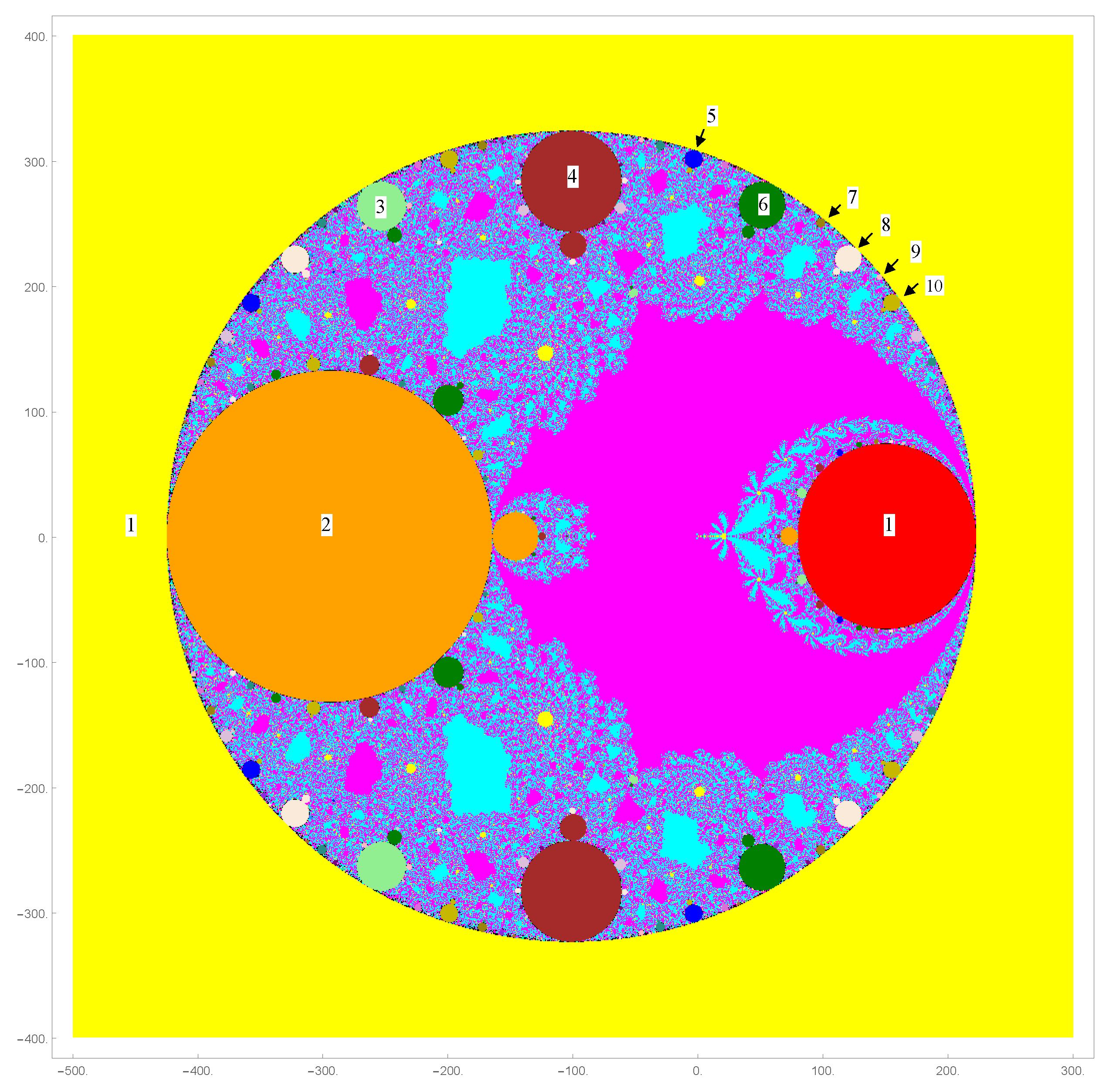
Judging from the parameter spaces in Figure 4, we instantly find a number of typical regions identified by arrow numbers $1\le q\le 10$. With $\lambda$ selected in a region identified by q, the critical orbit approaches to a q-periodic point of J. Note that the possible fixed points of $J(z;\lambda )$ from Equation (13) are $0,1,\infty$ and $\xi \left(\lambda \right)$ given by the roots of $T(z;\lambda )$. Similarly, Equation (12) gives the possible critical points given by the roots of $Q(z;\lambda )$. Since $J(0;\lambda )=0$, $J(-1;\lambda )=1=J(1;\lambda )$, $J(\infty ;\lambda )=\infty$ for any $\lambda \in \mathbb{C}$ and $J\left(\zeta \right(\lambda );\lambda )$ is $\lambda$-dependent, one should pay attention to the orbit behavior of a $\lambda$-dependent critical point $\zeta \left(\lambda \right)$ as $\lambda$ varies in the complex plane. Such an orbit behavior of $\zeta \left(\lambda \right)$ is effectively characterized by tracing the relevant limit behavior such that

$$\underset{n\to \infty }{lim}{J}^n(\zeta \left(\lambda \right);\lambda )=\gamma \in \overline{\mathbb{C}}.$$

If $\gamma$ is not a constant but bounded, then the orbit of $\zeta \left(\lambda \right)$ will approach a non-periodic but bounded orbit. On the other hand, if $\gamma$ is constant, then we write $n=pk+q$ for any $p\in \mathbb{N}$ with $q\in \{0,1,2,\cdots ,p-1\}$. Thus, we obtain

$$\underset{n\to \infty }{lim}{J}^n(\zeta \left(\lambda \right);\lambda )=\underset{k\to \infty }{lim}{J}^{pk+q}(\zeta \left(\lambda \right);\lambda )=J^q\circ (\underset{k\to \infty }{lim}{J}^{pk}(\zeta \left(\lambda \right);\lambda )=J^q(\zeta \left(\gamma \right);\gamma )=\gamma \in \overline{\mathbb{C}},$$

implying that $\gamma$ is a q-periodic point. In case $\gamma =\xi \left(\lambda \right)$, then

$$J^q(\xi \left(\lambda \right);\lambda )=\xi \left(\lambda \right)forq\in \{0,1,2,\cdots ,p-1\},$$

which implies that $\xi \left(\lambda \right)$ is any attracting q-periodic point due to $J^q(\xi \left(\lambda \right);\lambda )$ being a bivariate rational function of z and $\lambda$; note that $q=0$ induces a non-periodic bounded point. Hence, any attracting q-periodic components occur along the boundary $\partial \mathit{Y}$ as seen in $\mathcal{P}$.

We further observe the following bifurcation phenomena as $\lambda$ varies: when $\lambda$ crosses the boundary $\partial \mathit{Y}$, the fixed point $\xi \left(\lambda \right)=1$ loses its stability, but another non-periodic bounded point or attracting q-periodic fixed point will gain their stability and begin to emerge along the boundary $\partial \mathit{Y}$.

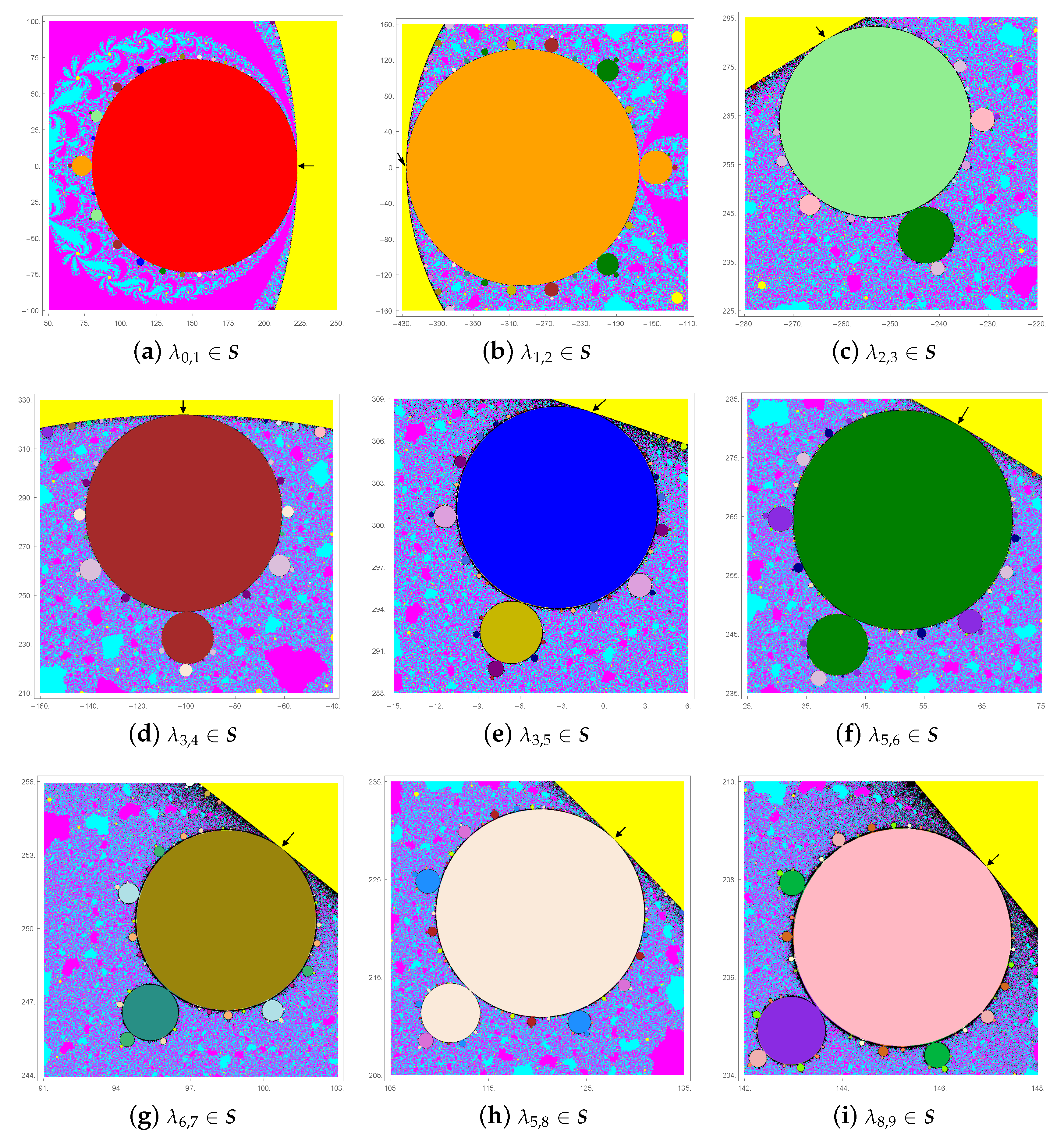
Figure 5 displays components where q-periodic orbits are generated with $q\in \{0,1,2,3,\cdots ,\}$ budding from the component Y associated with the fixed point $\xi \left(\lambda \right)=1$. The q-periodic satellite components with $q\in \mathbb{N}$ can be seen, some of which are indicated by numbers q with arrow lines. Their boundaries are inscribed along the boundary of Y in the manner of Farey sequence [27]. The number of q-periodic satellite components can be determined by means of the lengths of this Farey sequence, which will be discussed later in Section 5.1.2.

5.1. Locating and Counting Bifurcation Points Budding from Y

We first introduce some notions for a qualitative as well as a quantitative bifurcation analysis. A component $\mathit{H}$ in $\mathcal{P}$ is called hyperbolic if $J(z;\lambda )$ has a finite attracting cycle for each given $\lambda \in \mathit{H}$; here, the word ’hyperbolic’ comes from the meaning of ’hyperbolicity’ [28] of a rational function, not from that of a fixed point of a dynamical system. It turns out that $\mathit{H}$ is an open set with infinitely many connected components, each of which is characterized by the period of the corresponding cycle. From now on, we will omit the word ’hyperbolic’ to describe components under consideration as simply as possible. The notions for satellite and primitive components should be referred to those described in [21]. The primitive components are indeed standing alone themselves.

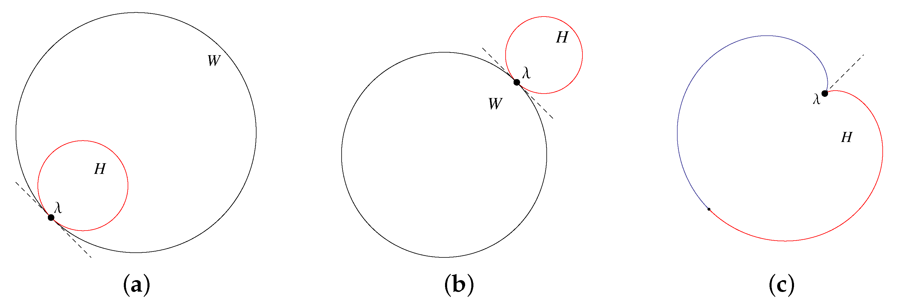
Figure 6 well illustrates typical bifurcation geometries between such two aforementioned components $\mathit{H}$ and $\mathit{W}$. The location of the control parameter where $\mathit{H}$ buds from $\mathit{W}$ is said to be the root point [21] of $\mathit{H}$. If we view this kind of budding phenomenon from the side of $\mathit{W}$, then the root point can be regarded as a bifurcation point of $\mathit{W}$ where it splits into two components based on the lexical meaning of the word bifurcation.

To develop a technique tracking down such bifurcation points in $\mathcal{P}$, it is useful to define a k-periodic (hyperbolic) component ${\mathit{H}}_k=\{\lambda \in \mathbb{C}:J(z;\lambda )\mathrm{that}\mathrm{has}\mathrm{an}\mathrm{attracting}k-\mathrm{cycle}\}$ as a subset of $\mathit{H}$. For notational convenience, we now write $J(z;\lambda )$ as $J_{\lambda }\left(z\right)$ to locate bifurcation points under discussion. We further characterize ${\mathit{H}}_k$ by the following expression:

$${\mathit{H}}_k=\{\lambda \in \mathbb{C}:\mathrm{there}\mathrm{exis}\xi \mathrm{such}\mathrm{that}{J}_{\lambda }^k\left(\xi \right)=\xi \mathrm{and}|\frac{d}{dz}{J}_{\lambda }^k\left(z\right){|}_{z=\xi }<1\}.$$

(15)

In particular, ${\mathit{H}}_1$ plays the role of a main component from which finite-periodic components are born. A choice of $\lambda$-dependent free critical points $\zeta \left(\lambda \right)$ satisfying $Q(\zeta ;\lambda )=0$ in Equation (12) would produce $\mathcal{P}$ whose $\lambda$-value leads us to a long-term dynamical behavior with possible periodic, non-periodic or chaotic orbits, as $\lambda$ varies in the complex plane. An analysis of periodic orbits of $\zeta \left(\lambda \right)$ in the long run is of our current interest. To fully characterize ${\mathit{H}}_1$, we need to inspect the strange fixed point $\xi \left(\lambda \right)=1$ with $\xi \left(\lambda \right)$ given by a root of $T(\xi ;\lambda )$ in Equation (13). In the current analysis, we are limited to considering satellite components ${\mathit{H}}_q$ born along the stability circle S being associated with the strange fixed point $\xi \left(\lambda \right)=1$.

5.1.1. Tracking down Bifurcation Points of Satellite Components Budding from Y

As we can see parameter spaces $\mathcal{P}$ in Figure 4, various components of finite periods bud from the boundary S of Y. It would be better to call Y the main component due to the fact that satellite components of finite periods bud from Y as typically configured with $\mathit{W}=\mathit{Y}$ in Figure 6a.

Let $\partial \mathit{Y}$ denote the boundary of Y and $\lambda$ be a boundary point of $\partial \mathit{Y}$. If a period-q component ${\mathit{H}}_q$ emerges at $\lambda$, then it is natural to name such $\lambda$ as the period-q bifurcation point. If a primitive component ${\mathit{H}}_q$ emerges at $\lambda$, then such a bifurcation point $\lambda$ usually turns out to be a cusp point at which two branches of a boundary curve $\partial {\mathit{H}}_q$ meet together such that the tangent of each branch is equal.

Suppose that a period-q component ${\mathit{H}}_q$, as shown in Figure 6, buds at $\lambda \in \partial \mathit{Y}\bigcap \partial {\mathit{H}}_q$ from Y for a given $q\in \mathbb{N}$. Then, the q-periodic point $\xi$ of J satisfies the following relations:

$$\left\{\begin{array}{c}{J}_{\lambda }^q\left(\xi \right)=J_{\lambda }\left(\xi \right)=\xi ,\hfill \\ \frac{d}{dz}{J}_{\lambda }^q{\left(z\right)|}_{z=\xi }={\beta }^q,\hfill \end{array}\right.$$

(16)

where $J_{\lambda }\left(\xi \right)\equiv J(\xi ;\lambda )$ and $\beta =J_{\lambda }^{\prime }\left(\xi \right)$. Let $\xi =\left|\xi \right|e^{it}$ be a parametric representation for $t\in [0,2\pi ]$. It will be shown that relation ${\beta }^q=1$ is satisfied at $\lambda$ where Y and ${\mathit{H}}_q$ share the common tangent line as illustrated in Figure 6.

Due to the fact that $J_{\lambda }\left(\xi \left(t\right)\right)$ in Equation (11) is a bivariate rational function of both variables $\xi$ and $\lambda$, we solve $J_{\lambda }\left(\xi \left(t\right)\right)=\xi \left(t\right)$ for $\lambda$ to obtain:

$$\lambda \left(t\right)=\Phi \left(\xi \left(t\right)\right)=\Phi \left(J_{\lambda }^q\left(\xi \left(t\right)\right)\right),$$

(17)

with $\Phi \left(z\right)$ as a rational function. Thus, such $\lambda \left(t\right)$ will trace a parametric curve in $\mathbb{C}$ as a function of t. As a result, the derivative $\frac{d\lambda }{dt}$ computed at the fixed point $\xi$ is given by:

$$\begin{array}{c}\hfill \frac{d\lambda }{dt}=\frac{d\Phi \left(z\right(t\left)\right)}{dz}·\frac{dz}{dt}{|}_{z=\xi }=\frac{d\Phi (J_{\lambda }^q\left(z\left(t\right)\right)}{dz}·\frac{dz}{dt}{|}_{z=\xi }=\frac{d\Phi \left(z\right(t\left)\right)}{dz}·{\beta }^q·\frac{dz}{dt}{|}_{z=\xi },\end{array}$$

(18)

which implies that ${\beta }^q=1$ by directly comparing the second and last relations in Label (18).

Note that $\frac{d\lambda }{dt}$ represents the common tangent line evaluated at the period-q point $\xi \left(t\right)$ in the direction of t. Solving process of ${\beta }^q=1$ suggests us the following notion of $\ell /q$–bifurcation point as introduced in the work of [16]:

Definition 2.

For a given $q\in \mathbb{N}$, let $\beta \left(\lambda \right)=e^{i2\pi \ell /q}$, with $\ell \in \left\{0,1,2,\cdots ,q-1\right\}$ and gcd$(\ell ,q)=1$ for $\ell \ne 0$, then λ is called the $\ell /q$–bifurcation point of Y or $\ell /q$–root point of ${\mathit{H}}_q$.

According to the values of $\beta$ in Definition 2, the fold bifurcation and the flip bifurcation respectively occur with $(\ell ,q)=(0,1)$ and $(\ell ,q)=(1,2)$, while the Neimark–Sacker bifurcation occurs with all other values of $(\ell ,q)$.

In view of Theorem 2 and by a close inspection of the parameter space $\mathcal{P}$, we desire to locate the $\ell /q$–bifurcation point $\lambda$ along $\partial \mathit{Y}$. To this end, from relation

$$\beta =J_{\lambda }^{\prime }{\left(\xi \right)|}_{\xi =1}=\frac{1296}{405+4\lambda },$$

we find $\lambda$ in terms of $\beta$:

$$\lambda =-\frac{405}{4}+\frac{324}{\beta }.$$

(19)

After substituting $\beta =e^{2i\pi \ell /q}$ in Definition 2, we obtain the following proposition.

Proposition 3.

The desired $\ell /q$–bifurcation points ${\lambda }_{\ell ,q}$ along $\partial \mathit{Y}$ are found to be

$${\lambda }_{\ell ,q}=-\frac{405}{4}+\frac{324}{e^{i2\pi \ell /q}},$$

for a given $q\in \mathbb{N}$ with $\ell \in \left\{0,1,2,\cdots ,q-1\right\}$ and gcd$(\ell ,q)=1$ for $\ell \ne 0$.

Table 2. Selected  $\ell /q$–bifurcation points ${\lambda }_{\ell ,q}$ for $1\le q\le 10$.

q	ℓ
	0	1	2	3	4	5	6	7	8	9
1	222.75
2		−425.25
3		$\left(\begin{array}{c}-263.25\\ -280.592\end{array}\right)*$	$\left(\begin{array}{c}-263.25\\ 280.592\end{array}\right)$
4		$\left(\begin{array}{c}-101.25\\ -324\end{array}\right)$		$\left(\begin{array}{c}-101.25\\ 324\end{array}\right)$
5		$\left(\begin{array}{c}-1.12849\\ -308.142\end{array}\right)$	$\left(\begin{array}{c}-363.372\\ -190.442\end{array}\right)$	$\left(\begin{array}{c}-363.372\\ 190.442\end{array}\right)$	$\left(\begin{array}{c}-1.12849\\ 308.142\end{array}\right)$
6		$\left(\begin{array}{c}60.75\\ -280.592\end{array}\right)$				$\left(\begin{array}{c}60.75\\ 280.592\end{array}\right)$
7		$\left(\begin{array}{c}100.761\\ -253.313\end{array}\right)$	$\left(\begin{array}{c}-173.347\\ -315.877\end{array}\right)$	$\left(\begin{array}{c}-393.164\\ -140.578\end{array}\right)$	$\left(\begin{array}{c}-393.164\\ 140.578\end{array}\right)$	$\left(\begin{array}{c}-173.347\\ 315.877\end{array}\right)$	$\left(\begin{array}{c}100.761\\ 253.313\end{array}\right)$
8		$\left(\begin{array}{c}127.853\\ -229.103\end{array}\right)$		$\left(\begin{array}{c}-330.353\\ -229.103\end{array}\right)$		$\left(\begin{array}{c}-330.353\\ 229.103\end{array}\right)$		$\left(\begin{array}{c}127.853\\ 229.103\end{array}\right)$
9		$\left(\begin{array}{c}146.948\\ -208.263\end{array}\right)$	$\left(\begin{array}{c}-44.988\\ -319.078\end{array}\right)$		$\left(\begin{array}{c}-405.71\\ -110.815\end{array}\right)$	$\left(\begin{array}{c}-405.71\\ 110.815\end{array}\right)$		$\left(\begin{array}{c}-44.988\\ 319.078\end{array}\right)$	$\left(\begin{array}{c}146.948\\ 208.263\end{array}\right)$
10		$\left(\begin{array}{c}160.872\\ -190.442\end{array}\right)$		$\left(\begin{array}{c}-201.372\\ -308.142\end{array}\right)$				$\left(\begin{array}{c}-201.372\\ 308.142\end{array}\right)$		$\left(\begin{array}{c}160.872\\ 190.442\end{array}\right)$

*: $\left(\begin{array}{c}-263.25\\ -280.592\end{array}\right)$ ≡ −263.25 − 280.592i, i = $\sqrt{-1}$.

lists some values of ${\lambda }_{\ell ,q}$ for $1\le q\le 10$, and some of them are indicated by arrow lines in Figure 5. The $0/1$-bifurcation point is of fold bifurcation and the $1/2$-bifurcation point is of flip bifurcation. All other $\ell /q$–bifurcation points are of Neimark–Sacker bifurcation. It is interesting to observe intuitively that q-periodic components ${\mathit{H}}_q$ for $(q=2,4,6,\cdots ,)$ are born in descending order of its area size monotonically clockwise along the upper half-circle of S.

5.1.2. Counting Bifurcation Points of Satellite Components Budding from Y

The Farey sequence ${\mathcal{F}}_n$ is a set of rational numbers $\frac{p}{q}$ with coprime integers p and q satisfying $0\le p\le q\le n$ arranged in ascending order by size. Charles Haros [29] discovered this sequence in 1806, but Augustin-Louis Cauchy [30] named it after geologist John Farey [31].

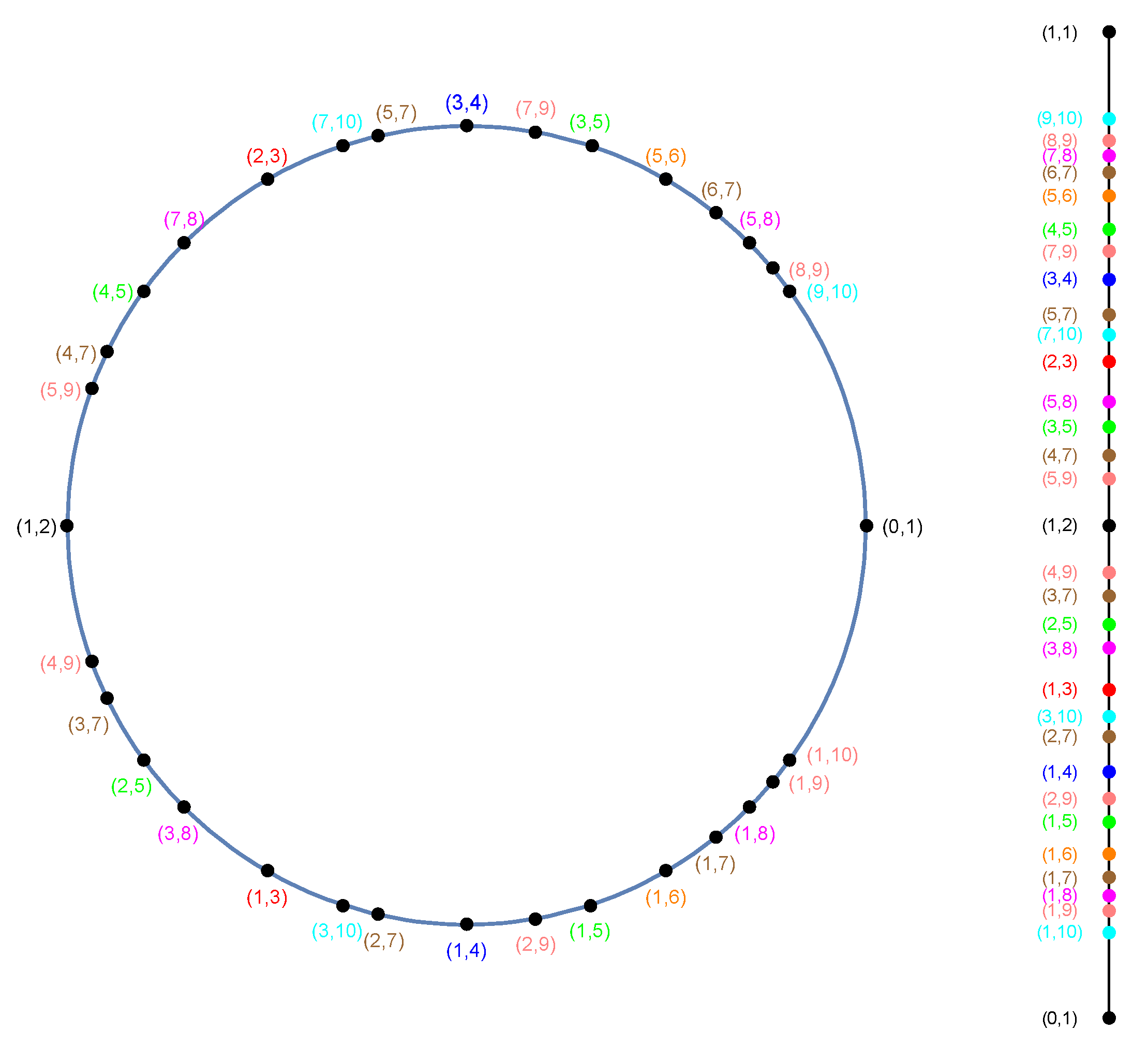
On the left side of Figure 7, we find dots with ordered pairs of numbers $(\ell ,q)$ indicating circumferential locations of bifurcation points ${\lambda }_{\ell ,q}$ along the boundary of Y. Furthermore, on the right side of Figure 7, we also find their homeomorphic images onto the upright unit interval.

Thus, $\frac{\ell }{q}\in {\mathcal{F}}_n$ if $0\le \ell \le q\le n$ with coprime integers ℓ and q, treating the numbers $0\equiv \frac{0}{1}$ and $1\equiv \frac{1}{1}$. For example,

$${\displaystyle {\mathcal{F}}_1=\left\{\frac{0}{1},\frac{1}{1}\right\},{\mathcal{F}}_2=\left\{\frac{0}{1},\frac{1}{2},\frac{1}{1}\right\},{\mathcal{F}}_3=\left\{\frac{0}{1},\frac{1}{3},\frac{1}{2},\frac{2}{3},\frac{1}{1}\right\},\cdots .}$$

Here, $\frac{1}{1}$ simply indicates the top end of the upright unit interval and matches the circumferential location with $\frac{0}{1}$. As described in [27], we introduce the well-known Farey addition: if $\frac{a}{b}$ and $\frac{c}{d}$ with $\frac{a}{b}<\frac{c}{d}$ are Farey neighbors, then the mediant is given by: ${\displaystyle \frac{a}{b}⨁\frac{c}{d}=\frac{a+c}{b+d}}$ and satisfies ${\displaystyle \frac{a}{b}<\frac{a+c}{b+d}<\frac{c}{d}}$. Figure 7 illustrates such properties as typically shown by an example: ${\displaystyle \frac{1}{3}<\frac{3}{8}<\frac{2}{5}}$.

Indeed, the total number of bifurcation points of ${\lambda }_{\ell ,q}$ with $q\le n$ is given by $|{\mathcal{F}}_n|-1$, with $|{\mathcal{F}}_n|$ as the length of ${\mathcal{F}}_n$ stated in the theorem below.

Theorem 4.

With $\varphi \left(k\right)$ as Euler’s totient function, the length of Farey sequence ${\mathcal{F}}_n$ is given by:

$$|{\mathcal{F}}_n|=1+\sum _{k=1}^n\varphi \left(k\right).$$

Proof. 

The Farey Sequence ${\mathcal{F}}_{n-1}$ contains every reduced fraction with denominators at most $n-1$. If we want to create $F_n$ we have to add all reduced fractions with a denominator that is coprime to n. Therefore, $|{\mathcal{F}}_n|=|{\mathcal{F}}_{n-1}|+\varphi \left(n\right)$ with $|{\mathcal{F}}_1|=2=1+\varphi \left(1\right)$. Hence, the proof is completed. □

A result of the above theorem directly leads us to:

Corollary 3.

The total number of q-periodic satellite components budding from Y with $q\le n$ is given by the summatory Euler’s totient function:

$$\Phi \left(n\right)=\sum _{k=1}^n\varphi \left(k\right).$$

6. Discussion with Concluding Remarks

Under the Möbius conjugacy map $M\left(z\right)=\frac{z-a}{z-b},(a\ne b$) applied to a simple quadratic polynomial, we have explored bifurcation phenomena behind the long-term orbit of a free critical point under the action of Jarratt-like iterative map (2) with $H\left(t\right)$ in Equation (3). The bifurcation behavior for occurrence of q-periodic satellite components has been analyzed in the parameter spaces in view of elementary theory of plane geometry. The boundary of the main component where the $\lambda$-dependent critical orbit of $J_{\lambda }\left(z\right)$ tends to the fixed point 1 has been found to be a circle along which infinitely many periodic satellite components are born. The linear stability theory and the elementary viewpoint of plane geometry on the existence of the common tangent line between the boundary of the main and budding components have enabled us to successfully locate bifurcation points where new satellite components arise. In addition, a theory of the Farey sequence plays an essential role in counting the number of such bifurcation points characterized by inscription-type bifurcation geometries illustrated in Figure 6a.

Future study should focus not only on long-term orbit behavior in the parameter spaces for bifurcation phenomena related to satellite and primitive components, but also convergence behavior dependent on initial values in the dynamical planes.