Valuing Guaranteed Minimum Death Benefits by Cosine Series Expansion

Abstract

Recently, the valuation of variable annuity products has become a hot topic in actuarial science. In this paper, we use the Fourier cosine series expansion (COS) method to value the guaranteed minimum death benefit (GMDB) products. We first express the value of GMDB by the discounted density function approach, then we use the COS method to approximate the valuation Equations. When the distribution of the time-until-death random variable is approximated by a combination of exponential distributions and the price of the fund is modeled by an exponential Lévy process, explicit equations for the cosine coefficients are given. Some numerical experiments are also made to illustrate the efficiency of our method.

1. Introduction

The guaranteed minimum death benefit (GMDB) is a common rider embedded in variable annuity products that promises a minimum payout upon the death of the insured. In this product, policyholders first pay premiums to the insurance company, and then, investment accounts are established for capital investment. When the insured dies, a payment shall be given to the designated beneficiary, and the payout amount depends on the performance of the policyholder’s account. This mechanism not only provides insurance guarantee for policyholders, but also has the opportunity to benefit from the financial market, which appeals to customers.

For $t\ge 0$, let $S\left(t\right)=S\left(0\right)e^{X\left(t\right)}$ denote the price of a stock fund or mutual fund at time t. For a person currently aged x, let $T_x$ denote the remaining lifetime, called the time-until-death random variable hereafter. Moreover, we assume $T_x$ is independent with the asset price process $S\left(t\right)$ throughout this paper. Consider a GMDB rider that guarantees a payment of $b\left(S\left(T_x\right)\right)$ to the beneficiary when the insured dies, where $b(·)$ is an equity-linked death benefit function. For a constant force of interest $\delta \ge 0$, we are interested in valuing the following expectation:

$$\begin{array}{c}\hfill V_x:=E\left[e^{-\delta T_x}b\left(S\left(T_x\right)\right)\right],\end{array}$$

(1)

which represents a fair price for an equity-linked life-contingent payment at $T_x$. Since most contracts have a finite expiry date, we can modify (1) by introducing an expiry date T and consider:

$$\begin{array}{c}\hfill V_{x,T}:=E\left[e^{-\delta T_x}b\left(S\left(T_x\right)\right)\mathbf{I}(T_x\le T)\right],\end{array}$$

(2)

where $\mathbf{I}\left(A\right)$ denotes the indicator function of event A.

We are also interested in the case when the death benefit amount depends on two stocks (or stock funds). Let ${\{S_1\left(t\right),S_2\left(t\right)\}}_{t\ge 0}$ denote the price process of two stocks, and let:

$$X_i\left(t\right)=ln(S_i\left(t\right)/S_i\left(0\right)),i=1,2,t\ge 0.$$

In the sequel, it is also assumed that $T_x$ is independent with both $S_1\left(t\right)$ and $S_2\left(t\right)$. Accordingly, we are interested in evaluating the following expectations:

$${\overline{V}}_x:=E\left[e^{-\delta T_x}b(S_1\left(T_x\right),S_2\left(T_x\right))\right],{\overline{V}}_{x,T}:=E\left[e^{-\delta T_x}b(S_1\left(T_x\right),S_2\left(T_x\right))\mathbf{I}(T_x\le T)\right].$$

Recently, the valuation of the GMDB product has drawn many researchers’ attention. Under an exponential mortality law, Milevsky and Posner [1] proposed a risk-neutral framework to derive valuation equations for GMDB contracts. Besides, they conducted a numerical study under the Gompertz-Makeham law. Later, in Bauer et al. [2], they supposed that the death should only occur at the policy anniversary date, which facilitates a discrete numerical valuation approach for fairly valuing varieties of guaranteed riders, including GMDB. Gerber et al. [3] proposed a discounted density approach to value GMDB in a Brownian motion risk model, and their results were extended by Gerber et al. [4] and Siu et al. [5] to the jump diffusion model and the regime-switching jump diffusion model, respectively. Based on the fact that the combination of exponential distributions is weakly dense on the set of probability functions defined on $[0,\infty )$ (see Dufresne [6] and Ko and Ng [7]), we notice that the density function of the time-until-death random variable was approximated by a linear combination of exponential distributions in Gerber et al. [3,4] and Siu et al. [5]. More recently, Zhang and Yong [8] and Zhang et al. [9] used two different methods to value GMDB products. Recent related literature can be found in Dai et al. [10], Bélanger et al. [11], Kang and Ziveyi [12], Asmussen et al. [13], and Zhou and Wu [14].

When the density function of the time-until-death random variable is approximated by a linear sum of exponential distributions, Gerber et al. [3,4,15] derived explicit valuation equations for GMDB contracts under various payoffs. The simplicity of using a combination of exponential distributions is excellent, but they are not representative of reality. A direct way to calibrate this is to use life table data. In Ulm [16,17], he emphasized the valuation of GMDB products under mortality laws, such as the De Moivre law of mortality and the Makeham law of mortality. A similar consideration could be found in Liang et al. [18]. They novelly introduced the piecewise constant forces of the mortality assumption to describe the time-until-death variable, then decomposed the valuation problem and presented explicit valuation equations for GMDB.

Except the aforementioned assumptions on the time-until-death random variable, the modeling of the asset process has attracted the attention of scholars. Brownian motion was widely used to model the log-asset price process, which was adopted in Milevsky and Posner [1], Bauer et al. [2] (Section 4), Gerber et al. [3], and Liang et al. [18]. In the field of financial markets, this case is basically a Black-Scholes framework. However, more processes could be also implemented. In Gerber et al. [4], Kou’s jump model was used as the log-asset process. A counterpart study of Gerber et al. [3] was referred to by Gerber et al. [15], in which a random walk exponentially generates the price process. To study the valuation issue in a different perspective, scholars turned to the regime-switching model, which was used to investigate the performance of an object subject to the economic changes in financial markets. In the literature, interest readers can refer to Fan et al. [19], Siu et al. [5], Ignatieva et al. [20], and Hieber [21].

In Fang and Oosterlee [22], a highly-efficient option pricing method was proposed to price European options. The method was based on the Fourier cosine series expansions, and it is now called the cosine series expansion (COS) method in the literature. The COS method is quite easy to implement to approximate an integrable function as long as the objective function has a closed-form Fourier transform. The one-dimensional COS (1D COS) method in [22] was extended to the two-dimensional COS method (2D COS) by Ruijter and Oosterlee [23] to price financial options in two-dimensional asset price processes. Leitao et al. [24] proposed a data-driven COS method. Except for option pricing, this method has been adopted in insurance ruin theory. For example, Chau et al. [25,26] used the 1D COS method to compute the ruin probability and the expected discounted penalty function; Zhang [27] approximated the density function of the time to ruin by both 1D and 2D COS methods; Yang et al. [28] proposed a nonparametric estimator for the deficit at ruin by the 2D COS method; Wang et al. [29] and Huang et al. [30] used the 1D COS method to estimate the expected discounted penalty function under some risk models with stochastic premium income. The COS method has also been used by some authors to value variable annuities. For example, Deng et al. [31] used the 1D COS method for equity-indexed annuity products under general exponential Lévy models; Alonso-García et al. [32] extended the 1D COS method to the pricing and hedging of variable annuities embedded with guaranteed minimum withdraw benefit riders. The latest research on Fourier transform was given by Zhang et al. [33], Chan [34], Zhang and Liu [35], Have and Oosterlee [36], Shimizu and Zhang [37], Tour [38], Zhang [39], and Wang et al. [40].

The discounted density method proposed by Gerber et al. [3,4] can be successfully used to value GMDB products when the log-return process is the Brownian motion or Kou’s jump diffusion model. Under these two models, the density functions have some closed-form expressions. However, in practice, we cannot obtain the closed-from expression for the discounted density function. In this paper, we use the COS method to approximate the discounted density function, which is applicable since most of the widely-used Lévy processes have explicit characteristic functions. To the best of our knowledge, this is the first paper exploring the COS method on numerical valuation of the GMDB product under the general exponential Lévy models. In particular, there are few papers on GMDB valuation dependent on two stock prices in the literature, and this is the first paper dealing with this problem.

This paper aims to value the GMDB contracts in a risk-neutral framework, mainly by numerically solving Equations (1) and (2). In subsequent sections, we first briefly recall the COS method in Fang and Oosterlee [22], then adopt the method to approximate $V_x$ and $V_{x,T}$ in the one-dimensional framework. We define auxiliary functions to simplify deductions and display equations under different payoffs in Section 2. Motivated by Gerber et al. [3], we consider the situation where the density function of $T_x$ is approximated by a linear combination of exponential distributions, and calculate cosine coefficients in Section 4.1. Under the multi-dimensional case, we shed light on a two-dimensional framework in Section 3. Finally, numerical examples are presented in Section 4, in which we display tables and figures to illustrate the performance of our proposed approach.

2. 1D COS Approximation

In the section, we shall use the 1D COS method to compute $V_x$ and $V_{x,T}$. The idea of the 1D COS method is that every absolutely integrable function f can be approximated on a truncated domain $[a_1,a_2]$ by a truncated Fourier cosine series with N terms,

$$f\left(y\right)\approx \sum _{k=0}^{N-1}{}^{\prime }{\mathcal{A}}_k(f,a_1,a_2)cos\left(k\pi \frac{y-a_1}{a_2-a_1}\right),$$

(3)

where $\sum {}^{\prime }$ means that the first term in the summation has half weight, and the cosine coefficients are given by:

$${\mathcal{A}}_k(f,a_1,a_2)=\frac{2}{a_2-a_1}\mathrm{Re}\left\{\mathcal{F}f\left(\frac{k\pi }{a_2-a_1}\right)exp\left(-i\frac{k{a}_1\pi }{a_2-a_1}\right)\right\}.$$

(4)

Here, $\mathcal{F}f\left(s\right)=\int e^{isy}f\left(y\right)dy$, $s\in \mathbb{R}$, is the Fourier transform of f, and $\mathrm{Re}(·)$ means taking the real part.

Let $f_{T_x}(·)$ denote the probability density function of $T_x$, and for $t>0$, let $f_{X\left(t\right)}(·)$ be the probability density function of $X\left(t\right)$. By changing the order of integrals, we can obtain:

$$\begin{array}{ccc}\hfill V_x& =& {\int }_0^{\infty }E\left[e^{-\delta t}b\left(S\left(t\right)\right)\right]f_{T_x}\left(t\right)dt\hfill \\ \hfill & =& {\int }_0^{\infty }{e}^{-\delta t}{\int }_{-\infty }^{\infty }b\left(S\left(0\right)e^y\right)f_{X\left(t\right)}\left(y\right)dy{f}_{T_x}\left(t\right)dt\hfill \\ \hfill & =& {\int }_{-\infty }^{\infty }b\left(S\left(0\right)e^y\right)f_{X\left(T_x\right)}^{\delta }\left(y\right)dy,\hfill \end{array}$$

(5)

where:

$$f_{X\left(T_x\right)}^{\delta }\left(y\right)={\int }_0^{\infty }{e}^{-\delta t}{f}_{X\left(t\right)}\left(y\right)f_{T_x}\left(t\right)dt$$

(6)

is the discounted density function of the random variable $X\left(T_x\right)$. Similarly, for the T-year life-contingent option, we have:

$$\begin{array}{c}\hfill V_{x,T}={\int }_{-\infty }^{\infty }b\left(S\left(0\right)e^y\right)f_{X\left(T_x\right),T}^{\delta }\left(y\right)dy,\end{array}$$

(7)

where:

$$f_{X\left(T_x\right),T}^{\delta }\left(y\right)={\int }_0^T{e}^{-\delta t}{f}_{X\left(t\right)}\left(y\right)f_{T_x}\left(t\right)dt.$$

(8)

We shall implement the 1D COS method to compute the integrals in (5) and (7). Instead of expanding the discounted densities $f_{X\left(T_x\right)}^{\delta }$ and $f_{X\left(T_x\right),T}^{\delta }$ via Fourier cosine series, we shall consider the following auxiliary functions:

$$g_n^{\delta }\left(y\right)=e^{ny}{f}_{X\left(T_x\right)}^{\delta }\left(y\right),g_{n,T}^{\delta }\left(y\right)=e^{ny}{f}_{X\left(T_x\right),T}^{\delta }\left(y\right),n\ge 0.$$

Suppose that both $g_n^{\delta }$ and $g_{n,T}^{\delta }$ belong to $L^1\left(\mathbb{R}\right)$, then by Equations (3) and (4), we have:

$$g_n^{\delta }\left(y\right)\approx \sum _{k=0}^{N-1}{}^{\prime }{\mathcal{A}}_k(g_n^{\delta },a_1,a_2)cos\left(k\pi \frac{y-a_1}{a_2-a_1}\right)$$

(9)

and:

$$g_{n,T}^{\delta }\left(y\right)\approx \sum _{k=0}^{N-1}{}^{\prime }{\mathcal{A}}_k(g_{n,T}^{\delta },a_1,a_2)cos\left(k\pi \frac{y-a_1}{a_2-a_1}\right).$$

(10)

Remark 1.

The cosine coefficients ${\mathcal{A}}_k(g_n^{\delta },a_1,a_2)$ and ${\mathcal{A}}_k(g_{n,T}^{\delta },a_1,a_2)$ can be explicitly computed when ${\left\{X\left(t\right)\right\}}_{t\ge 0}$ is a Lévy process and $f_{T_x}$ is a combination of exponential density function. To this end, it suffices to specify the Fourier transforms $\mathcal{F}{g}_n^{\delta }$ and $\mathcal{F}{g}_{n,T}^{\delta }$. Suppose that ${\left\{X\left(t\right)\right\}}_{t\ge 0}$ (with $X\left(0\right)=0$) is a Lévy process with characteristic function:

$${\varphi }_{X\left(t\right)}\left(s\right)=E[e^{isX\left(t\right)}]=e^{t{\mathrm{\Psi }}_X\left(s\right)},s\in \mathbb{R},$$

(11)

where ${\mathrm{\Psi }}_X\left(s\right)=ln(E[e^{isX\left(1\right)}])$ is called the characteristic exponent. Furthermore, suppose that:

$$f_{T_x}\left(t\right)=\sum _{j=1}^m{A}_j{\alpha }_j{e}^{-{\alpha }_{j}t},t>0,$$

(12)

where ${\alpha }_j>0$ and ${\sum }_{j=1}^m{A}_j=1$. Under these assumptions, one easily obtains:

$$\mathcal{F}{g}_n^{\delta }\left(s\right)=\sum _{j=1}^m\frac{A_j{\alpha }_j}{\delta +{\alpha }_j-{\mathrm{\Psi }}_X(s-in)}$$

(13)

and:

$$\mathcal{F}{g}_{n,T}^{\delta }\left(s\right)=\sum _{j=1}^m{A}_j{\alpha }_j\frac{1-e^{-(\delta +{\alpha }_j-{\mathrm{\Psi }}_X(s-in))T}}{\delta +{\alpha }_j-{\mathrm{\Psi }}_X(s-in)}.$$

(14)

In the sequel, we shall consider three payoff functions.

Case 1. $b\left(s\right)=s$.

In this case, Equations (5) and (7) become:

$$V_x=S\left(0\right){\int }_{-\infty }^{\infty }{g}_1^{\delta }\left(y\right)dy,V_{x,T}=S\left(0\right){\int }_{-\infty }^{\infty }{g}_{1,T}^{\delta }\left(y\right)dy.$$

For small number $c_1$ and large number $c_2$, using Equation (9), we can approximate $V_x$ as follows,

$$\begin{array}{ccc}\hfill V_x& \approx & S\left(0\right){\int }_{c_1}^{c_2}{g}_1^{\delta }\left(y\right)dy\hfill \\ \hfill & \approx & S\left(0\right){\int }_{c_1}^{c_2}\sum _{k=0}^{N-1}{}^{\prime }{\mathcal{A}}_k(g_1^{\delta },a_1,a_2)cos\left(k\pi \frac{y-a_1}{a_2-a_1}\right)dy\hfill \\ \hfill & =& S\left(0\right)\sum _{k=0}^{N-1}{}^{\prime }{\mathcal{A}}_k(g_1^{\delta },a_1,a_2)·{\chi }_k(a_1,a_2,c_1,c_2),\hfill \end{array}$$

(15)

where:

$${\chi }_k(a_1,a_2,c_1,c_2)=\left\{\begin{array}{cc}{\displaystyle \frac{a_2-a_1}{k\pi }\left[sin\left(k\pi \frac{c_2-a_1}{a_2-a_1}\right)-sin\left(k\pi \frac{c_1-a_1}{a_2-a_1}\right)\right],}\hfill & k\ne 0,\hfill \\ c_2-c_1,\hfill & k=0.\hfill \end{array}\right.$$

Similarly, $V_{x,T}$ can be approximated as follows,

$$\begin{array}{c}\hfill V_{x,T}\approx S\left(0\right)\sum _{k=0}^{N-1}{}^{\prime }{\mathcal{A}}_k(g_{1,T}^{\delta },a_1,a_2)·{\chi }_k(a_1,a_2,c_1,c_2).\end{array}$$

(16)

Case 2. $b\left(s\right)=s^n{\mathbf{I}}_{(s>K)}$ with $n\ge 0$ and $K>0$.

Here, the positive constant K denotes the strike price. Put $\kappa =ln(K/S(0\left)\right)$. It follows from Equation (5) that:

$$V_x={\int }_{\kappa }^{\infty }{\left[S\left(0\right)\right]}^n{e}^{ny}{f}_{X\left(T_x\right)}^{\delta }\left(y\right)dy={\int }_{\kappa }^{\infty }{\left[S\left(0\right)\right]}^n{g}_n^{\delta }\left(y\right)dy.$$

Then, using the 1D COS method, we obtain for large number $c_2$,

$$V_x\approx {\left[S\left(0\right)\right]}^n\sum _{k=0}^{N-1}{}^{\prime }{\mathcal{A}}_k(g_n^{\delta },a_1,a_2)·{\chi }_k(a_1,a_2,\kappa ,c_2).$$

(17)

Similarly, for $V_{x,T}$, we have:

$$V_{x,T}\approx {\left[S\left(0\right)\right]}^n\sum _{k=0}^{N-1}{}^{\prime }{\mathcal{A}}_k(g_{n,T}^{\delta },a_1,a_2)·{\chi }_k(a_1,a_2,\kappa ,c_2).$$

(18)

Remark 2.

For the call option, the payoff is given by:

$$b\left(s\right)={(s-K)}_{+}=s{\mathbf{I}}_{(s>K)}-K{\mathbf{I}}_{(s>K)}.$$

By applying Equations (5) and (17), we obtain:

$$\begin{array}{ccc}\hfill V_x& =& {\int }_{\kappa }^{\infty }S\left(0\right)e^y{f}_{X\left(T_x\right)}^{\delta }\left(y\right)dy-{\int }_{\kappa }^{\infty }K{f}_{X\left(T_x\right)}^{\delta }\left(y\right)dy\hfill \\ \hfill & =& S\left(0\right){\int }_{\kappa }^{\infty }{g}_1^{\delta }\left(y\right)dy-K{\int }_{\kappa }^{\infty }{g}_0^{\delta }\left(y\right)dy\hfill \\ \hfill & \approx & S\left(0\right)\sum _{k=0}^{N-1}{}^{\prime }{\mathcal{A}}_k(g_1^{\delta },a_1,a_2)·{\chi }_k(a_1,a_2,\kappa ,c_2)-K\sum _{k=0}^{N-1}{}^{\prime }{\mathcal{A}}_k(g_0^{\delta },a_1,a_2)·{\chi }_k(a_1,a_2,\kappa ,c_2).\hfill \end{array}$$

(19)

For the T-year life-contingent option, we have:

$$\begin{array}{c}\hfill V_{x,T}\approx S\left(0\right)\sum _{k=0}^{N-1}{}^{\prime }{\mathcal{A}}_k(g_{1,T}^{\delta },a_1,a_2)·{\chi }_k(a_1,a_2,\kappa ,c_2)-K\sum _{k=0}^{N-1}{}^{\prime }{\mathcal{A}}_k(g_{0,T}^{\delta },a_1,a_2)·{\chi }_k(a_1,a_2,\kappa ,c_2).\end{array}$$

(20)

Case 3. $b\left(s\right)=s^n{\mathbf{I}}_{(s<K)}$ with $n\ge 0$ and $K>0$.

By Equation (5) and the 1D COS method, we have for small number $c_1$,

$$\begin{array}{ccc}\hfill V_x& =& {\int }_{\infty }^{\kappa }{\left[S\left(0\right)\right]}^n{g}_n^{\delta }\left(y\right)dy\approx {\left[S\left(0\right)\right]}^n{\int }_{c_1}^{\kappa }{g}_n^{\delta }\left(y\right)dy\hfill \\ \hfill & \approx & {\left[S\left(0\right)\right]}^n\sum _{k=0}^{N-1}{}^{\prime }{\mathcal{A}}_k(g_n^{\delta },a_1,a_2)·{\chi }_k(a_1,a_2,c_1,\kappa ).\hfill \end{array}$$

(21)

Similarly, for $V_{x,T}$, we have:

$$\begin{array}{c}\hfill V_{x,T}\approx {\left[S\left(0\right)\right]}^n\sum _{k=0}^{N-1}{}^{\prime }{\mathcal{A}}_k(g_{n,T}^{\delta },a_1,a_2)·{\chi }_k(a_1,a_2,c_1,\kappa ).\end{array}$$

(22)

Remark 3.

For the put option, the payoff function is given by:

$$b\left(s\right)={(K-s)}_{+}=K{\mathbf{I}}_{(s<K)}-s{\mathbf{I}}_{(s<K)},$$

which together with Equations (21) and (22) gives:

$$V_x\approx K\sum _{k=0}^{N-1}{}^{\prime }{\mathcal{A}}_k(g_0^{\delta },a_1,a_2)·{\chi }_k(a_1,a_2,c_1,\kappa )-S\left(0\right)\sum _{k=0}^{N-1}{}^{\prime }{\mathcal{A}}_k(g_1^{\delta },a_1,a_2)·{\chi }_k(a_1,a_2,c_1,\kappa )$$

(23)

and:

$$V_{x,T}\approx K\sum _{k=0}^{N-1}{}^{\prime }\mathcal{A}(g_{0,T}^{\delta },a_1,a_2)·{\chi }_k(a_1,a_2,c_1,\kappa )-S\left(0\right)\sum _{k=0}^{N-1}{}^{\prime }\mathcal{A}(g_{1,T}^{\delta },a_1,a_2)·{\chi }_k(a_1,a_2,c_1,\kappa ).$$

(24)

3. 2D COS Approximation

In this section, we use the 2D COS method to compute ${\overline{V}}_x$ and ${\overline{V}}_{x,T}$. For a bivariate integrable function f, we denote its Fourier transform by:

$$\mathcal{F}f(s_1,s_2)=\int \int e^{i{s}_{1}y+i{s}_{2}z}f(y,z)dydz,s_1,s_2\in \mathbb{R}.$$

It follows from Ruijter and Oosterlee [23] that f can be approximated on a truncated domain $[a_1,a_2]\times [b_1,b_2]$ by truncated Fourier cosine series expansions with $N_1\times N_2$ terms,

$$f(y,z)\approx \sum _{k_1=0}^{N_1-1}{}^{\prime }\sum _{k_2=0}^{N_2-1}{}^{\prime }{\mathcal{B}}_{k_1,k_2}\left(f\right)cos\left(k_1\pi \frac{y-a_1}{a_2-a_1}\right)cos\left(k_2\pi \frac{z-b_1}{b_2-b_1}\right),$$

(25)

where the cosine coefficients are given by:

$${\mathcal{B}}_{k_1,k_2}\left(f\right)=\frac{1}{2}\left({\mathcal{B}}_{k_1,k_2}^{+}\left(f\right)+{\mathcal{B}}_{k_1,k_2}^{-}\left(f\right)\right)$$

with:

$${\mathcal{B}}_{k_1,k_2}^{\pm }\left(f\right)=\frac{2}{a_2-a_1}\frac{2}{b_2-b_1}\mathrm{Re}\left\{\mathcal{F}f\left(\frac{k_1\pi }{a_2-a_1},\pm \frac{k_2\pi }{b_2-b_1}\right)exp\left(-i{k}_1\pi \frac{a_1}{a_2-a_1}\mp i{k}_2\pi \frac{b_1}{b_2-b_1}\right)\right\}.$$

(26)

For $t>0$, we denote the joint probability density function of $\left(X_1\left(t\right),X_2\left(t\right)\right)$ by $f_{X_1\left(t\right),X_2\left(t\right)}(y,z)$, and for $\delta \ge 0$, define the following discounted density functions:

$$\begin{array}{ccc}\hfill f_{X_1\left(T_x\right),X_2\left(T_x\right)}^{\delta }(y,z)& =& {\int }_0^{\infty }{e}^{-\delta t}{f}_{X_1\left(t\right),X_2\left(t\right)}(y,z)f_{T_x}\left(t\right)dt,\hfill \\ \hfill f_{X_1\left(T_x\right),X_2\left(T_x\right),T}^{\delta }(y,z)& =& {\int }_0^T{e}^{-\delta t}{f}_{X_1\left(t\right),X_2\left(t\right)}(y,z)f_{T_x}\left(t\right)dt.\hfill \end{array}$$

For ${\overline{V}}_x$, by changing the order of integrals, we have:

$$\begin{array}{cc}\hfill {\overline{V}}_x& ={\int }_0^{\infty }E\left[e^{-\delta t}b(S_1\left(t\right),S_2\left(t\right))\right]f_{T_x}\left(t\right)dt\hfill \\ \hfill & ={\int }_0^{\infty }{e}^{-\delta t}{\int }_{-\infty }^{\infty }{\int }_{-\infty }^{\infty }b(S_1\left(0\right)e^y,S_2\left(0\right)e^z)f_{X_1\left(t\right),X_2\left(t\right)}(y,z)dydz{f}_{T_x}\left(t\right)dt\hfill \\ \hfill & ={\int }_{-\infty }^{\infty }{\int }_{-\infty }^{\infty }b(S_1\left(0\right)e^y,S_2\left(0\right)e^z)f_{X_1\left(T_x\right),X_2\left(T_x\right)}^{\delta }(y,z)dydz.\hfill \end{array}$$

(27)

For ${\overline{V}}_{x,T}$, we have:

$$\begin{array}{c}\hfill {\overline{V}}_{x,T}={\int }_{-\infty }^{\infty }{\int }_{-\infty }^{\infty }b(S_1\left(0\right)e^y,S_2\left(0\right)e^z)f_{X_1\left(T_x\right),X_2\left(T_x\right),T}^{\delta }(y,z)dydz.\end{array}$$

(28)

As in Section 2, we shall pay attention to the following auxiliary functions,

$$g_{m,n}^{\delta }(y,z)=e^{my+nz}{f}_{X_1\left(T_x\right),X_2\left(T_x\right)}^{\delta }(y,z),g_{m,n,T}^{\delta }(y,z)=e^{my+nz}{f}_{X_1\left(T_x\right),X_2\left(T_x\right),T}^{\delta }(y,z).$$

Suppose that both $g_{m,n}^{\delta }$ and $g_{m,n,T}^{\delta }$ are absolutely integrable. Then, by Equation (25), we obtain:

$$g_{m,n}^{\delta }(y,z)\approx \sum _{k_1=0}^{N_1-1}{}^{\prime }\sum _{k_2=0}^{N_2-1}{}^{\prime }{\mathcal{B}}_{k_1,k_2}\left(g_{m,n}^{\delta }\right)cos\left(k_1\pi \frac{y-a_1}{a_2-a_1}\right)cos\left(k_2\pi \frac{z-b_1}{b_2-b_1}\right)$$

(29)

and:

$$g_{m,n,T}^{\delta }(y,z)\approx \sum _{k_1=0}^{N_1-1}{}^{\prime }\sum _{k_2=0}^{N_2-1}{}^{\prime }{\mathcal{B}}_{k_1,k_2}(g_{m,n,T}^{\delta })cos\left(k_1\pi \frac{y-a_1}{a_2-a_1}\right)cos\left(k_2\pi \frac{z-b_1}{b_2-b_1}\right).$$

(30)

To calculate cosine coefficients in Equations (29) and (30), we suppose $\left(X_1\left(t\right),X_2\left(t\right)\right)$ is a two-dimensional Lévy process with $X_1\left(0\right)=X_2\left(0\right)=0$. The characteristic exponent is defined by:

$${\mathrm{\Psi }}_{X_1,X_2}(s_1,s_2)=ln(E[e^{i{s}_1{X}_1\left(1\right)+i{s}_2{X}_2\left(1\right)}]).$$

Furthermore, suppose that $f_{T_x}$ is a combination of the exponential density function given by Equation (12). By Fubini theorem, we have:

$$\begin{array}{cc}\mathcal{F}{g}_{m,n}^{\delta }(s_1,s_2)\hfill & =\int \int e^{i{s}_{1}y+i{s}_{2}z}{e}^{my+nz}{f}_{X_1\left(T_x\right),X_2\left(T_x\right)}^{\delta }(y,z)dydz\hfill \\ \hfill & =\int \int e^{(i{s}_1+m)y+(i{s}_2+n)z}{\int }_0^{\infty }{e}^{-\delta t}{f}_{X_1\left(t\right),X_2\left(t\right)}(y,z)f_{T_x}\left(t\right)dtdydz\hfill \\ \hfill & ={\int }_0^{\infty }{e}^{-(\delta -{\mathrm{\Psi }}_{X_1,X_2}(s_1-mi,s_2-ni))t}{f}_{T_x}\left(t\right)dt\hfill \\ \hfill & =\sum _{j=1}^m\frac{A_j{\alpha }_j}{\delta +{\alpha }_j-{\mathrm{\Psi }}_{X_1,X_2}(s_1-mi,s_2-ni)}\hfill \end{array}$$

(31)

and:

$$\begin{array}{cc}\hfill \mathcal{F}{g}_{m,n,T}^{\delta }(s_1,s_2)& ={\int }_0^T{e}^{-(\delta -{\mathrm{\Psi }}_{X_1,X_2}(s_1-mi,s_2-ni))t}{f}_{T_x}\left(t\right)dt\hfill \\ \hfill & =\sum _{j=1}^m{A}_j{\alpha }_j\frac{1-e^{-(\delta +{\alpha }_j-{\mathrm{\Psi }}_{X_1,X_2}(s_1-mi,s_2-ni))T}}{\delta +{\alpha }_j-{\mathrm{\Psi }}_{X_1,X_2}(s_1-mi,s_2-ni)}.\hfill \end{array}$$

(32)

In the sequel, we study the numerical approximation of the value of life-contingent two-asset options. We shall consider the Margrabe option, maximum/minimum option, and geometric option. First, the contingent Margrabe option, also called the exchange option, is considered. Note that its payoff function is:

$${\left[S_1\left(T_x\right)-S_2\left(T_x\right)\right]}_{+}.$$

Then, we have:

$$\begin{array}{cc}\hfill & E\left[e^{-\delta T_x}{[S_1\left(T_x\right)-S_2\left(T_x\right)]}_{+}\right|S_1\left(0\right)<S_2\left(0\right)]\hfill \\ \hfill & ={\int }_0^{\infty }{\int }_{-\infty }^{\infty }{\int }_{-\infty }^{\infty }{e}^{-\delta t}{[S_1\left(0\right)e^y-S_2\left(0\right)e^z]}_{+}·f_{X_1\left(t\right),X_2\left(t\right)}(y,z)f_{T_x}\left(t\right)dydzdt\hfill \\ \hfill & ={\int }_{-\infty }^{\infty }{\int }_{-\infty }^{\infty }{[S_1\left(0\right)e^y-S_2\left(0\right)e^z]}_{+}·f_{X_1\left(T_x\right),X_2\left(T_x\right)}^{\delta }(y,z)dydz\hfill \\ \hfill & =\int {\int }_{(y,z)\in {\mathcal{D}}_1}(S_1\left(0\right)e^y-S_2\left(0\right)e^z)f_{X_1\left(T_x\right),X_2\left(T_x\right)}^{\delta }(y,z)dydz\hfill \\ \hfill & =S_1\left(0\right)\int {\int }_{(y,z)\in {\mathcal{D}}_1}{e}^y{f}_{X_1\left(T_x\right),X_2\left(T_x\right)}^{\delta }(y,z)dydz-S_2\left(0\right)\int {\int }_{(y,z)\in {\mathcal{D}}_1}{e}^z{f}_{X_1\left(T_x\right),X_2\left(T_x\right)}^{\delta }(y,z)dydz\hfill \\ \hfill & =S_1\left(0\right)\int {\int }_{(y,z)\in {\mathcal{D}}_1}{g}_{1,0}^{\delta }(y,z)dydz-S_2\left(0\right)\int {\int }_{(y,z)\in {\mathcal{D}}_1}{g}_{0,1}^{\delta }(y,z)dydz,\hfill \end{array}$$

(33)

where ${\mathcal{D}}_1$ denotes the region $\{(y,z):y-z>ln\frac{S_2\left(0\right)}{S_1\left(0\right)}\}$. Set ${\mathcal{D}}_1^{\prime }={\mathcal{D}}_1\cap ([a_1,a_2]\times [b_1,b_2])$. Utilizing Equation (29), we obtain the following approximation formula:

$$\begin{array}{cc}\hfill & E\left[e^{-\delta T_x}{[S_1\left(T_x\right)-S_2\left(T_x\right)]}_{+}\right|S_1\left(0\right)<S_2\left(0\right)]\hfill \\ \hfill & \approx S_1\left(0\right)\sum _{k_1=0}^{N_1-1}{}^{\prime }\sum _{k_2=0}^{N_2-1}{}^{\prime }{\mathcal{B}}_{k_1,k_2}(g_{1,0}^{\delta })\int {\int }_{(y,z)\in {\mathcal{D}}_1^{\prime }}cos\left(k_1\pi \frac{y-a_1}{a_2-a_1}\right)cos\left(k_2\pi \frac{z-b_1}{b_2-b_1}\right)dydz\hfill \\ \hfill & -S_2\left(0\right)\sum _{k_1=0}^{N_1-1}{}^{\prime }\sum _{k_2=0}^{N_2-1}{}^{\prime }{\mathcal{B}}_{k_1,k_2}(g_{0,1}^{\delta })\int {\int }_{(y,z)\in {\mathcal{D}}_1^{\prime }}cos\left(k_1\pi \frac{y-a_1}{a_2-a_1}\right)cos\left(k_2\pi \frac{z-b_1}{b_2-b_1}\right)dydz,\hfill \end{array}$$

where the double integrals in both summations can be analytically computed.

What follows next are the approximation procedures for maximum/minimum options. The payoff functions for maximum and minimum options are given by:

$$max\{S_1\left(T_x\right),S_2\left(T_x\right)\},min\{S_1\left(T_x\right),S_2\left(T_x\right)\}.$$

With a trivial mathematical change, we can turn them into the following forms:

$$\begin{array}{c}\hfill max\{S_1\left(T_x\right),S_2\left(T_x\right)\}=S_2\left(T_x\right)+{[S_1\left(T_x\right)-S_2\left(T_x\right)]}_{+},\\ \hfill min\{S_1\left(T_x\right),S_2\left(T_x\right)\}=S_1\left(T_x\right)-{[S_1\left(T_x\right)-S_2\left(T_x\right)]}_{+}.\end{array}$$

Hence, the valuation equations can be obtained by taking discounted expectations on both sides of the above equations,

$$\begin{array}{c}\hfill E[e^{-\delta T_x}max\{S_1\left(T_x\right),S_2\left(T_x\right)\}]=E\left[e^{-\delta T_x}{S}_2\left(T_x\right)\right]+E\left[e^{-\delta T_x}{[S_1\left(T_x\right)-S_2\left(T_x\right)]}_{+}\right],\\ \hfill E[e^{-\delta T_x}min\{S_1\left(T_x\right),S_2\left(T_x\right)\}]=E\left[e^{-\delta T_x}{S}_1\left(T_x\right)\right]-E\left[e^{-\delta T_x}{[S_1\left(T_x\right)-S_2\left(T_x\right)]}_{+}\right],\end{array}$$

which imply that we can take advantage of the deductions of exchange option and basic option taking the form $b\left(s\right)=s$ to compute the above expectations.

Finally, we pay attention to the geometric option. The payoff function with strike price K is given by:

$${\left[\sqrt{S_1\left(T_x\right)S_2\left(T_x\right)}-K\right]}_{+}.$$

When condition $\sqrt{S_1\left(0\right)S_2\left(0\right)}<K$ holds, we can develop the following approximation.

$$\begin{array}{cc}\hfill & E\left[e^{-\delta T_x}{[\sqrt{S_1\left(T_x\right)S_2\left(T_x\right)}-K]}_{+}\right|\sqrt{S_1\left(0\right)S_2\left(0\right)}<K]\hfill \\ \hfill & ={\int }_{-\infty }^{+\infty }{\int }_{-\infty }^{+\infty }{[\sqrt{S_1\left(T_x\right)S_2\left(T_x\right)}-K]}_{+}·f_{X_1\left(T_x\right),X_2\left(T_x\right)}^{\delta }(y,z)dydz\hfill \\ \hfill & =\sqrt{S_1\left(0\right)S_2\left(0\right)}\int {\int }_{(y,z)\in {\mathcal{D}}_2}{e}^{\frac{1}{2}(y+z)}{f}_{X_1\left(T_x\right),X_2\left(T_x\right)}^{\delta }(y,z)dydz-K\int {\int }_{(y,z)\in {\mathcal{D}}_2}{f}_{X_1\left(T_x\right),X_2\left(T_x\right)}^{\delta }(y,z)dydz\hfill \\ \hfill & =\sqrt{S_1\left(0\right)S_2\left(0\right)}\int {\int }_{(y,z)\in {\mathcal{D}}_2}{g}_{\frac{1}{2},\frac{1}{2}}^{\delta }(y,z)dydz-K\int {\int }_{(y,z)\in {\mathcal{D}}_2}{g}_{0,0}^{\delta }(y,z)dydz,\hfill \end{array}$$

(34)

where ${\mathcal{D}}_2$ denotes the region $\{(y,z):y+z>ln\frac{K^2}{S_1\left(0\right)S_2\left(0\right)}\}$. Set ${\mathcal{D}}_2^{\prime }={\mathcal{D}}_2\cap ([a_1,a_2]\times [b_1,b_2])$. Then, Equation (34) can be approximated by:

$$\begin{array}{cc}\hfill & E[e^{-\delta T_x}{[\sqrt{S_1\left(T_x\right)S_2\left(T_x\right)}-K]}_{+}|\sqrt{S_1\left(0\right)S_2\left(0\right)}<K]\hfill \\ \hfill & \approx \sqrt{S_1\left(0\right)S_2\left(0\right)}\sum _{k_1=0}^{N_1-1}{}^{\prime }\sum _{k_2=0}^{N_2-1}{}^{\prime }{\mathcal{B}}_{k_1,k_2}(g_{\frac{1}{2},\frac{1}{2}}^{\delta })\int {\int }_{(y,z)\in {\mathcal{D}}_2^{\prime }}cos\left(k_1\pi \frac{y-a_1}{a_2-a_1}\right)cos\left(k_2\pi \frac{z-b_1}{b_2-b_1}\right)dydz\hfill \\ \hfill & -K\sum _{k_1=0}^{N_1-1}{}^{\prime }\sum _{k_2=0}^{N_2-1}{}^{\prime }{\mathcal{B}}_{k_1,k_2}(g_{0,0}^{\delta })\int {\int }_{(y,z)\in {\mathcal{D}}_2^{\prime }}cos\left(k_1\pi \frac{y-a_1}{a_2-a_1}\right)cos\left(k_2\pi \frac{z-b_1}{b_2-b_1}\right)dydz,\hfill \end{array}$$

where analytical expressions of the double integrals in both summations exist.

Remark 4.

When we study ${\overline{V}}_{x,T}$, the approximation Equations are similar to those of ${\overline{V}}_x$, and the only modification is replacing $\mathcal{F}{g}_{m,n}^{\delta }$ by $\mathcal{F}{g}_{m,n,T}^{\delta }$.

4. Numerical Illustrations

In this section, we present some numerical examples to show the performance of the proposed approach. For the linear combination of exponential distributions, which is used to approximate the density function of $T_x$, we use the case considered in Gerber et al. [3], which is given by:

$$f_{T_x}\left(t\right)=3\times 0.08e^{-0.08t}-2\times 0.12e^{-0.12t},t>0.$$

(35)

In the following subsections, we shall show that the COS method is very efficient for valuing GMDB.

4.1. The 1D COS Results

In this subsection, we use some Lévy processes to model the log asset process $X\left(t\right)$ (see Remark 1). Note that the probability law of the Lévy process $X\left(t\right)$ is determined by its characteristic exponent ${\mathrm{\Psi }}_X\left(s\right)$. In this section, all computations were performed in MATLAB 2016b with Intel Core i7 at 3.4 GHz and RAM of 8 GB. We shall consider the following five models.

• Black-Scholes model (BS): ${\displaystyle {\mathrm{\Psi }}_X\left(s\right)=i\mu s-\frac{{\sigma }^2}{2}{s}^2}$;
• Kou’s jump diffusion model (Kou): ${\displaystyle {\mathrm{\Psi }}_X\left(s\right)=i\mu s-\frac{{\sigma }^2}{2}{s}^2+{\lambda }_K\left({\displaystyle \frac{(1-p){\eta }_2}{{\eta }_2+is}+\frac{p{\eta }_1}{{\eta }_1-is}-1}\right)}$;
• Merton’s jump diffusion model (MJD): ${\displaystyle {\mathrm{\Psi }}_X\left(s\right)=i\mu s-\frac{{\sigma }^2}{2}{s}^2+{\lambda }_J\left(e^{is{\mu }_J-\frac{{\sigma }_J^2}{2}{s}^2}-1\right)}$;
• Variance Gammamodel (VG): ${\displaystyle {\mathrm{\Psi }}_X\left(s\right)=i\mu s-\frac{{\sigma }^2}{2}{s}^2-\frac{1}{\nu }ln\left(1-i\nu {\mu }_{\nu }s+\nu \frac{{\sigma }_{\nu }^2}{2}{s}^2\right)}$;
• Normal inverse Gaussian model (NIG): ${\mathrm{\Psi }}_X\left(s\right)=i\mu s-{\delta }_{NIG}\left(\sqrt{{\alpha }^2-{(\beta +is)}^2}-\sqrt{{\alpha }^2-{\beta }^2}\right)$.

In the sequel, let $\delta =0.05$ and $\mu$ be chosen to satisfy the risk-neutral requirement. Here, we need to assume that $T_x$ is still independent with the stock price process even under the risk-neutral measure. Thus, $\mu$ is set such that ${\mathrm{\Psi }}_X(-i)=\delta$. The values of other parameters are listed in Table 1. Furthermore, set $a_1=-100$, $a_2=100$. For the death benefit function b, we consider the following two cases:

$$\mathrm{call}\mathrm{option}:b\left(s\right)={(s-K)}_{+};\mathrm{put}\mathrm{option}:b\left(s\right)={(K-s)}_{+}.$$

Table 1. Parameter setting for the log-asset process X.

Model	Abbreviation	Parameter Sets
Black-Scholes model	BS	$\sigma =0.25,S\left(0\right)=100$;
Kou’s jump diffusion model	Kou	$\sigma =0.25,S\left(0\right)=100,{\lambda }_K=0.6,{\eta }_1=4,{\eta }_2=1,p=0.5$;
Merton’s jump diffusion model	Merton	$\sigma =0.25,S\left(0\right)=100,{\lambda }_J=0.6,{\mu }_J=0.01,{\sigma }_J=0.13$;
Variance Gamma model	VG	$\sigma =0.25,S\left(0\right)=100,\nu =2,{\mu }_{\nu }=0.01,{\sigma }_{\nu }=0.05$;
Normal inverse Gaussian model	NIG	$S\left(0\right)=100,\alpha =2,\beta =0.5,{\delta }_{NIG}=0.05$.

First, in Table 2 and Table 3, we display some results when X is the Black-Scholes model and Kou’s jump diffusion model where the strike price $K=80,90,110,120$, respectively. Note that if X is Black-Scholes or Kou’s jump diffusion, reference values can be obtained from Gerber et al. [3,4]. In Table 2 and Table 3, we calculate the relative errors and average running time to show the performance of our method, where the average running time (in seconds) is reported based on 1000 operations. From a horizontal perspective of Table 2 and Table 3, our approximation results performed better as the expansion term N increased. When $N=2^{12}$, relative errors were around ${10}^{-8}$. Furthermore, we present Monte Carlo simulation results with sample size ${10}^7$. We found that the COS method can result in smaller relative errors for each case, and this method requires less time than MC. When X is Merton’s jump diffusion, VG, and NIG, true reference values are not available. In these cases, we present MC simulation results with sample size ${10}^7$. From the simulation results given in Table 4, we see that the differences between approximation results and simulation results were small and our method required less time than MC.

Table 2. Approximation results for guaranteed minimum death benefit (GMDB), where X is BS, $b\left(s\right)={(K-s)}_{+}$.

K	Reference Value	BS						MC
		$\mathit{N}=2^4$		$\mathit{N}=2^8$		$\mathit{N}=2^{12}$		Relative Errors	Time	Std
		Relative Errors	Time	Relative Errors	Time	Relative Errors	Time
80	$3.6161$	$6.37$	$0.1009$	3.10 × ${10}^{-3}$	$0.1010$	1.41 × ${10}^{-8}$	$0.0977$	1.02 × ${10}^{-3}$	1215.7831	$7.5637$
90	$4.9871$	$4.59$	$0.0986$	1.24 × ${10}^{-2}$	$0.1002$	4.54 × ${10}^{-8}$	$0.1021$	8.96 × ${10}^{-4}$	1215.2156	$9.4440$
110	$8.4402$	$2.72$	$0.0970$	1.54 × ${10}^{-2}$	$0.1041$	3.13 × ${10}^{-8}$	$0.0987$	7.48 × ${10}^{-4}$	1215.4682	$13.5673$
120	$10.4920$	$2.21$	$0.0973$	1.37 × ${10}^{-2}$	$0.0999$	1.66 × ${10}^{-8}$	$0.1018$	7.31 × ${10}^{-4}$	1215.6826	$15.7678$

Table 3. Approximation results for GMDB, where X is Kou, $b\left(s\right)={(K-s)}_{+}$.

K	Reference Value	Kou						MC
		$\mathit{N}=2^4$		$\mathit{N}=2^8$		$\mathit{N}=2^{12}$		Relative Errors	Time	Std
		Relative Errors	Time	Relative Errors	Time	Relative Errors	Time
80	$18.0238$	$1.06$	$0.1106$	3.34 × ${10}^{-4}$	$0.1217$	3.45 × ${10}^{-9}$	$0.1184$	4.81 × ${10}^{-4}$	1043.5026	$16.7433$
90	$20.9370$	9.43 × ${10}^{-1}$	$0.1208$	4.60 × ${10}^{-4}$	$0.1173$	1.04 × ${10}^{-8}$	$0.1166$	5.18 × ${10}^{-4}$	1043.4856	$18.9326$
110	$27.0526$	7.74 × ${10}^{-1}$	$0.1157$	1.31 × ${10}^{-3}$	$0.1208$	9.50 × ${10}^{-9}$	$0.1139$	5.89 × ${10}^{-4}$	1043.8940	$23.2865$
120	$30.2424$	7.13 × ${10}^{-1}$	$0.1222$	1.48 × ${10}^{-3}$	$0.1151$	5.28 × ${10}^{-9}$	$0.1205$	6.17 × ${10}^{-4}$	1043.7561	$25.4520$

Table 4. Approximation results for GMDB, where X is Merton’s jump diffusion model (MJD), the Variance Gamma model (VG), or the normal inverse Gaussian model (NIG), $b\left(s\right)={(K-s)}_{+}$.

K	Merton (Time)		MC (Time)	VG (Time)		MC (Time)	NIG (Time)		MC (Time)
	$\mathit{N}={\mathbf{2}}^{\mathbf{8}}$	$\mathit{N}={\mathbf{2}}^{\mathbf{12}}$		$\mathit{N}={\mathbf{2}}^{\mathbf{8}}$	$\mathit{N}={\mathbf{2}}^{\mathbf{12}}$		$\mathit{N}={\mathbf{2}}^{\mathbf{8}}$	$\mathit{N}={\mathbf{2}}^{\mathbf{12}}$
80	$4.4349$	$4.4514$	4.4508	$3.8263$	$3.8395$	3.8412	$6.1072$	$6.1399$	6.1435
	$\left(0.0877\right)$	$\left(0.0863\right)$	(1027.4452)	$\left(0.0870\right)$	$\left(0.0886\right)$	(1237.0955)	$\left(0.0891\right)$	$\left(0.0879\right)$	(1695.8358)
90	$5.9255$	$5.9823$	5.9822	$5.1947$	$5.2556$	5.2574	$7.9234$	$7.9881$	7.9932
	$\left(0.0866\right)$	$\left(0.0884\right)$	(1027.4338)	$\left(0.0853\right)$	$\left(0.0890\right)$	(1237.0935)	$\left(0.0870\right)$	$\left(0.0901\right)$	(1695.8093)
110	$9.6156$	$9.7228$	9.7250	$8.6668$	$8.7901$	8.7909	$12.2390$	$12.3349$	12.3326
	$\left(0.0854\right)$	$\left(0.0861\right)$	(1027.4386)	$\left(0.0852\right)$	$\left(0.0856\right)$	(1237.0956)	$\left(0.0876\right)$	$\left(0.0879\right)$	(1695.8200)
120	$11.7834$	$11.8986$	11.9015	$10.7420$	$10.8770$	10.8771	$14.6968$	$14.7924$	14.8006
	$\left(0.0879\right)$	$\left(0.0872\right)$	(1027.4401)	$\left(0.0863\right)$	$\left(0.0885\right)$	(1237.1015)	$\left(0.0881\right)$	$\left(0.0894\right)$	(1695.8699)

Next, we consider valuation with a finite expiry date. In Table 5 and Table 6, we assume $T=20$ and display some GMDB valuation results. In finite-time cases, reference values are available only when X is BS. For Kou’s jump diffusion, we display MC results with sample size ${10}^7$. With the call payoff function, it is observed that as K increases, the results decrease, which is opposite those with put payoff. Compared with MC, again, we found that the COS method required less time. Now, we further display the valuation results in Table 7 under different expiry dates in the BS model. As T grew from five to infinity, which denotes a whole life insurance type, valuation results increased as expected. If the expiry date is too far from the present, the probability that the insured dies becomes larger; hence, the insurance company is likely to make a payment. Besides, the dynamics of the asset is driven by a Brownian motion, with a positive drift; hence, the account accumulates from present to future. From a vertical perspective, it is also observed that relative errors decrease obviously as N increases.

Table 5. Approximation results for finite GMDB, where X is BS or Kou, $b\left(s\right)={(s-K)}_{+}$, $T=20$.

K	BS (Relative Errors)			Kou (Time)			MC(Time)
	$\mathit{N}={\mathbf{2}}^{\mathbf{4}}$	$\mathit{N}={\mathbf{2}}^{\mathbf{8}}$	$\mathit{N}={\mathbf{2}}^{\mathbf{12}}$	$\mathit{N}={\mathbf{2}}^{\mathbf{4}}$	$\mathit{N}={\mathbf{2}}^{\mathbf{8}}$	$\mathit{N}={\mathbf{2}}^{\mathbf{12}}$
80	$19.1403$	$32.6564$	$32.6676$	$27.4259$	$42.7130$	$42.7070$	$42.7070$
	$\left(0.414\right)$	(3.43 × ${10}^{-4}$)	(1.56 × ${10}^{-9}$)	$\left(0.1194\right)$	$\left(0.1173\right)$	$\left(0.1173\right)$	(1090.9950)
90	$17.0844$	$30.2620$	$30.3241$	$25.7974$	$41.4205$	$41.4301$	$41.4293$
	$\left(0.436\right)$	(2.04 × ${10}^{-3}$)	(7.46 × ${10}^{-9}$)	$\left(0.1194\right)$	$\left(0.1175\right)$	$\left(0.1183\right)$	(1091.1883)
110	$13.2010$	$26.1378$	$26.2680$	$22.7491$	$39.1093$	$39.1448$	$39.1418$
	$\left(0.497\right)$	(4.95 × ${10}^{-3}$)	(1.00 × ${10}^{-8}$)	$\left(0.1183\right)$	$\left(0.1174\right)$	$\left(0.1197\right)$	(1091.1751)
120	$11.3513$	$24.3848$	$24.5286$	$21.3090$	$38.0807$	$38.1253$	$38.1210$
	$\left(0.537\right)$	(5.86 × ${10}^{-3}$)	(7.08 × ${10}^{-9}$)	$\left(0.1176\right)$	$\left(0.1172\right)$	$\left(0.1184\right)$	(1091.1742)

Table 6. Approximation results for finite GMDB, where X is Merton, VG, or NIG, $b\left(s\right)={(s-K)}_{+}$ and $T=20$.

K	Merton (Time)		MC (Time)	VG (Time)		MC (Time)	NIG (Time)		MC (Time)
	$\mathit{N}={\mathbf{2}}^{\mathbf{8}}$	$\mathit{N}={\mathbf{2}}^{\mathbf{12}}$		$\mathit{N}={\mathbf{2}}^{\mathbf{8}}$	$\mathit{N}={\mathbf{2}}^{\mathbf{12}}$		$\mathit{N}={\mathbf{2}}^{\mathbf{8}}$	$\mathit{N}={\mathbf{2}}^{\mathbf{12}}$
80	$33.2207$	$33.2371$	33.2582	$32.8072$	$32.8204$	32.8216	$34.3088$	$34.3415$	34.3638
	$\left(0.1128\right)$	$\left(0.1112\right)$	(1033.1533)	$\left(0.1109\right)$	$\left(0.1105\right)$	(1242.9794)	$\left(0.1145\right)$	$\left(0.1140\right)$	(1701.5796)
90	$30.9514$	$31.0082$	31.0310	$30.4485$	$30.5094$	30.5123	$32.2714$	$32.3360$	32.3611
	$\left(0.1121\right)$	$\left(0.1111\right)$	(1033.2315)	$\left(0.1126\right)$	$\left(0.1104\right)$	(1242.8595)	$\left(0.1167\right)$	$\left(0.1140\right)$	(1701.3483)
110	$27.0436$	$27.1508$	27.1778	$26.3865$	$26.5099$	26.5150	$28.8046$	$28.9006$	28.9307
	$\left(0.1103\right)$	$\left(0.1133\right)$	(1033.0862)	$\left(0.1090\right)$	$\left(0.1139\right)$	(1242.7859)	$\left(0.1141\right)$	$\left(0.1160\right)$	(1701.5626)
120	$25.3774$	$25.4925$	25.5214	$24.6586$	$24.7936$	24.7996	$27.3386$	$27.4342$	27.4663
	$\left(0.1104\right)$	$\left(0.1122\right)$	(1033.0618)	$\left(0.1095\right)$	$\left(0.1129\right)$	(1242.9656)	$\left(0.1139\right)$	$\left(0.1182\right)$	(1701.6632)

Table 7. Approximation results for finite GMDB, where X is BS, $b\left(s\right)={(s-K)}_{+}$ and $K=120$.

T	5	10	30	60	∞
$N=2^8$	$1.2988$	$7.0082$	$39.2337$	$55.9713$	$58.2215$
	(8.60 × ${10}^{-2}$)	(2.01 × ${10}^{-2}$)	(3.65 × ${10}^{-3}$)	(2.56 × ${10}^{-3}$)	(2.46 × ${10}^{-3}$)
$N=2^{12}$	$1.4211$	$7.1521$	$39.3774$	$56.1150$	$58.3653$
	(1.22 × ${10}^{-7}$)	(2.42 × ${10}^{-8}$)	(4.41 × ${10}^{-9}$)	(3.09 × ${10}^{-9}$)	(2.97 × ${10}^{-9}$)

Finally, to illustrate the accuracy of the proposed method, denary logarithms of relative errors are displayed in Figure 1 and Figure 2 with different expansion terms and strike prices. For a fixed K, the curve tended to descend as expansion term N increased.

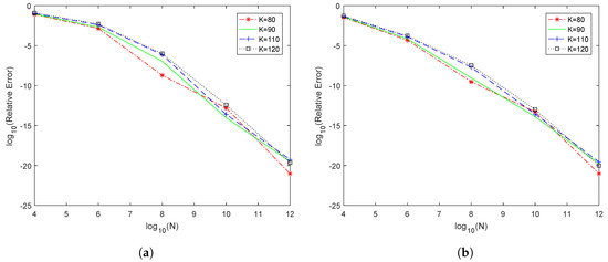
Figure 1. Relative errors with payoff $b\left(s\right)={(s-K)}_{+}$: (a) BS model; (b) Kou model.

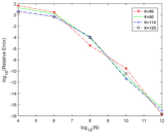
Figure 2. Relative errors for BS model with payoff $b\left(s\right)={(K-s)}_{+}$ and finite expiry time $T=20$.

4.2. The 2D COS Results

In this subsection, the valuation results involving two assets in a GMDB contract are presented. For illustrative purpose, we assumed that the density function of $T_x$ is represented by the combination of exponential distribution Equation (35). Besides, we considered a bivariate normal distribution. In addition, suppose that $(S_1\left(t\right),S_2\left(t\right))$ is a bivariate geometric Brownian motion, where the log-asset price at time t is bivariate normally distributed:

$$(X_1\left(t\right),X_2\left(t\right))\sim \mathcal{N}(\mathbf{\mu },\mathbf{\Sigma }t),$$

where:

$$\mathbf{\mu }=[0.02,-0.005],\mathbf{\Sigma }=[0.04,0.015;0.015,0.09].$$

Set $(S_1\left(0\right),S_2\left(0\right))=(90,110)$, and the strike price $K=100$. We considered the cosine expansion over a symmetric interval $[-100,100]\times [-100,100]$.

In Gerber et al. [3], the valuation equations for GMDB with the exchange option type were explicitly obtained by the Esscher transform, from which we can compute reference values and relative errors. Motivated by the idea in Gerber et al. [3], we further considered some other option types. Approximation results are given in Table 8, and the relative errors confirmed the accuracy of the proposed procedure. It was observed that as N increased, the relative errors decreased.

Table 8. Approximation results for 2D GMDB.

Option Type	$\mathit{N}=2^6$	$\mathit{N}=2^8$	$\mathit{N}=2^{10}$	$\mathit{N}=2^{12}$
Exchange Option	$140.8768$	$153.5866$	$153.6412$	$153.6411$
	(8.31 × ${10}^{-2}$)	(3.55 × ${10}^{-4}$)	(6.38 × ${10}^{-7}$)	(6.74 × ${10}^{-10}$)
Geometric Option	$111.4024$	$114.0135$	$114.0281$	$114.0281$
	(2.30 × ${10}^{-2}$)	(1.29 × ${10}^{-4}$)	(1.54 × ${10}^{-7}$)	(1.27 × ${10}^{-10}$)
Maximum Option	$470.8768$	$483.5866$	$483.6412$	$483.6411$
	(2.64 × ${10}^{-2}$)	(1.12 × ${10}^{-4}$)	(2.03 × ${10}^{-7}$)	(2.14 × ${10}^{-10}$)
Minimum Option	$129.1232$	$116.4134$	$116.3588$	$116.3589$
	(1.10 × ${10}^{-1}$)	(4.68 × ${10}^{-4}$)	(8.43 × ${10}^{-7}$)	(8.90 × ${10}^{-10}$)

5. Conclusions

In this paper, we used the COS method to value GMDB products under a general Lévy framework. When the death benefit payment depended on only one stock fund, we used the 1D COS method to value the products; when it depended on two stock funds, the 2D COS method was used for valuation. Various numerical results illustrated the accuracy and efficiency of the proposed method.

Our COS method can only be used to value GMDB contracts that depend on the terminal value of the stock price; however, we note that some products are also dependent on the running maximum or minimum of the stock price; for example, life-contingent lookback options and barrier options. Hence, we have to develop the COS method or search for another numerical method to solve this problem. We leave this for future research.

References

- Milevsky, M.A.; Posner, S.E. The titanic option: Valuation of the guaranteed minimum death benefit in variable annuities and mutual funds. J. Risk Insur. 2001, 68, 93–128. [Google Scholar] [CrossRef]
- Bauer, D.; Kling, A.; Russ, J. A universal pricing framework for guaranteed minimum benefits in variable annuities. Astin Bull. 2008, 38, 621–651. [Google Scholar] [CrossRef]
- Gerber, H.U.; Shiu, E.S.W.; Yang, H.L. Valuing equity-linked death benefits and other contingent options: A discounted density approach. Insur. Math. Econ. 2012, 51, 73–92. [Google Scholar] [CrossRef]
- Gerber, H.U.; Shiu, E.S.W.; Yang, H.L. Valuing equity-linked death benefits in jump diffusion models. Insur. Math. Econ. 2013, 53, 615–623. [Google Scholar] [CrossRef]
- Siu, C.C.; Yam, S.C.P.; Yang, H.L. Valuing equity-linked death benefits in a regime-switching framework. Astin Bull. 2015, 45, 355–395. [Google Scholar] [CrossRef]
- Dufresne, D. Stochastic life annuities. N. Am. Actuar. J. 2007, 11, 136–157. [Google Scholar] [CrossRef]
- Ko, B.; Ng, A.C.Y. Discussion on “Stochastic Annuities” by Daniel Dufresne, January, 2007. N. Am. Actuar. J. 2007, 11, 170–171. [Google Scholar] [CrossRef]
- Zhang, Z.M.; Yong, Y.D. Valuing guaranteed equity-linked contracts by Laguerre series expansion. J. Comput. Appl. Math. 2019, 357, 329–348. [Google Scholar] [CrossRef]
- Zhang, Z.M.; Yong, Y.D.; Yu, W.G. Valuing equity-linked death benefits in general exponential Lévy models. J. Comput. Appl. Math. 2020. [Google Scholar] [CrossRef]
- Dai, M.; Kwok, Y.K.; Zong, J.P. Guaranteed minimum withdrawal benefit in variable annuities. Math Financ. 2008, 18, 493–667. [Google Scholar] [CrossRef]
- Bélanger, A.C.; Forsyth, P.A.; Labahn, G. Valuing the guaranteed minimum death benefit clause with partial withdrawals. Appl. Math. Financ. 2009, 16, 451–496. [Google Scholar] [CrossRef]
- Kang, B.; Ziveyi, J. Optimal surrender of guaranteed minimum maturity benefits under stochastic volatility and interest rates. Insur. Math. Econ. 2018, 79, 43–56. [Google Scholar] [CrossRef]
- Asmussen, S.; Laub, P.J.; Yang, H.L. Phase-type models in life insurance: Fitting and valuation of equity-linked benefits. Risks 2019, 7, 17. [Google Scholar] [CrossRef]
- Zhou, J.; Wu, L. Valuing equity-linked death benefits with a threshold expense strategy. Insur. Math. Econ. 2015, 62, 79–90. [Google Scholar] [CrossRef]
- Gerber, H.U.; Shiu, E.S.W.; Yang, H.L. Geometric stopping of a random walk and its applications to valuing equity-linked death benefits. Insur. Math. Econ. 2015, 64, 313–325. [Google Scholar] [CrossRef]
- Ulm, E.R. Analytic solution for return of premium and rollup guaranteed minimum death benefit options under some simple mortality laws. Astin Bull. 2008, 38, 543–563. [Google Scholar] [CrossRef]
- Ulm, E.R. Analytic solution for ratchet guaranteed minimum death benefit options under a variety of mortality laws. Insur. Math. Econ. 2014, 58, 14–23. [Google Scholar] [CrossRef]
- Liang, X.Q.; Tsai, C.C.L.; Lu, Y. Valuing guaranteed equity-linked contracts under piecewise constant forces of mortality. Insur. Math. Econ. 2016, 70, 150–161. [Google Scholar] [CrossRef]
- Fan, K.; Shen, Y.; Siu, T.K.; Wang, R.M. Pricing annuity guarantees under a double regime-switching model. Insur. Math. Econ. 2015, 62, 62–78. [Google Scholar] [CrossRef]
- Ignatieva, K.; Song, A.; Ziveyi, J. Pricing and hedging of guaranteed minimum benefits under regime-switching and stochastic mortality. Insur. Math. Econ. 2016, 70, 286–300. [Google Scholar] [CrossRef]
- Hieber, P. Cliquet-style return guarantees in a regime switching Lévy model. Insur. Math. Econ. 2017, 72, 138–147. [Google Scholar] [CrossRef]
- Fang, F.H.; Oosterlee, C.W. A novel pricing method for European options based on Fourier-Cosine series expansions. SIAM J. Sci. Comput. 2008, 31, 826–848. [Google Scholar] [CrossRef]
- Ruijter, M.J.; Oosterlee, C.W. Two-dimensional Fourier Cosine series expansion method for pricing financial options. SIAM J. Sci. Comput. 2012, 34, B642–B671. [Google Scholar] [CrossRef]
- Leitao, Á.; Oosterlee, C.W.; Ortiz-Gracia, L.; Bohte, S.M. On the data-driven COS method. Appl. Math. Comput. 2018, 317, 68–84. [Google Scholar] [CrossRef]
- Chau, K.W.; Yam, S.C.P.; Yang, H. Fourier-cosine method for Gerber-Shiu functions. Insur. Math. Econ. 2015, 61, 170–180. [Google Scholar] [CrossRef]
- Chau, K.W.; Yam, S.C.P.; Yang, H. Fourier-cosine method for ruin probabilities. J. Comput. Appl. Math. 2015, 281, 94–106. [Google Scholar] [CrossRef]
- Zhang, Z.M. Approximation the density of the time to ruin via Fourier-Cosine series expansion. Astin Bull. 2017, 47, 169–198. [Google Scholar] [CrossRef]
- Yang, Y.; Su, W.; Zhang, Z.M. Estimating the discounted density of the deficit at ruin by Fourier cosine series expansion. Stat. Probabil. Lett. 2019, 146, 147–155. [Google Scholar] [CrossRef]
- Wang, Y.Y.; Yu, W.G.; Huang, Y.J.; Yu, X.L.; Fan, H.L. Estimating the expected discounted penalty function in a compound Poisson insurance risk model with mixed premium income. Mathematics 2019, 7, 305. [Google Scholar] [CrossRef]
- Huang, Y.J.; Yu, W.G.; Pan, Y.; Cui, C.R. Estimating the Gerber-Shiu expected discounted penalty function for Lévy risk model. Discrete Dyn. Nat. Soc. 2019, 2019. [Google Scholar] [CrossRef]
- Deng, G.; Dulaney, T.; McCann, C.J.; Yan, M. Efficient valuation of equity-indexed annuities under Lévy processes using Fourier-cosine series. J. Comput. Financ. 2017, 21, 1–27. [Google Scholar]
- Alonso-García, J.; Wood, O.; Ziveyi, J. Pricing and hedging guaranteed minimum withdrawal benefits under a general Lévy ramework using the COS method. Quant. Financ. 2017, 18, 1049–1075. [Google Scholar] [CrossRef]
- Zhang, Z.M.; Yang, H.L.; Yang, H. On a nonparametric estimator for ruin probability in the classical risk model. Scand. Actuar. J. 2014, 2014, 309–338. [Google Scholar] [CrossRef]
- Chan, T.L.R. Efficient computation of European option prices and their sensitivities with the complex Fourier series method. N. Am. J. Econ. Financ. 2019. [Google Scholar] [CrossRef]
- Zhang, Z.M.; Liu, C.L. Nonparametric estimation for derivatives of compound distribution. J. Korean Stat. Soc. 2015, 44, 327–341. [Google Scholar] [CrossRef]
- Have, Z.V.D.; Oosterlee, C.W. The COS method for option valuation under the SABR dynamics. Int. J. Comput. Math. 2018, 95, 444–464. [Google Scholar] [CrossRef]
- Shimizu, Y.; Zhang, Z.M. Estimating Gerber-Shiu functions from discretely observed Lévy driven surplus. Insur. Math. Econ. 2017, 74, 84–98. [Google Scholar] [CrossRef]
- Tour, G.; Thakoor, N.; Khaliq, A.Q.M.; Tangman, D.Y. COS method for option pricing under a regime-switching model with time-changed Lévy processes. Quant. Financ. 2018, 18, 673–692. [Google Scholar] [CrossRef]
- Zhang, Z.M. Estimating the Gerber-Shiu function by Fourier-Sinc series expansion. Scand. Actuar. J. 2017, 2017, 898–919. [Google Scholar] [CrossRef]
- Wang, Y.Y.; Yu, W.G.; Huang, Y.J. Estimating the Gerber-Shiu function in a compound Poisson risk model with stochastic premium income. Discrete Dyn. Nat. Soc. 2019, 2019. [Google Scholar] [CrossRef]
© 2019 by the authors. Licensee MDPI, Basel, Switzerland. This article is an open access article distributed under the terms and conditions of the Creative Commons Attribution (CC BY) license (http://creativecommons.org/licenses/by/4.0/).