The Italian Domination Numbers of Generalized Petersen Graphs P(n,3)

Abstract

An Italian dominating function of G is a function $f:V\left(G\right)\to \{0,1,2\}$, for every vertex v such that $f\left(v\right)=0$, it holds that ${\sum }_{u\in N\left(v\right)}f\left(u\right)\ge 2$. The Italian domination number ${\gamma }_I\left(G\right)$ is the minimum weight of an Italian dominating function on G. In this paper, we determine the exact values of the Italian domination numbers of $P(n,3)$.

1. Introduction

In a graph G with vertex set $V\left(G\right)$ and edge set $E\left(G\right)$, for any $v\in V$, the open neighborhood of a vertex $v\in V$ is a set $\left\{u\right|(u,v)\in E\}$, denoted by $N\left(v\right)$ and the closed neighborhood of a vertex $v\in V$ is $N\left[v\right]=N\left(v\right)\cup \left\{v\right\}$. The degree of a vertex $v\in V$ is $\left|N\right(v\left)\right|$, denoted by $d\left(v\right)$. The minimum (maximum) degree of G is denoted by $\delta$ (△). $C_n$ is a cycle with n vertexes. $G\square H$ is the Cartesian product of two graphs G and H. A set $D\subseteq V$, if for every vertex $v\in V\setminus D$, v is adjacent to a vertex in D, then D is called a dominating set. The minimum cardinality of a domination set of G is called the domination number of G, denoted by $\gamma \left(G\right)$. There are many different types of domination which have been researched extensively. In recent years, Roman domination as one of a variety of dominations has attracted scholars to study it extensively.

Roman domination is originated from the problem of how to develop defense strategies to defend the Roman cities [1]. If the city has a legion or can be defended from neighboring cities, it is safe. The emperor decreed that a city must have two legions to defend it, so that it can still make it safe after sending one of its legions to a neighboring city. Considering the cost, the emperor wanted to station as few legions as possible. A function $f:V\to \{0,1,2\}$ is a Roman dominating function (RDF) [2] if it satisfies the condition that every vertex u with $f\left(u\right)=0$ is adjacent to at least one vertex v with $f\left(v\right)=2$. The value $w_f\left(V\right)={\sum }_{u\in V}f\left(u\right)$ is the weight of an RDF. The Roman domination number is the minimum weight of an RDF, denoted by ${\gamma }_R\left(G\right)$.

Since then, a lot of papers have been published on various aspects of Roman domination [3,4] and many variations [5,6,7]. Italian domination is a new variation of Roman domination.

Italian domination is a generalization of Roman domination introduced by Mustapha Chellali et al. [8], where it is also called Roman {2}-domination; Michael A. Henning et al. [9] named the concept Italian domination. An Italian dominating function (IDF) is a function $f:V\to \{0,1,2\}$ such that for each vertex v with $f\left(v\right)=0$, ${\sum }_{u\in N\left(v\right)}f\left(u\right)\ge 2$. The value of $w_f\left(V\right)={\sum }_{u\in V}f\left(u\right)$ is the weight of an IDF. The Italian domination number is the minimum weight of an IDF on G, denoted as ${\gamma }_I\left(G\right)$.

Italian domination has attracted many researchers. Mustapha Chellali et al. [8] present bounds relating the Italian domination number of a graph to the 2-rainbow domination number. They demonstrate that the Italian domination number is equal to the 2-rainbow domination number for trees and cactus graphs with no even cycles. Michael A. Henning et al. [9] characterize the tree graphs T with $\gamma \left(T\right)+1={\gamma }_I\left(T\right)$, and characterize T with ${\gamma }_I\left(T\right)=2\gamma \left(T\right)$. Zofia Stȩpień et al. [10] prove ${\gamma }_I(C_n\square C_5)=2n$. Zepeng Li et al. [11] obtain the Italian domination numbers of $C_n\square C_3$ and $C_n\square C_4$, where they call it weak {2}-domination number. Some scholars initiate other aspects of Italian domination, such as Abdelkader Rahmouni et al. [12], who study independent Italian domination, Wenjie Fan et al. [13], who study the outer-independent Italian domination number, and Lutz Volkmann [14], who initiates the study of the Italian domatic number in digraphs.

Let $f:V\to \{0,1,2\}$ be an IDF on a graph G, and $(V_0,V_1,V_2)$ be the ordered partition of V induced by f, where $V_i=\left\{v\in V\right|f\left(v\right)=i\}$ and $|V_i|=n_i$, ($i=0,1,2$). Then, there is a one to one correspondence between f and $(V_0,V_1,V_2)$, so we denote $f=(V_0,V_1,V_2)$. The weight of an IDF is the value $w_f\left(V\right)={\sum }_{v\in V}f\left(v\right)=|V_1|+2|V_2|=n_1+2n_2$. A function $f=(V_0,V_1,V_2)$ is a ${\gamma }_I$-function if it is an IDF and $w_f\left(V\right)={\gamma }_I\left(G\right)$.

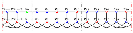
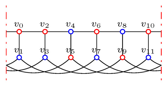
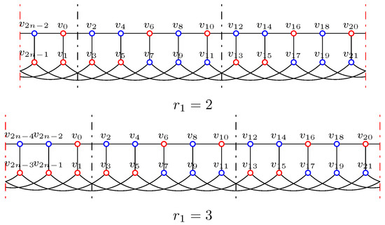
To decide the Italian domination number of a graph is NP-complete, even for bipartite graphs [8]; so it is worthwhile to study the Italian domination numbers for some special classes of graphs. As an interesting family of graphs, various types of domination on generalized Petersen graphs have been studied extensively [15,16,17,18]. For two natural numbers n and k with $n\ge 3$ and $1\le k\le \lfloor \frac{n-1}{2}\rfloor$, the generalized Petersen graph $P(n,k)$ is a graph on $2n$ vertices, $V=\left\{v_i\right|0\le i\le 2n-1\}$ and $E=\{v_i{v}_{i+1},v_i{v}_{i+2}|0\le i\le 2n-1\mathrm{and}i=0(mod2)\}\cup \left\{v_i{v}_{i+2k}\right|0\le i\le 2n-1\mathrm{and}i=1(mod2)\}$, where subscripts are taken modulo n. Figure 1a shows the graph of $P(n,3)$; for convenience and clarity, we always cut the graph $P(n,3)$ between $v_0$ and $v_{2n-2}$, and Figure 1b shows the cut $P(7,3)$.

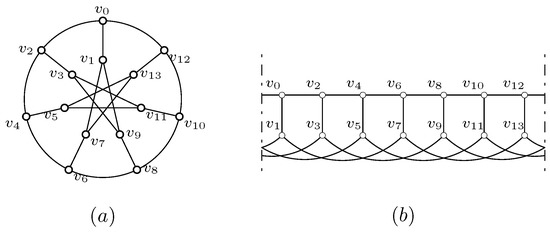
Figure 1. Graphs $P(n,k)$ $(n=7,k=3)$.

While there are many studies on Italian domination, the results of Italian domination on $P(n,3)$ have not been reported. In this paper, the Italian domination number of $P(n,3)$ is studied. We determined the exact value of the Italian domination number on $P(n,3)$.

2. Upper Bounds on the Italian Domination Number of $\mathit{P}(\mathit{n},\mathbf{3})$

The Italian domination number of $P(n,3)$ can be bounded with the 2-rainbow domination number. A 2-rainbow domination function (2RDF) is defined as a function $f:V\to \mathcal{P}\{1,2\}$ such that for every vertex v with $f\left(v\right)=\varnothing$, ${\sum }_{u\in N\left(v\right)}f\left(u\right)=\{1,2\}$. The minimum weight of a 2RDF on G is called the 2-rainbow domination number, denoted as ${\gamma }_{r2}\left(G\right)$.

Lemma 1 ([8]).

For any graph G, then ${\gamma }_I\left(G\right)\le {\gamma }_{r2}\left(G\right)$, where ${\gamma }_{r2}\left(G\right)$ is the 2-rainbow domination number.

Lemma 2 ([15]).

For $n\ge 13$,

$${\gamma }_{r2}\left(P(n,3)\right)\le \left\{\begin{array}{cc}n-⌊\frac{n}{8}⌋,\hfill & n\equiv 0,2,4,5,6,7,13,14,15(mod16),\hfill \\ n-⌊\frac{n}{8}⌋+1,\hfill & otherwise.\hfill \end{array}\right.$$

By Lemma 1 and 2, we can get

Lemma 3.

Let G be a graph $P(n,3)$,

$${\gamma }_I\left(G\right)\le \left\{\begin{array}{cc}n-⌊\frac{n}{8}⌋,\hfill & n\equiv 0,2,4,5,6,7,13,14,15(mod16),\hfill \\ n-⌊\frac{n}{8}⌋+1,\hfill & otherwise.\hfill \end{array}\right.$$

We can get better upper bounds of ${\gamma }_I\left(P(n,3)\right)$ than Lemma 3 by constructing some IDFs. An IDF f on $P(n,3)$ is given as the following;

$$\begin{array}{c}\hfill f=\left(\begin{array}{ccccc}f\left(v_0\right)\hfill & f\left(v_2\right)\hfill & f\left(v_4\right)\hfill & \cdots \hfill & f\left(v_{2n-2}\right)\hfill \\ f\left(v_1\right)\hfill & f\left(v_3\right)\hfill & f\left(v_5\right)\hfill & \cdots \hfill & f\left(v_{2n-1}\right)\hfill \end{array}\right).\end{array}$$

Theorem 1.

Let G be a graph $P(n,3)$,

$${\gamma }_I\left(G\right)\le \left\{\begin{array}{cc}⌈\frac{4n}{5}⌉,\hfill & n\equiv 0,4(mod5)\mathrm{or}n=8,\hfill \\ ⌈\frac{4n}{5}⌉+1,\hfill & \mathrm{otherwise}.\hfill \end{array}\right.$$

Proof. 

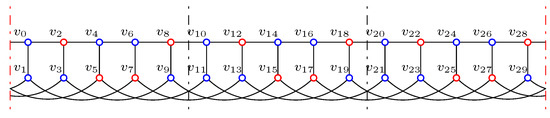
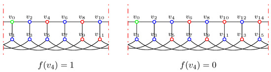
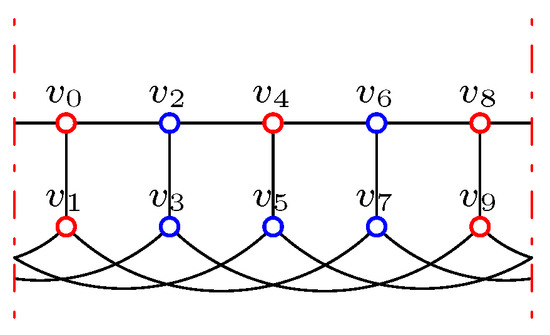
For $n\equiv 0(mod5)$, we construct the function as follows;

$$\begin{array}{c}\hfill f={\left(\begin{array}{ccccc}0\hfill & 1\hfill & 0\hfill & 0\hfill & 1\hfill \\ 0\hfill & 0\hfill & 1\hfill & 1\hfill & 0\hfill \end{array}\right)}^{\frac{n}{5}},\end{array}$$

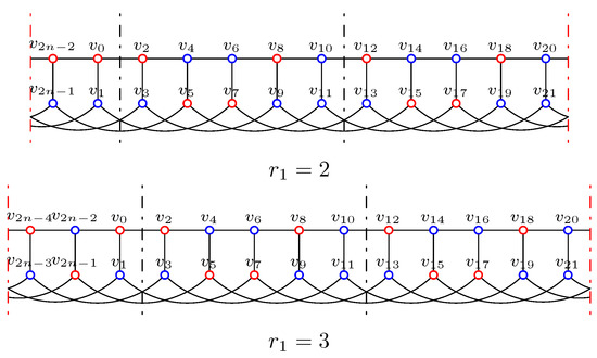
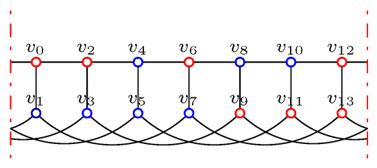
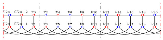
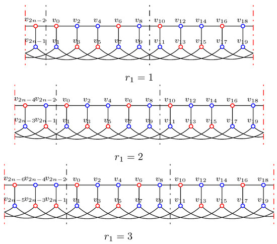
where $\frac{n}{5}$ means we repeat the five columns $\frac{n}{5}$ times. Figure 2 shows f on $P(15,3)$, where red vertices stand for $f\left(v\right)=1$, and blue vertices stand for $f\left(v\right)=0$.

Figure 2. The function f on $P(15,3)$.

By the construction of f, together with Figure 2, one can check f is an IDF. In fact, for $0\le i\le 2n-1$, we can let $i=10m+r$, $m=\lfloor \frac{i}{10}\rfloor$, $r=i(mod10)$, then for $v_i\in V_0$ and $0\le m<\frac{n}{5}$, it has

$$N\left(v_i\right)\cap V_1=\left\{\begin{array}{cc}\{v_{i+2},v_{i-2}\},\hfill & r=0,\hfill \\ \{v_{i-6},v_{i+6}\},\hfill & r=1,\hfill \\ \{v_{i-1},v_{i-6}\},\hfill & r=3,\hfill \\ \{v_{i+1},v_{i-2}\},\hfill & r=4,\hfill \\ \{v_{i+1},v_{i+2}\},\hfill & r=6,\hfill \\ \{v_{i-1},v_{i+6}\},\hfill & r=9,\hfill \end{array}\right.$$

where subscripts are taken modulo $2n$; so ${\sum }_{u\in N\left(v\right)}f\left(u\right)\ge 2$ for every vertex v with $f\left(v\right)=0$, f is an IDF. The weight of f is $f\left(V\right)=\frac{n}{5}\times 4=\frac{4n}{5}$.

Hence, ${\gamma }_I\left(P(n,3)\right)\le \lceil \frac{4n}{5}\rceil$ for $n\equiv 0\left(\mathrm{mod}5\right)$.

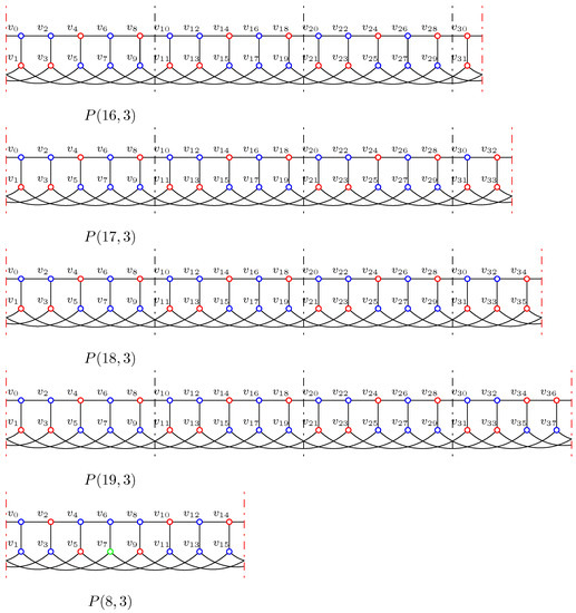
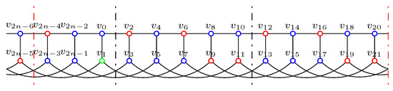
Table 1 shows f and the weight in other cases.

Table 1. f on $P(n,3)$ for $n\ge 1(mod5)$.

n	Function f	Weight of f
$n\equiv 1(mod5)$	$f={\left(\begin{array}{ccccc}0& 0& 1& 0& 1\\ 1& 1& 0& 0& 0\end{array}\right)}^{\frac{n-1}{5}}\left(\begin{array}{c}1\\ 1\end{array}\right)$	$f\left(V\right)=\frac{n-1}{5}\times 4+2=\frac{4n+6}{5}$
$n\equiv 2(mod5)$	$f={\left(\begin{array}{ccccc}0& 0& 1& 0& 1\\ 1& 1& 0& 0& 0\end{array}\right)}^{\frac{n-2}{5}}\left(\begin{array}{cc}0& 1\\ 1& 1\end{array}\right)$	$f\left(V\right)=\frac{n-2}{5}\times 4+3=\frac{4n+7}{5}$
$n\equiv 3(mod5)$$(n\ge 13)$	$f={\left(\begin{array}{ccccc}0& 0& 1& 0& 1\\ 1& 1& 0& 0& 0\end{array}\right)}^{\frac{n-3}{5}}\left(\begin{array}{ccc}0& 0& 1\\ 1& 1& 1\end{array}\right)$	$f\left(V\right)=\frac{n-3}{5}\times 4+4=\frac{4n+8}{5}$
$n\equiv 4(mod5)$	$f={\left(\begin{array}{ccccc}0& 0& 1& 0& 1\\ 1& 1& 0& 0& 0\end{array}\right)}^{\frac{n-4}{5}}\left(\begin{array}{cccc}0& 0& 1& 1\\ 1& 1& 0& 0\end{array}\right)$	$f\left(V\right)=\frac{n-4}{5}\times 4+4=\frac{4n+4}{5}$
$n=8$	$f=\left(\begin{array}{cccccccc}0& 1& 0& 0& 0& 1& 0& 1\\ 0& 0& 1& 2& 1& 0& 0& 0\end{array}\right)$	$f\left(V\right)=7$

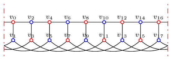
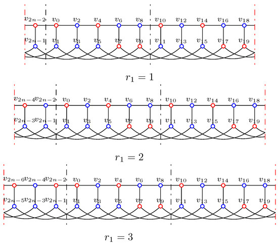
where $\frac{n-i}{5}$ $(i=1,2,3,4)$ means we repeat the leftmost five columns $\frac{n-i}{5}$ times. Figure 3 shows f on $P(n,3)$ $(n=16,17,18,19,8)$, and one can check these functions are IDFs.

Figure 3. The functions f on $P(n,3)$ $(n=16,17,18,19,8)$.

Hence,

$${\gamma }_I\left(G\right)\le \left\{\begin{array}{cc}⌈\frac{4n}{5}⌉,\hfill & n\equiv 0,4(mod5)\mathrm{or}n=8,\hfill \\ ⌈\frac{4n}{5}⌉+1,\hfill & \mathrm{otherwise}.\hfill \end{array}\right.$$

□

3. Lower Bounds on the Italian Domination Number of $\mathit{P}(\mathit{n},\mathbf{3})$

Lemma 4.

Let G be a graph $P(n,3)$, ${\gamma }_I\left(G\right)\ge ⌈\frac{4n}{5}⌉$.

Proof. 

By using Theorem 11 in [8], ${\gamma }_I\left(G\right)\ge \frac{2\left|V\right(G\left)\right|}{\Delta +2}$. In $P(n,3)$, $\Delta =3$, $\left|V\right(G\left)\right|=2n$, so we obtain the lower bound. □

By Theorem 1 and Lemma 4, we can get Theorem 2.

Theorem 2.

For $n\equiv 0,4(mod5)$ and $n=8$, ${\gamma }_I\left(P(n,3)\right)=⌈\frac{4n}{5}⌉$.

Theorem 3.

For $n\equiv 1,2,3(mod5)$ and $n\ne 8$, ${\gamma }_I\left(P(n,3)\right)\ge ⌈\frac{4n}{5}⌉+1$.

In order to prove Theorem 3, we need some definitions, observations and lemmas. Let $f=(V_0,V_1,V_2)$ be an arbitrary IDF of $P(n,3)$, we define functions $g_f$ and $r_f$ as follows.

Definition 1.

For $v\in V\left(G\right)$,

$$g_f\left(v\right)=\left\{\begin{array}{cc}0.2|V_1\cap N\left(v\right)|+0.5|V_2\cap N\left(v\right)|,\hfill & v\in V_0,\hfill \\ 0.4+0.2|V_1\cap N\left(v\right)|+0.5|V_2\cap N\left(v\right)|,\hfill & v\in V_1,\hfill \\ 0.5+0.2|V_1\cap N\left(v\right)|+0.5|V_2\cap N\left(v\right)|,\hfill & v\in V_2.\hfill \end{array}\right.$$

Definition 2.

Define $r_f\left(v\right)=g_f\left(v\right)-0.4$ for $v\in V\left(G\right)$, and $r_f\left(S\right)={\displaystyle \sum _{v\in S}}\left(r_f\left(v\right)\right)$ for $S\subseteq V\left(G\right)$.

By Definition 1 and 2, we have the following observations.

Observation 1.

For any vertex $v\in V\left(G\right)$, $g_f\left(v\right)\ge 0.4$.

Observation 2.

O1

If there exists a vertex v with $v\in V_0$ and $|N\left(v\right)\cap V_1|=2$, then $r_f\left(V\right)\ge 0$.

O2

If there exists a vertex v with $v\in V_0$ and $|N\left(v\right)\cap V_1|=3$, then $r_f\left(V\right)\ge 0.2$.

O3

If there exists a vertex v with $v\in V_2$, then $r_f\left(V\right)\ge 0.4$.

O4

If there exists a pair of vertices $u,v$ with $u,v\in V_1$ and $(u,v)\in E$, then $r_f\left(V\right)\ge 0.4$.

O5

If there exists a vertex v with $v\in V_0$ and $|N\left(v\right)\cap V_0|=|N\left(v\right)\cap V_1|=|N\left(v\right)\cap V_2|=1$, then $r_f\left(V\right)\ge 0.6$.

O6

If there exists a vertex v with $v\in V_0$, $|N\left(v\right)\cap V_1|=2$, and $|N\left(v\right)\cap V_2|=1$, then $r_f\left(V\right)\ge 0.8$.

O7

If there exists a pair of vertices $u,v$ with $u\in V_1$, $v\in V_2$$(oru\in V_2,v\in V_1)$ and $(u,v)\in E$, then $r_f\left(V\right)\ge 1$.

Figure 4 shows O1–O7 in Observation 2 (where red vertices stand for $f\left(v\right)=1$, blue vertices stand for $f\left(v\right)=0,$ and green vertices stand for $f\left(v\right)=2$).

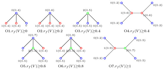
Figure 4. O1–O7.

Lemma 5.

Let $G=(V,E)$; if f is a ${\gamma }_I-function$, then $g_f\left(V\right)={\displaystyle \sum _{v\in V}}{g}_f\left(v\right)={\gamma }_I\left(G\right)$.

Proof. 

$P(n,3)$ is a $3-$regular graph, i.e., $\left|N\right(v\left)\right|=3$ for every vertex $v\in V$. By Definition 1 and definition the of IDF, it has

$$\begin{array}{ccc}{\gamma }_I\left(G\right)\hfill & =\hfill & |V_1|+2|V_2|\hfill \\ & =\hfill & 0.4|V_1|+0.2\times 3|V_1|+0.5|V_2|+0.5\times 3|V_2|\hfill \\ & =\hfill & 0.4|V_1|+0.2{\displaystyle \sum _{v\in V_1}}\left|N\left(v\right)\right|+0.5|V_2|+0.5{\displaystyle \sum _{v\in V_2}}\left|N\left(v\right)\right|\hfill \\ & =\hfill & 0.4|V_1|+0.2{\displaystyle \sum _{v\in V_1}}|N\left(v\right)\cap V_0|+0.2{\displaystyle \sum _{v\in V_1}}|N\left(v\right)\cap V_1|+0.2{\displaystyle \sum _{v\in V_1}}|N\left(v\right)\cap V_2|\hfill \\ & & +0.5|V_2|+0.5{\displaystyle \sum _{v\in V_2}}|N\left(v\right)\cap V_0|+0.5{\displaystyle \sum _{v\in V_2}}|N\left(v\right)\cap V_1|+0.5{\displaystyle \sum _{v\in V_2}}|N\left(v\right)\cap V_2|\hfill \\ & =\hfill & 0.2{\displaystyle \sum _{v\in V_1}}|N\left(v\right)\cap V_0|+0.5{\displaystyle \sum _{v\in V_2}}|N\left(v\right)\cap V_0|\hfill \\ & & +0.4|V_1|+0.2{\displaystyle \sum _{v\in V_1}}|N\left(v\right)\cap V_1|+0.5{\displaystyle \sum _{v\in V_2}}|N\left(v\right)\cap V_1|\hfill \\ & & +0.5|V_2|+0.2{\displaystyle \sum _{v\in V_1}}|N\left(v\right)\cap V_2|+0.5{\displaystyle \sum _{v\in V_2}}|N\left(v\right)\cap V_2|\hfill \\ & =\hfill & {\displaystyle \sum _{v\in V_0}}\left(0.2\right|V_1\cap N\left(v\right)|+0.5|V_2\cap N\left(v\right)\left|\right)\hfill \\ & & +{\displaystyle \sum _{v\in V_1}}(0.4+0.2|V_1\cap N\left(v\right)|+0.5|V_2\cap N\left(v\right)\left|\right)\hfill \\ & & +{\displaystyle \sum _{v\in V_2}}(0.5+0.2|V_1\cap N\left(v\right)|+0.5|V_2\cap N\left(v\right)\left|\right)\hfill \\ & =\hfill & {\displaystyle \sum _{v\in V_0}}{g}_f\left(v\right)+{\displaystyle \sum _{v\in V_1}}{g}_f\left(v\right)+{\displaystyle \sum _{v\in V_2}}{g}_f\left(v\right)\hfill \\ & =\hfill & g_f\left(V\right).\hfill \end{array}$$

□

Lemma 6.

For $n\equiv r_1(mod5)(r_1=1,2,3)$ and $n\ne 8$, let f is a ${\gamma }_I-function$, then

$${\gamma }_I\left(P(n,3)\right)>\lceil \frac{4n}{5}\rceil ⟺r_f\left(V\right)>0.2r_1.$$

Proof. 

By Definition 2 and Lemma 5, $r_f\left(v\right)=g_f\left(v\right)-0.4$, so $r_f\left(V\right)={\gamma }_I\left(G\right)-0.8n$, ${\gamma }_I\left(G\right)=r_f\left(V\right)+0.8n$.

Let $m_1=\lfloor \frac{n}{5}\rfloor ,n=5m_1+r_1$.

$$\begin{array}{ccc}\hfill {\gamma }_I\left(P(n,3)\right)>\lceil \frac{4n}{5}\rceil & ⟺& r_f\left(V\right)+0.8n>\lceil \frac{4n}{5}\rceil \hfill \\ & ⟺& \left\{\begin{array}{c}\begin{array}{ccc}{r}_1=1,\hfill & r_f\left(V\right)\hfill & >⌈\frac{4(5m_1+1)}{5}⌉-\frac{4(5m_1+1)}{5}\hfill \\ & & >4m_1+1-4m_1-\frac{4}{5}\hfill \\ & & >0.2=0.2r_1,\hfill \\ r_1=2,\hfill & r_f\left(V\right)\hfill & >⌈\frac{4(5m_1+2)}{5}⌉-\frac{4(5m_1+2)}{5}\hfill \\ & & >4m_1+2-4m_1-\frac{8}{5}\hfill \\ & & >0.4=0.2r_1,\hfill \\ r_1=3,\hfill & r_f\left(V\right)\hfill & >⌈\frac{4(5m_1+3)}{5}⌉-\frac{4(5m_1+3)}{5}\hfill \\ & & >4m_1+3-4m_1-\frac{12}{5}\hfill \\ & & >0.6=0.2r_1.\hfill \end{array}\hfill \end{array}\right.\hfill \end{array}$$

□

Based on O3, O4, O6 and O7, if one of the conditions in Table 2 appears, then $r_f\left(V\right)>0.2r_1$ ($r_1=1,2,3$).

Table 2. Sufficient conditions for $r_f\left(V\right)>0.2r_1$ ($r_1=1,2,3$).

SC1: $|V_2|\ge 2$.

SC2: $\left|\right(1,1\left)\right|\ge 2$, $(1,1)$ means edges with two endpoints $u,v$ that $u,v\in V_1$.

SC3: $|V_2|+|(1,1)|\ge 2$.

SC4: $\left|\right(1,2\left)\right|\ge 1$, $(1,2)$ means edges with two endpoints $u,v$ that $u\in V_1$ and $v\in V_2$.

SC5: ∃$v\in V_0$ with $|N\left(v\right)\cap V_1|=2$ and $|N\left(v\right)\cap V_2|=1$.

In fact, $r_f\left(V\right)>0.2r_1$ $(r_1=1,2,3)$ is always true; so, besides these sufficient conditions, the following cases need to be considered:

(1)

$|V_2|=1$.

(2)

$\left|\right(1,1\left)\right|=1$.

(3)

∃$v\in V_0$ with $|N\left(v\right)\cap V_1|=3$.

(4)

Excluding these sufficient conditions and cases (1)–(3), then $|V_2|=0$, $\left|\right(1,1\left)\right|=0$, and $v\in V_0$, $|N\left(v\right)\cap V_1|\le 2$. In this case, by the definition of IDF, for $i(mod2)=0$, $\exists v_i$, $f\left(v_i\right)=1$.

In the sequel, we will prove $r_f\left(V\right)>0.2r_1$ $(r_1=1,2,3)$ in the above four cases by Lemmas 7–10.

Lemma 7.

If there is a vertex v with $v\in V_2$, then $r_f\left(V\right)>0.2r_1$ $(r_1=1,2,3)$.

Proof. 

Suppose $f\left(v_0\right)=2$ or $f\left(v_1\right)=2$.

For $r_1=1$, by O3, $r_f\left(V\right)>0.2r_1$.

For $r_1=2,3$, by contrast, suppose $r_f\left(V\right)\le 0.2r_1$.

Case 1.$f\left(v_0\right)=2$. By excluding $\mathbf{SC}\mathbf{1}$, $f\left(v_i\right)\ne 2$ for $1\le i\le 2n-1$.

By excluding $\mathbf{SC}\mathbf{4}$, $f\left(v_1\right)=f\left(v_2\right)=0$. Then, $f\left(v_3\right)=1$ or 0.

Case 1.1.$f\left(v_3\right)=1$. By O5, $r_f\left(V\right)\ge 0.6$, $r_1=3$.

By excluding $\mathbf{SC}\mathbf{5}$, $f\left(v_4\right)=0$. By the definition of IDF, $f\left(v_5\right)=1$, $f\left(v_6\right)=1$.

By excluding $\mathbf{SC}\mathbf{3}$, $f\left(v_7\right)=f\left(v_8\right)=f\left(v_9\right)=0$. By the definition of IDF, $f\left(v_{10}\right)=1$.

By excluding $\mathbf{SC}\mathbf{3}$, $f\left(v_{11}\right)=f\left(v_{12}\right)=0$.

Continuing in this way, it has

$f\left(v_i\right)=1$, $v_i\in V$ and $i\in \{10m+3,10m+5,10m+6,10m+10\}$.

$f\left(v_i\right)=0$, $v_i\in V$ and $i\in \{10m+2,10m+4,10m+7,10m+8,10m+9,10m+11\}$.

Since $r_1=3$, $n=5m_1+r_1=5m_1+3$, $2n-1=10m_1+5$, then $v_{2n-1},v_5\in V_1$ and $(v_{2n-1},v_5)\in E$, by $\mathbf{O}3$–$\mathbf{O}4$, $r_f\left(V\right)\ge 0.8>0.2r_1$, a contradiction.

Figure 5 shows the segment of f, where red vertices stand for $f\left(v\right)=1$, blue vertices stand for $f\left(v\right)=0$ and green vertices stand for $f\left(v\right)=2$.

Figure 5. Segment of f in case 1.1 in Lemma 7.

Case 1.2.$f\left(v_3\right)=0$. By excluding $\mathbf{SC}\mathbf{1}$, $f\left(v_4\right)=1$ or 0.

Case 1.2.1.$f\left(v_4\right)=1$. By O5, $r_f\left(V\right)\ge 0.6$, $r_1=3$.

By excluding $\mathbf{SC}\mathbf{3}$, $f\left(v_5\right)=f\left(v_6\right)=0$.

Next, $f\left(v_7\right)=1$ or 0. If $f\left(v_7\right)=1$, then $f\left(v_2\right)=f\left(v_1\right)=0$, and $|N\left(v_2\right)\cap V_1|=1$, $|N\left(v_2\right)\cap V_2|=1$, $|N\left(v_1\right)\cap V_1|=1$, $|N\left(v_1\right)\cap V_2|=1$, by O5, $r_f\left(V\right)\ge 1.2>0.2r_1$, a contradiction; so $f\left(v_7\right)=0$.

By the definition of IDF, $f\left(v_8\right)=f\left(v_9\right)=1$. Then $v_8,v_9\in V_1$ and $(v_8,v_9)\in E$, by $\mathbf{O}3$ and $\mathbf{O}4$, $r_f\left(V\right)\ge 0.8>0.2r_1$, a contradiction. Figure 6 (left) shows the segments of f.

Figure 6. Segments of f in case 1.2 in Lemma 7.

Case 1.2.2.$f\left(v_4\right)=0$.

By the definition of IDF, $f\left(v_5\right)=f\left(v_6\right)=f\left(v_9\right)=1$. By excluding $\mathbf{SC}\mathbf{3}$, $f\left(v_7\right)=f\left(v_8\right)=0$.

By excluding $\mathbf{SC}\mathbf{3}$, $f\left(v_{11}\right)=f\left(v_{15}\right)=0$. By the definition of IDF, $f\left(v_{10}\right)=f\left(v_{13}\right)=1$.

By excluding $\mathbf{SC}\mathbf{3}$, $f\left(v_{12}\right)=0$. By the definition of IDF, $f\left(v_{14}\right)=1$.

Then, $|N\left(v_8\right)\cap V_1|=3$ and $|N\left(v_{12}\right)\cap V_1|=3$, by O2 and O3, $r_f\left(V\right)\ge 0.8>0.2r_1$, a contradiction. Figure 6 (right) shows the segments of f.

Case 2.$f\left(v_1\right)=2$. By excluding $\mathbf{SC}\mathbf{1}$, $f\left(v_i\right)\ne 2$ for $0\le i\le 2n-1$ and $i\ne 1$.

By excluding $\mathbf{SC}\mathbf{4}$, $f\left(v_0\right)=f\left(v_7\right)=0$. Then, $f\left(v_2\right)=1$ or 0.

Case 2.1.$f\left(v_2\right)=1$. By O5, $r_f\left(V\right)\ge 0.6$, $r_1=3$.

By excluding $\mathbf{SC}\mathbf{3}$, $f\left(v_3\right)=f\left(v_4\right)=0$. By the definition of IDF, $f\left(v_6\right)=1$.

Next, $f\left(v_5\right)=1$ or 0. If $f\left(v_5\right)=1$, then $|N\left(v_0\right)\cap V_1|=1$, $|N\left(v_0\right)\cap V_2|=1$, $|N\left(v_4\right)\cap V_1|=3$, by O2 and O5, $r_f\left(V\right)\ge 0.8>0.2r_1$, a contradiction. So, $f\left(v_5\right)=0$.

By the definition of IDF, $f\left(v_{11}\right)=1$. By excluding $\mathbf{SC}\mathbf{3}$, $f\left(v_8\right)=f\left(v_{10}\right)=0$.

By the definition of IDF, $f\left(v_9\right)=f\left(v_{12}\right)=1$.

Continuing in this way, it has

$f\left(v_i\right)=1$, $v_i\in V$ and $i\in \{10m+2,10m+6,10m+9,10m+11\}$,

$f\left(v_i\right)=0$, $v_i\in V$ and $i\in \{10m+3,10m+4,10m+5,10m+7,10m+8,10m+10\}$.

Since $r_1=3$, $n=5m_1+r_1=5m_1+3$, $2n-5=10m_1+1$, then $v_{2n-5}\in V_1,v_1\in V_2$ and $(v_{2n-5},v_1)\in E$, by O7, $r_f\left(V\right)\ge 1>0.2r_1$, a contradiction. Figure 7 shows the segment of f.

Figure 7. Segment of f in case 2.1 in Lemma 7.

Case 2.2.$f\left(v_2\right)=0$.

By the definition of IDF, $f\left(v_3\right)=f\left(v_4\right)=1$. By excluding $\mathbf{SC}\mathbf{3}$, $f\left(v_5\right)=f\left(v_6\right)=f\left(v_9\right)=0$.

By excluding $\mathbf{SC}\mathbf{4}$, $f\left(v_7\right)=0$. By the definition of IDF, $f\left(v_8\right)=1$.

By excluding $\mathbf{SC}\mathbf{3}$, $f\left(v_{10}\right)=0$. By the definition of IDF, $f\left(v_{11}\right)=1$.

Next, $f\left(v_{12}\right)=1$ or 0.

Case 2.2.1.$f\left(v_{12}\right)=1$. Then, $|N\left(v_{10}\right)\cap V_1|=3$, by O2 and O3, $r_f\left(V\right)\ge 0.6$, $r_1=3$.

By excluding $\mathbf{SC}\mathbf{3}$, $f\left(v_{13}\right)=f\left(v_{14}\right)=0$. By the definition of IDF, $f\left(v_{15}\right)=1$.

Then $|N\left(v_9\right)\cap V_1|=3$ and $|N\left(v_{10}\right)\cap V_1|=3$, by O2 and O3, $r_f\left(V\right)\ge 0.8>0.2r_1$, a contradiction. Figure 8 (above) shows the segment of f.

Figure 8. Segments of f in case 2.2 in Lemma 7.

Case 2.2.2.$f\left(v_{12}\right)=0$.

By the definition of IDF, $f\left(v_{13}\right)=f\left(v_{14}\right)=1$.

By excluding $\mathbf{SC}\mathbf{3}$, $f\left(v_{15}\right)=f\left(v_{16}\right)=f\left(v_{17}\right)=f\left(v_{19}\right)=0$.

By the definition of IDF, $f\left(v_{18}\right)=f\left(v_{21}\right)=1$. By excluding $\mathbf{SC}\mathbf{3}$, $f\left(v_{20}\right)=0$.

Continuing in this way, it has

$f\left(v_i\right)=1,i\in \{10m+3,10m+4,10m+8,10m+11\}$,

$f\left(v_i\right)=0,i\in \{10m+2,10m+5,10m+6,10m+7,10m+9,10m+10\}$.

For $r_1=2$, $|N\left(v_7\right)\cap V_1|=1$ and $|N\left(v_7\right)\cap V_2|=1$, by O5, $r_f\left(V\right)\ge 0.6>0.2r_1$, a contradiction.

For $r_1=3$, $n=5m_1+r_1=5m_1+3$, $2n-3=10m_1+3$, then $v_{2n-3}\in V_1$, $v_3\in V_1$, $(v_{2n-3},v_3)\in E$, by O3–O4, $r_f\left(V\right)\ge 0.8>0.2r_1$, a contradiction. Figure 8 (below) shows the segment of f.

 □

Lemma 8.

If there exists a pair of vertices $u,v$ with $u,v\in V_1$ and $(u,v)\in E$, then $r_f\left(V\right)>0.2r_1$ $(r_1=1,2,3)$.

Proof. 

Without loss of generality, let $f\left(v_0\right)=f\left(v_2\right)=1$ or $f\left(v_0\right)=f\left(v_1\right)=1$ or $f\left(v_1\right)=f\left(v_7\right)=1.$

For $r_1=1$, by O4, $r_f\left(V\right)\ge 0.4>0.2r_1$.

For $r_1=2,3$, by contrast, suppose $r_f\left(V\right)\le 0.2r_1$. Similar to Lemma 7, by excluding the sufficient conditions in Table 2 and Lemma 7, and by the definition of IDF, we can get the values of each vertex step by step.

Case 1.$f\left(v_0\right)=f\left(v_2\right)=1$. After that, $f\left(v_1\right)=f\left(v_3\right)=f\left(v_4\right)=0$, and $f\left(v_5\right)=1$ or 0.

Case 1.1.$f\left(v_5\right)=1$. Then, $f\left(v_6\right)=1$ or 0.

Case 1.1.1.$f\left(v_6\right)=1$. Afterwards, $f\left(v_7\right)=f\left(v_8\right)=f\left(v_{11}\right)=0$, $f\left(v_9\right)=f\left(v_{10}\right)=1$. Then $|N\left(v_4\right)\cap V_1|=3$ and $|N\left(v_8\right)\cap V_1|=3$, by O2 and O4, $r_f\left(V\right)\ge 0.8>0.2r_1$, a contradiction. Figure 9 shows the segment of f.

Figure 9. Segment of f in case 1.1.1 in Lemma 8.

Case 1.1.2.$f\left(v_6\right)=0$. Then, it has

$f\left(v_i\right)=1$, $i\in \{10m+2,10m+5,10m+7,10m+8\}$,

$f\left(v_i\right)=0$, $i\in \{10m+3,10m+4,10m+6,10m+9,10m+10,10m+11\}$.

For $r_1=2$, $n=5m_1+r_1=5m_1+2$, $2n-2=10m_1+2$, then $v_{2n-2}\in V_1$, $v_0\in V_1$, and $(v_{2n-2},v_0)\in E$, by O4, $r_f\left(V\right)\ge 0.8>0.2r_1$, a contradiction.

For $r_1=3$, $n=5m_1+r_1=5m_1+3$, $2n-1=10m_1+5$, then $v_{2n-1}\in V_1$, $v_5\in V_1$, and $(v_{2n-1},v_5)\in E$, by O4, $r_f\left(V\right)\ge 0.8>0.2r_1$, a contradiction. Figure 10 shows the segments of f.

Figure 10. Segments of f in case 1.1.2 in Lemma 8.

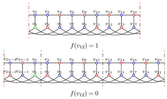
Case 1.2.$f\left(v_5\right)=0$. After that, we can get the values of $f\left(v_i\right)$$(i=6,7,\cdots ,13)$. Figure 11 shows the segment of f. Since $v_{12},v_{13}\in V_1$ and $(v_{12},v_{13})\in E$, by O4, $r_f\left(V\right)\ge 0.8>0.2r_1$.

Figure 11. Segment of f in case 1.2 in Lemma 8.

Case 2.$f\left(v_0\right)=f\left(v_1\right)=1$. Afterwards, $f\left(v_2\right)=0$, $f\left(v_3\right)=1$ or 0.

Case 2.1.$f\left(v_3\right)=1$. After that, $f\left(v_4\right)=1$ or 0.

Case 2.1.1.$f\left(v_4\right)=1$. Then, it has

$f\left(v_i\right)=1$, $i\in \{10m+3,10m+4,10m+8,10m+11\}$,

$f\left(v_i\right)=0$, $i\in \{10m+2,10m+5,10m+6,10m+7,10m+9,10m+10\}$.

For $r_1=2$, $|N\left(v_2\right)\cap V_1|=3$, by O2 and O4, $r_f\left(V\right)\ge 0.6>0.2r_1$, a contradiction.

For $r_1=3$, $v_{2n-2},v_0\in V_1$ and $(v_{2n-2},v_0)\in E$, by O4, $r_f\left(V\right)\ge 0.8>0.2r_1$, a contradiction. Figure 12 shows the segment of f.

Figure 12. Segment of f in case 2.1.1 in Lemma 8.

Case 2.1.2.$f\left(v_4\right)=0$. Then, it has

$f\left(v_i\right)=1$, $i\in \{10m+3,10m+5,10m+6,10m+10\}$,

$f\left(v_i\right)=0$, $i\in \{10m+2,10m+4,10m+7,10m+8,10m+9,10m+11\}$.

For $r_1=2$, $f\left(v_{2n-2}\right)=0$, $f\left(v_{2n-4}\right)=f\left(v_{2n-1}\right)=1$, then $|N\left(v_{2n-2}\right)\cap V_1|=3$, by O2 and O4, $r_f\left(V\right)\ge 0.6>0.2r_1$, a contradiction.

For $r_1=3$, $f\left(v_{2n-3}\right)=1$, then $v_{2n-3},v_3\in V_1$ and $(v_{2n-3},v_3)\in E$, by O4, $r_f\left(V\right)\ge 0.8>0.2r_1$, a contradiction. Figure 13 shows the segments of f.

Figure 13. Segments of f in case 2.1.2 in Lemma 8.

Case 2.2.$f\left(v_3\right)=0$. Afterwards, $f\left(v_4\right)=1$, $f\left(v_5\right)=f\left(v_6\right)=f\left(v_7\right)=0$, $f\left(v_8\right)=f\left(v_9\right)=1$, then $(v_8,v_9)\in E,$$v_8,v_9\in V_1$, by O4, $r_f\left(V\right)\ge 0.8>0.2r_1$, a contradiction. Figure 14 shows the segment of f.

Figure 14. Segment of f in case 2.2 in Lemma 8.

Case 3.$f\left(v_1\right)=f\left(v_7\right)=1$. Then, it has

$f\left(v_i\right)=0$, $i\in \{10m+3,10m+4,10m+6,10m+9,10m+10,10m+11\}$,

$f\left(v_i\right)=1$, $i\in \{10m+2,10m+5,10m+7,10m+8\}$.

For $r_1=2$, $f\left(v_{2n-2}\right)=1$, then $|N\left(v_0\right)\cap V_1|=3$, by O2 and O4, $r_f\left(V\right)\ge 0.6>0.2r_1$, a contradiction.

For $r_1=3$, $f\left(v_{2n-1}\right)=1$, then $v_{2n-1},v_5\in V_1$ and $(v_{2n-1},v_5)\in E$, by O4, $r_f\left(V\right)\ge 0.8>0.2r_1$, a contradiction. Figure 15 shows the segments of f for $r_1=2$ and $r_1=3$.

Figure 15. Segments of f in case 3 in Lemma 8.

 □

Lemma 9.

If there exists a vertex v with $v\in V_0$ and $|N\left(v\right)\cap V_1|=3$, then $r_f\left(V\right)>0.2r_1$ $(r_1=1,2,3)$.

Proof. 

Without loss of generality, it is assumed that $f\left(v_0\right)=f\left(v_3\right)=f\left(v_4\right)=1$ and $f\left(v_2\right)=0$.

Similar to Lemma 7, by excluding the sufficient conditions in Table 2 and Lemma 7 and 8, and by the definition of IDF, we can get the values of each vertex step by step.

Figure 16 shows the values of $f\left(v_i\right)$$(i=5,6,\cdots ,17)$. Then, $|N\left(v_2\right)\cap V_1|=3$, $|N\left(v_6\right)\cap V_1|=3$, $|N\left(v_{10}\right)\cap V_1|=3$ and $|N\left(v_{14}\right)\cap V_1|=3$, by O2, $r_f\left(V\right)\ge 0.8>0.2r_1$ for $r_1=1,2,3$.

Figure 16. Segment of f in Lemma 9.

 □

Lemma 10.

If there exists $v_i$, $f\left(v_i\right)=1$ and $i(mod2)=0$, then $r_f\left(V\right)>0.2r_1$ $(r_1=1,2,3)$.

Proof. 

Without loss of generality, let $f\left(v_0\right)=1$. By contrast, suppose $r_f\left(V\right)\le 0.2r_1$. Similar to Lemma 7, by excluding the sufficient conditions in Table 2 and Lemmas 7–9, and by the definition of IDF, we can get the values of each vertex step by step.

Next, $f\left(v_1\right)=f\left(v_2\right)=0$, $f\left(v_3\right)=1$ or 0.

Case1. $f\left(v_3\right)=1$. Then, it has

$f\left(v_i\right)=1$, $i\in \{10m,10m+3,10m+5,10m+6\}$,

$f\left(v_i\right)=0$, $i\in \{10m+1,10m+2,10m+4,10m+7,10m+8,10m+9\}$.

For $r_1=1$, $f\left(v_{2n-2}\right)=1$, then $v_0,v_{2n-2}\in V_1$ and $(v_0,v_{2n-2})\in E$, by O4, $r_f\left(V\right)\ge 0.4>0.2r_1$, a contradiction.

For $r_1=2$, $f\left(v_{2n-2}\right)=0$, $f\left(v_{2n-1}\right)=f\left(v_{2n-4}\right)=1$, then $v_{2n-1},v_5\in V_1$, $(v_{2n-1},v_5)\in E$ and $|N\left(v_{2n-2}\right)\cap V_1|=3$, by O2 and O4, $r_f\left(V\right)\ge 0.6>0.2r_1$, a contradiction.

For $r_1=3$, $f\left(v_{2n-3}\right)=f\left(v_{2n-1}\right)=1$, then $v_{2n-1},v_5,v_{2n-3},v_3\in V_1$, and $(v_{2n-3},v_3)$, $(v_{2n-1},v_5)\in E$, by O4, $r_f\left(V\right)\ge 0.8>0.2r_1$, a contradiction. Figure 17 shows the segments of f in this case.

Figure 17. Segments of f in case 1 in Lemma 10.

Case2. $f\left(v_3\right)=0$. Then, it has

$f\left(v_i\right)=1$, $i\in \{10m,10m+4,10m+7,10m+9\}$,

$f\left(v_i\right)=0$, $i\in \{10m+1,10m+2,10m+3,10m+5,10m+6,10m+8\}$.

For $r_1=1$, $f\left(v_{2n-2}\right)=1$, then $v_{2n-2},v_0\in V_1$ and $(v_{2n-2},v_0)\in E$, by O4, $r_f\left(V\right)\ge 0.4>0.2r_1$, a contradiction.

For $r_1=2$, $f\left(v_{2n-1}\right)=0$, then $N\left(v_{2n-1}\right)\cap V_0=\{v_{2n-2},v_5\}$, by the definition of IDF, this case can not exist.

For $r_1=3$, $f\left(v_{2n-3}\right)=f\left(v_{2n-4}\right)=0$, then $N\left(v_{2n-3}\right)\cap V_0=\{v_{2n-4},v_3\}$, by the definition of IDF, this case can not exist. Figure 18 shows the segments of f in this case.

Figure 18. Segments of f in case 2 in Lemma 10.

 □

By Lemmas 7–10 and the sufficient conditions in Table 2, we can get that for $n\equiv r_1(mod5)(r_1=1,2,3)$, $r_f\left(V\right)>0.2r_1$, i.e., ${\gamma }_I\left(P(n,3)\right)>\lceil \frac{4n}{5}\rceil$. That is, Theorem 3 holds.

By Theorems 1 and 3, we can obtain

Theorem 4.

For $n\equiv 1,2,3(mod5)$ and $n\ne 8$,

$${\gamma }_I\left(P(n,3)\right)=⌈\frac{4n}{5}⌉+1.$$

By Theorems 2 and 4, we have

Theorem 5.

Let G be a graph $P(n,3)$,

$${\gamma }_I\left(G\right)=\left\{\begin{array}{cc}⌈\frac{4n}{5}⌉,\hfill & n\equiv 0,4(mod5)\mathrm{or}n=8,\hfill \\ ⌈\frac{4n}{5}⌉+1,\hfill & otherwise.\hfill \end{array}\right.$$

References

- Henning, M.A.; Hedetniemi, S.T. Defending the Roman empire—A new strategy. Discret. Math. 2003, 266, 239–251. [Google Scholar] [CrossRef]
- Cockayne, E.J.; Dreyer, P.A.; Hedetniemi, S.M.; Hedetniemi, S.T. Roman domination in graphs. Discret. Math. 2004, 278, 11–22. [Google Scholar] [CrossRef]
- Henning, M.A.; Klostermeyer, W.F.; MacGillivray, G. Perfect Roman domination in trees. Discret. Appl. Math. 2018, 236, 235–245. [Google Scholar] [CrossRef]
- Volkmann, L. Signed total Roman domination in graphs. J. Comb. Optim. 2016, 32, 855–871. [Google Scholar] [CrossRef]
- Shao, Z.H.; Wu, P.; Jiang, H.Q.; Li, Z.P.; Žerovnik, J.; Zhang, X.J. Discharging approach for double Roman domination in graphs. IEEE Access 2018, 6, 63345–63351. [Google Scholar] [CrossRef]
- Ahangar, H.A.; Chellali, M.; Sheikholeslami, S.M. Signed double Roman domination in graphs. Discret. Appl. Math. 2019, 257, 1–11. [Google Scholar] [CrossRef]
- Jiang, H.Q.; Wu, P.; Shao, Z.H.; Rao, Y.S.; Liu, J.B. The double Roman domination numbers of generalized Petersen graphs P (n,2). Mathematics 2018, 6, 206. [Google Scholar] [CrossRef]
- Chellali, M.; Haynes, T.W.; Hedetniemi, S.T.; McRae, A.A. Roman {2}-domination. Discret. Appl. Math. 2016, 204, 22–28. [Google Scholar] [CrossRef]
- Henning, M.A.; Klostermeyer, W.F. Italian domination in trees. Discret. Appl. Math. 2017, 217, 557–564. [Google Scholar] [CrossRef]
- Stȩpień, Z.; Szymaszkiewicz, A.; Szymaszkiewicz, L.; Zwierzchowski, M. 2-Rainbow domination number of Cn□C5. Discret. Appl. Math. 2014, 170, 113–116. [Google Scholar] [CrossRef]
- Li, Z.; Shao, Z.H.; Xu, J. Weak {2}-domination number of Cartesian products of cycles. J. Comb. Optim. 2018, 35, 75–85. [Google Scholar] [CrossRef]
- Rahmouni, A.; Chellali, M. Indenpendent Roman 2-domination in graphs. Discret. Appl. Math. 2018, 236, 408–414. [Google Scholar] [CrossRef]
- Fan, W.J.; Ye, A.S.; Miao, F.; Shao, Z.H.; Samodivkin, V.; Sheikholeslami, S.M. Outer-independent Italian domination in graphs. IEEE Access 2019, 7, 22756–22762. [Google Scholar] [CrossRef]
- Volkmann, L. The Italian domatic number of a digraph. Commun. Comb. Optim. 2019, 4, 61–70. [Google Scholar]
- Xu, G.J. 2-rainbow domination in generalized petersen graph P (n,3). Discret. Appl. Math. 2009, 157, 2570–2573. [Google Scholar] [CrossRef]
- Tong, C.L.; Lin, X.H.; Yang, Y.S.; Luo, M.Q. 2-rainbow domination of generalized Petersen graphs P (n,2). Discret. Appl. Math. 2009, 157, 1932–1937. [Google Scholar] [CrossRef]
- Fu, X.L.; Yang, Y.S.; Jiang, B.Q. On the domination number of generalized Petersen graphs P (n,3). Ars Comb. 2007, 84, 373–383. [Google Scholar]
- Shao, Z.H.; Jiang, H.Q.; Wu, P.; Wang, S.H.; Zerovnik, J.; Zhang, X.S.; Liu, J.B. On 2-rainbow domination of generalized Petersen graphs. Discret. Appl. Math. 2019, 257, 370–384. [Google Scholar] [CrossRef]
© 2019 by the authors. Licensee MDPI, Basel, Switzerland. This article is an open access article distributed under the terms and conditions of the Creative Commons Attribution (CC BY) license (http://creativecommons.org/licenses/by/4.0/).