Credit Risk Contagion and Systemic Risk on Networks

Abstract

This paper proposes a model of the dynamics of credit contagion through non-performing loans on financial networks. Credit risk contagion is modeled in the context of the classical SIS (Susceptibles-Infected-Susceptibles) epidemic processes on networks but with a fundamental novelty. In fact, we assume the presence of two different classes of infected agents, and then we differentiate the dynamics of assets subject to idiosyncratic risk from those affected by systemic risk by adopting a SIIS (Susceptible-Infected1-Infected2-Susceptible) model. In the recent literature in this field, the effect of systemic credit risk on the performance of the financial network is a hot topic. We perform numerical simulations intended to explore the roles played by two different network structures on the long-term behavior of assets affected by systemic risk in order to analyze the effect of the topology of the underlying network structure on the spreading of systemic risk on the structure. Random graphs, i.e., the Erdös–Rényi model, are considered “benchmark” network structures while core-periphery structures are often indicated in the literature as idealized structures, although they are able to capture interesting, specific features of real-world financial networks. Moreover, as a matter of comparison, we also perform numerical experiments on small-world networks.

1. Introduction

Network modeling in social and economic processes, either analytical- or simulation-based, has demonstrated its importance in scientific literature produced in the last two decades (see [1,2] for a general review of related theory, methods, and applications), and the analysis of the emergence of complex and heterogeneous connectivity patterns in many sociotechnical systems has been a hot topic in recent years (see [3] and references therein). Moreover, in the context of complex networks, the study of processes of epidemic spreading plays a crucial role (see [3] for an interesting review of the literature).

Recently, different macroprudential policies involving the analysis and control of credit risk have been based on network models [4,5], and the main point is, basically, the assessment of financial risk by focusing on key structural vulnerabilities that may expose the system to significant stress. Indeed, modeling the credit risk on networks defined by economic interactions in a coherent yet applicable manner is an important yet challenging problem. In fact, as usual, in many real-world problems, it is a typical multi-scale problem, ranging from the level of the credit portfolio of a single financial institution to a complex network of interacting clusters. Techniques coming from network theory have been applied in recent years to model the financial systemic risk correlated with the phenomenon of contagion. These techniques have shown interesting potential in assessing key features of dynamics, basically with the aim of assessing whether the application of complex system methods may allow the anticipation, avoidance, or mitigation of the spreading of systemic credit risk.

In this paper, we propose a model in which each financial institution representing a node of a financial network is modeled as a portfolio of risky assets. The impact of the structure and diversification of financial institutions’ portfolios is very well known. Indeed, a shock is more likely to lead to failure of the institution if its asset concentration is high. One of the main focuses of our work is based on the simple observation that the susceptibility of the system to shocks is likely to be affected more when the asset and liability portfolios of the other institutes in the complex network of interactions are more alike. The main goals introduced here are to explore resilience of the structure to systemic risk and to fully understand the functioning of the banking system as a balance between competitiveness and stability [6,7,8]. Both analyses aim to exploit the role of potential regulations in reducing systemic risks, remembering that competition in banking is important, because any misbehavior has implications on economic growth. In the scientific literature in this field, authors are concerned with the effect of complexity plus homogeneity, which often does not allow stability; on the contrary, it may lead to fragility. Moreover, connectivity may enhance risk dispersion. To address this issue, we exploit numerical simulations to explore the role of connectivity. Basically, numerical simulations are designed to compare the spread of contagion of non-performing loans on a random network characterized by different levels of connection probability, i.e., a level of connectivity ranging from low to high and on core-periphery networks with different ratios between the core and periphery nodes. The core-periphery network structure is chosen because of its representativeness of most real financial networks (see [9,10] for some recent contributions to the scientific literature).

As stated in a recent paper [11], the use of random graphs is motivated by the unobservable nature of real-world financial networks. Since the underlying financial network cannot be observed exactly, a probabilistic framework is needed.

The network approach enables one to use the self-organizing, adaptive nature of such systems. We attempt to analyze the extent of the underlying network structure on the level of systemic risk.

The paper is organized as follows. In Section 2 we introduce credit risk by discussing the probability density function of credit losses. Moreover, we discuss the Vasicek model which provides the basis of the fundamental regulatory laws [12]. In Section 3, we model an interbank network affected by systemic and idiosyncratic risks, where the initial condition for each node, i.e., for each bank in the network, depends on each individual asset structure. We explore the contagion dynamics over different networks’ architectures with the main goal being to understand the impact of the network structure on the systematic part and on the idiosyncratic part of the risk in the Vasicek loan portfolio value model. Linkages among financial institutions represent, in the context of our model, credit swaps. The spreading of risk in the network is modeled in the framework of epidemic processes in complex networks [3] with the novelty, with respect to other models in the related literature, of having split credits between a group subject to systemic risk and another subject to idiosyncratic risk, following the Vasicek model. Section 4 is devoted to some numerical experiments aimed at analyzing the dynamics of systemic risk on different topological structures of networks. Finally, a short section of concluding remarks closes the paper.

2. Credit Risk

Credit risk is considered a fundamental variable due to the fact that it is more directly related to financial stability than other variables. In the following text, we introduce the Vasicek model, which is the most widely used model to calculate default probabilities in portfolio credit risk, as it tries to detect unobservable credit risk factors that capture contagion effects between different financial sectors. Part of the market’s purchase price to borrow money from a creditor is due to the possibility that the contracted payment will not be made; this eventuality is the credit risk. The part of the price depending on the credit risk is called the credit spread. Credit risk models usually depend both on the general economy conditions and on those specific to the firm, determined as the output of the credit spread. Under Basel II [12], a more granular approach to risk weighting for banks to evaluate the minimum capital needed to support a bank’s risk taking activity was introduced. In the framework of the Internal Ratings-Based (IRB) approach, banks compute the capital requirements using a formula based on the Vasicek model of portfolio credit risk. Basel III [13] did not alter the way that risk-weighted assets are measured.

2.1. Probability Density Function of Credit Losses

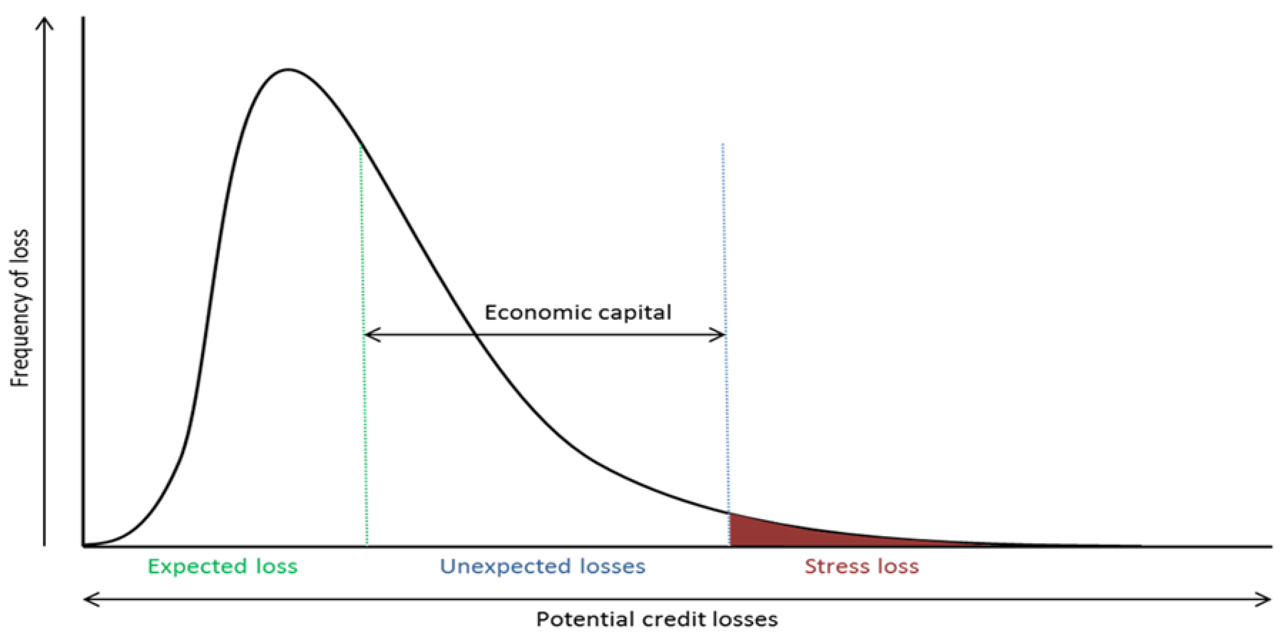
Mechanisms for allocating economic capital against credit risk, i.e., estimating the economic capital needed to support the credit risk activities, typically assume that the shape of the probability density function can be approximated by a distribution parametrized by the mean and standard deviation of the portfolio losses.

Figure 1 shows the Expected Loss (EL), which is the amount of credit loss that the bank expects on its credit portfolio in a given time horizon, i.e., the normal cost of businesses covered by provisioning and pricing policies, and the Unexpected Loss (UL), which is the portfolio risk. The standard deviation shows the average deviation of the expected losses. The likelihood that losses exceed the sum of EL and UL, i.e., the likelihood that the bank cannot meet its credit obligations by profits and capital, is given by the shaded area on the right-hand side of the curve, and it is usually indicated as the “stress loss”. The Value-at-Risk (VaR) is obtained as 100% minus the likelihood of the occurrence of stress loss at this confidence level. If the capital is determined in accordance with the gap between the EL and VaR, and if EL is covered by provisions or revenue, the likelihood that the bank will be solvent over an horizon of one-year is given by the confidence level.

The main concerns of regulators is the tail of the loss distribution which is strictly related to the value that the banks would set as a boundary for unexpected and stress loss. The total UL is not computed by aggregating individual ULs but depends on loss correlations between all loans belonging to the portfolio. The UL, or the portfolio’s standard deviation of credit losses, can be viewed as the sum of the contributions given by each of the individual credit facilities:

$$UL=\sum _{i=1}^N{\sigma }_i{\rho }_i$$

(1)

where ${\sigma }_i$ is the standard deviation of the credit losses for the ith facility, and ${\rho }_i$ represents the correlation between credit losses on the ith facility and those on the overall portfolio. The value ${\rho }_i$ is a parameter that represents the ith facility’s correlation/diversification effects with other instruments in the credit portfolio of the bank. Higher correlations among credit instruments, i.e., higher ${\rho }_i$, give a higher standard deviation of credit losses for the whole portfolio [12]. Basel II specifies the asset correlation for different asset classes by estimating asset correlations by a positive function of firm size and a negative function of firm default probability after adjustment for the obligor type over a time horizon of one year. It has been shown that differences in calculating the risk weights are mainly due to differences in IRB formulation models rather than differences in the risk of the portfolios being assessed. A reliable way of estimating risk is based on the calculation of joint loss distribution using the Vasicek model [14]. In the IRB framework of Basel II, the default probability (PD) per rating grade is the averaged percentage of obligors that will default over a one-year period. In the following text, we introduce the Vasicek model.

2.2. Systemic and Idiosyncratic Risk in the Vasicek Loan Portfolio Value Model

Regulations state that each financial institution needs to evaluate the probability distribution of the portfolio loss to estimate the necessary capital to support a portfolio of debt security. The equity capital allocated to the portfolio should assume the same percentile value of the distribution of the portfolio loss, corresponding to the probability stated by the rating level. The credit quality of the bank is related to the probability that the portfolio loss exceeds the equity capital. To determine the probability distribution of portfolio losses, one has to assume a model. In the following text, we introduce the Vasicek model [15], which allows, under certain assumptions, the distribution of the portfolio loss to be derived. The derived distribution converges to an analytical form as the portfolio size increases.

The Vasicek model is based on the assumption that the asset value of a given obligor is obtained by combining the effects of a systemic factor and an idiosyncratic one. Liabilities are modeled by adopting the hypothesis of a geometric Brownian motion driven by two continuous factors. The value $A_i$ of the i-th borrower’s assets is described by a stochastic differential equation (defining a standard geometric Brownian motion) and is determined by an aggregated level factor affecting all the i-th borrower’s assets and n statistically independent idiosyncratic factors:

$$d{A}_i={\mu }_i{A}_{i}dt+{\sigma }_i{A}_{i}d{X}_i$$

(2)

where ${\mu }_i$ is the drift rate, ${\sigma }_i$ the volatility of the value, and $x_i$ can be either the Wiener process or a Brownian motion, i.e., a continuous time random walk where the variation over any given time period has a normal distribution with zero mean and variance equal to the period length. Changes in separate time periods are also independent. It is worth noting that Equation (2) can be used to simulate the future prices of an asset, where ${\mu }_i$ is the mean of the asset return and ${\sigma }_i$ its standard deviation. At time T, one has the following asset value:

$$log{A}_i\left(T\right)=log{A}_i\left(0\right)+{\mu }_{i}T-\frac{1}{2}{\sigma }_i^{2}T+{\sigma }_i\sqrt{T}{X}_i$$

(3)

with $X_i\sim N(0,1)$.

It is straightforward to write Equation (3) as

$$A_i\left(T\right)=A_i\left(0\right)e^{({\mu }_i-\frac{1}{2}{\sigma }_i^2)T+{\sigma }_i\sqrt{T}{X}_i}.$$

(4)

The default of the i-th loan occurs if $A_i\left(T\right)<B_i$, with $B_i$ being a fixed value. One can evaluate the probability of such an event as

$$P[X_i<c_i]=N\left(c_i\right)=p^{*}$$

(5)

where $c_i$ is easily derived by Equation (4) when one sets the default threshold as $B_i$, i.e., $c_i=\frac{log{B}_i-log{A}_i-{\mu }_{i}T+\frac{1}{2}{\sigma }_i^{2}T}{{\sigma }_i\sqrt{T}}$; N is the cumulative normal distribution function. Then, a single obligor default happens if the value of a normal random variable goes below $c_i$.

The correlation among defaults is introduced by assuming correlation in the $A_i$ processes and then in the terminal values $A_i\left(T\right)$. In detail, $X_{i}s$ in (4) is assumed to be pair-wise correlated according to the factor $\rho$. The main assumption of the model is that because each random variable $X_i$ is normal and equi-correlated, it can be computed as the sum of two other random variables such that one is common across firms and the other is idiosyncratic.

$$X_i=z\sqrt{\rho }+{ϵ}_i\sqrt{1-\rho }$$

(6)

with $z\sim N(0,1)$ (standard normal distribution) and the same ${ϵ}_i\sim N(0,1)$. Then, it is straightforward to get

$$P[X_i<c_i]=N\left(\frac{N^{-1}\left(p^{*}\right)-z\sqrt{\rho }}{\sqrt{1-\rho }}\right).$$

The proportion of loans in a portfolio that suffers default is given by the following cumulative distribution function:

$$Pr[p\left(z\right)\le x]=P[z\ge p^{-1}\left(x\right)]=N(-p^{-1}\left(x\right))=N\left(\frac{\sqrt{1-\rho }{N}^{-1}\left(x\right)-N^{-1}\left(p\right)}{\sqrt{\rho }}\right),$$

and this depends on p and $\rho$ for each portfolio.

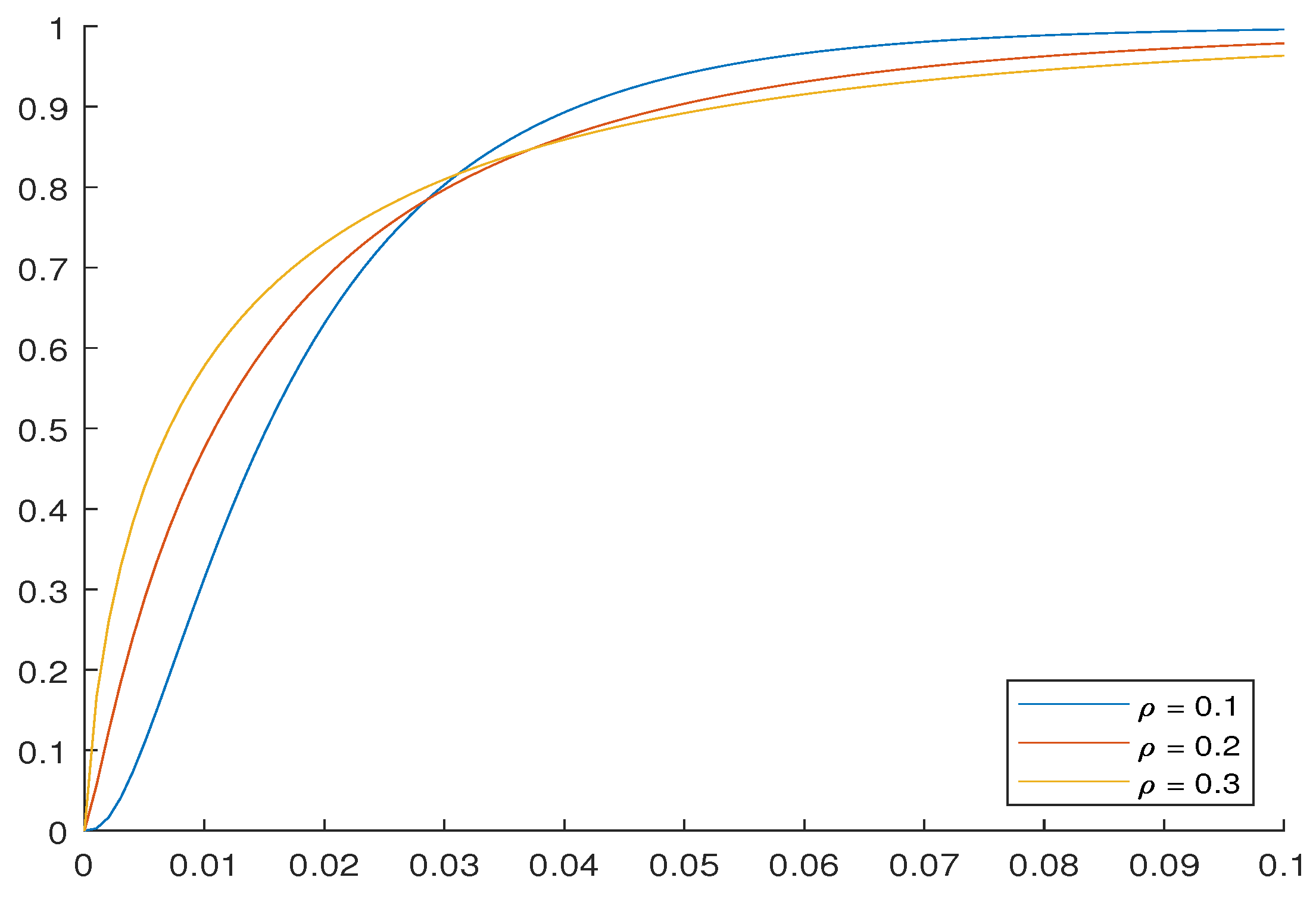
Then, we observe that in the context of the Vasicek model, a simple threshold condition determines whether the obligor defaults or not. This is interpreted in the context of a trigger mechanism, which is useful for modeling credit risk. The cumulative distribution function of the proportion of losses that suffers default is defined by two parameters, i.e., the default probability p and the asset correlation $\rho$. In Figure 2, we show different unconditional cumulative default probabilities obtained for $p=0.02$ and different values of $\rho$.

2.3. Dynamics of Credit Risk Contagion

Contagion, or “frailty”, is represented by unobservable explanatory variables that are correlated across firms and represent non-performing loans. There are many open questions in the scientific literature on credit risk contagion. A very important one investigates why corporations fail to fulfill all obligations at the same time, giving different explanations. Firms may present common or correlated risks factors, whose interactions cause correlated changes in the probability of default. Secondly, a default may be contagious, so that one event in a corporation may cause the failure of another one [16]: Models should account for the degree of time clustering in defaults that are observed in the data. In [16], the authors found evidence from time data of default clustering beyond that predicted by the standard doubly stochastic model of default for US corporations over the period from 1979 to 2004. It is evident that if defaults are highly clustered, more than that depicted by standard models, banks need to consider greater capital to survive default losses (especially when high confidence levels, such as 99.9%, are required). Collin-Dufresne et al. [17] suggests, based on experimental findings that default induces increases in the conditional default probabilities of other firms, while Kusuoka [18] puts it in relation to the default risk premia of other firms. “For example, the collapses of Enron and WorldCom could have caused a sudden reduction in the perceived precision of accounting leverage measures of other firms. Indeed, in [19] empirical evidence is found that all other things equal, a reduction in the measured precision of accounting variables is associated with a widening of credit spread. Lang and Stulz (1992) [20] explored evidence of default contagion in equity prices.”

3. Credit Risk Contagion on Networks

Linkages among financial institutions appear to greatly influence the dynamics of the spreading of credit risk; moreover, interconnectedness seems to crucially affect stability. The theory of networks seems to be the more appropriate language to characterize linkages and their related dynamics. Financial networks [21] help to understand how externalities move along financially related structures and may build up to systemic risk, especially when incomplete information and incomplete risk markets have to be considered [22].

Originally, the connection topology has been assumed to be regular or completely random ([23]). Many real-world networks, however, can be considered to be living in between these two extremes. Small-world networks are regular networks “rewired” to introduce increasing amounts of disorder. These networks can be highly clustered, like regular lattices, with small characteristic path lengths, like random graphs [24]. Another important branch of this field regards the optimization of connectivity of financial systems [25]. We do not address this issue in the present paper, but we plan to address this issue within the context of the proposed model in our future research.

A network of N nodes and L links is fully characterized by its binary or weighted adjacency matrix $A=\left[a_{ij}\right],1\le i,j\le N$. The binary matrix is such that the entry $a_{ij}$ is simply 1 or 0 depending on whether the $ith$ and $jth$ nodes are connected or not. For a weighted matrix, each entry $w_{ij}$ is equal to the weight of the link between i and j. In the case of a directed graph, the links are oriented from node i to node j, so that $w_{ij}\ne w_{ji}$. For undirected graphs, the adjacency matrix is symmetric.

In our model, each node is a financial institution represented by a portfolio of risky assets, and the linkages among nodes are due to financial relations by means of credit swaps between the two linked institutions. We model the network as an undirected binary graph to focus on the basic influence of the architecture of the network on the contagion dynamics.

Real-world networks are usually very different from regular lattices. They are mostly heterogeneous and exhibit dynamic self-organization phenomena, typical of complex systems. The patterns defined by the connectivity properties of real-world networks strongly affect the evolution of epidemic, reactive-diffusive processes of contagion. The statistical distributions related to the features of real-world networks are often heavy-tailed, and this property is very important with respect to risk.

We define the risk of a financial institution by applying the Vasicek model and introducing a random variable for the i-th bank as

$$y_i=-{\mathsf{\Phi }}^{-1}\left(p_i\right)+z\sqrt{{\rho }_i}+{ϵ}_i\sqrt{1-{\rho }_i}$$

(7)

with $\mathsf{\Phi }(·)$ cdf being a standard normal random variable. z is the systemic risk factor, and ${ϵ}_i$ are the idiosyncratic ones; they are both standard normal random variables. Finally, ${\rho }_i$ is the risk correlation between two different banks, and $p_i$ is the probability of failure of the i-th bank [8]. Failure happens when $y_i<0$. One can easily derive (see [8])

$$Pr(y_i<0)=p_i.$$

(8)

From Equation (7), it is clear that for ${\rho }_i=0$, there is no systemic risk and failures are statistically independent. On the contrary, when ${\rho }_i=1$, we only have systemic risk, and failures are perfectly correlated. In choosing ${\rho }_i$ one can follow Basel II [12] by setting

$${\rho }_i=0.12\frac{1-e^{-50P{D}_i}}{1-e^{-50P}}+0.24\left(1-\frac{1-e^{-50P{D}_i}}{1-e^{-50}}\right)\sim 0.12\left(1+e^{-50P{D}_i}\right)$$

(9)

with $P{D}_i$ being the probability of default of firm i over one year, ignoring credit contagion effects. Quantities $p_i$ are predicted from tables provided by rating agencies.

Spreading of Systemic Risk Using the SIIS (Susceptible-Infected1-Infected2-Susceptible) Model

The epidemic modeling metaphor has been widely used to describe a large range of different phenomena which can be conceptually thought of as contagion processes [26]. That is why epidemic models are widely diffused and represent a cornerstone that crosses different disciplines. Moreover, their efficiency has been improved in recent years due to the integration of large-scale datasets. Epidemic models are constructed to describe the evolution of the contagion process within a population. In our paper, the population is structured into a network architecture, inserting into the wide stream of scientific literature unfolding dynamical processes in complex networks [3].

The assessment of credit risk in large banks has changed consistently in the last few years. It used to be common to manage the origination process (evaluation of whether a new business should be accepted or rejected), but now it can be managed by using credit derivatives and securitization with loans and bonds as collateral assets (CLOs, collateralized loan obligations; CBOs collateralized bond obligations; CDOs collateralized debt obligations).

This phenomenon, while it may limit the idiosyncratic risk, can be a source of systemic risk; in our model, it is represented by assuming the possibility of a transition from assets infected by idiosyncratic risk to those infected by systemic risk.

The agents of our model are risky assets belonging, for each node, to a bank’s portfolio. Contagion occurs through infection by non-performing loans.

We approach the mathematical representation of credit risk spreading in an interbank network by adopting the simplest definition of epidemic dynamics, which considers the population as fixed, ignoring migration both among the nodes and among birth or death processes. Compartmentalization is a derivation of the simplest two-state susceptible-infected-susceptible (SIS) model, a cornerstone in epidemic spreading modelization and, on the other hand, a widely used modeling scheme for knowledge and information diffusion within social systems. It is worth mentioning here that the heterogeneity of agents is an important issue in this research field, one addressed by the authors in [27]. Very interesting multi-scale approaches have also proposed by different papers by S. Havlin (see, for instance [28]). However, it is not the scope of the present paper to include this effect in the model, as we mostly intend to focus on the effect of the network structure on the epidemic spreading of non-performing loans.

The classical approach divides the population into two classes: susceptibles (who can contract the disease) and infectious (who have contracted the infection and can be contagious). Then, one has to define the process governing the transition of agents from one class to another in order to describe the dynamic evolution of the process of contagion within the population. The classical SIS does not assume the possibility of becoming immune, thus undergoing a cycle of $S\to I\to S$.

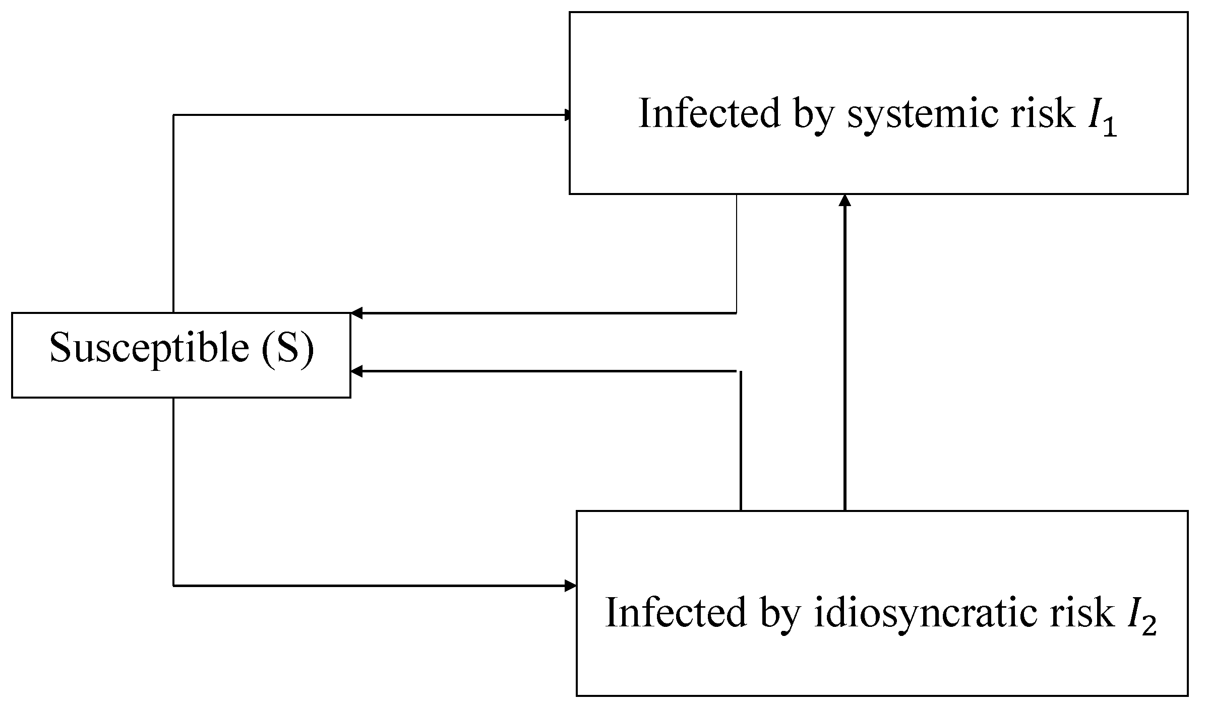
In our model, we extend the classical approach by dividing the population for each node into three classes: susceptibles S, i.e., those that may be infected by credit risk, infectious1 (default fraction due to systemic risk) $I_1$, and infectious2 (default fraction due to idiosyncratic risk) $I_2$. Idiosyncratic risk can be considered to be endemic to a particular asset, depending, for instance, on fluctuations in the stock market or in the interest rates, and then it can be mitigated by diversification. Figure 3 illustrates the transfer diagram for the SIIS model [29] adopted here.

Both infected assets may recover to the susceptible state.

We define the process governing the transition of credits from one class to another when the population is structured into a network with the following system of ODEs (Ordinary Differential Equations):

$$\left\{\begin{array}{cc}{\dot{S}}_i\left(t\right)\hfill & =-S_i\left(t\right){\rho }_i{I}_{2i}\left(t\right)-S_i\left(t\right)\sum _{j=1}^N{a}_{ij}{I}_{1j}+\psi (I_{1i}\left(t\right)+I_{2i}\left(t\right))\hfill \\ {\dot{I}}_{1i}\left(t\right)\hfill & =S_i\left(t\right)\sum _{j=1}^N{a}_{ij}{I}_{1j}\left(t\right)-\psi I_{1i}\left(t\right)+r{I}_{1i}\left(t\right)I_{2i}\left(t\right)\hfill \\ {\dot{I}}_{2i}\left(t\right)\hfill & =S_i\left(t\right){\rho }_i{I}_{2i}\left(t\right)-\psi I_{2i}\left(t\right)-r{I}_{1i}\left(t\right)I_{2i}\left(t\right)\hfill \end{array}\right.$$

(10)

where $S_i\left(t\right)$, $I_{1i}\left(t\right)$, and $I_{2i}\left(t\right)$ represent the populations of each compartment within node i at time t, $\psi$ is the recovery rate, and r is the contagion rate. The adjacency matrix $A=\left[a_{ij}\right],1\le i,j\le N$ characterizes interrelations among the N institutions, and its form determines the structure of the financial network.

4. Numerical Experiments

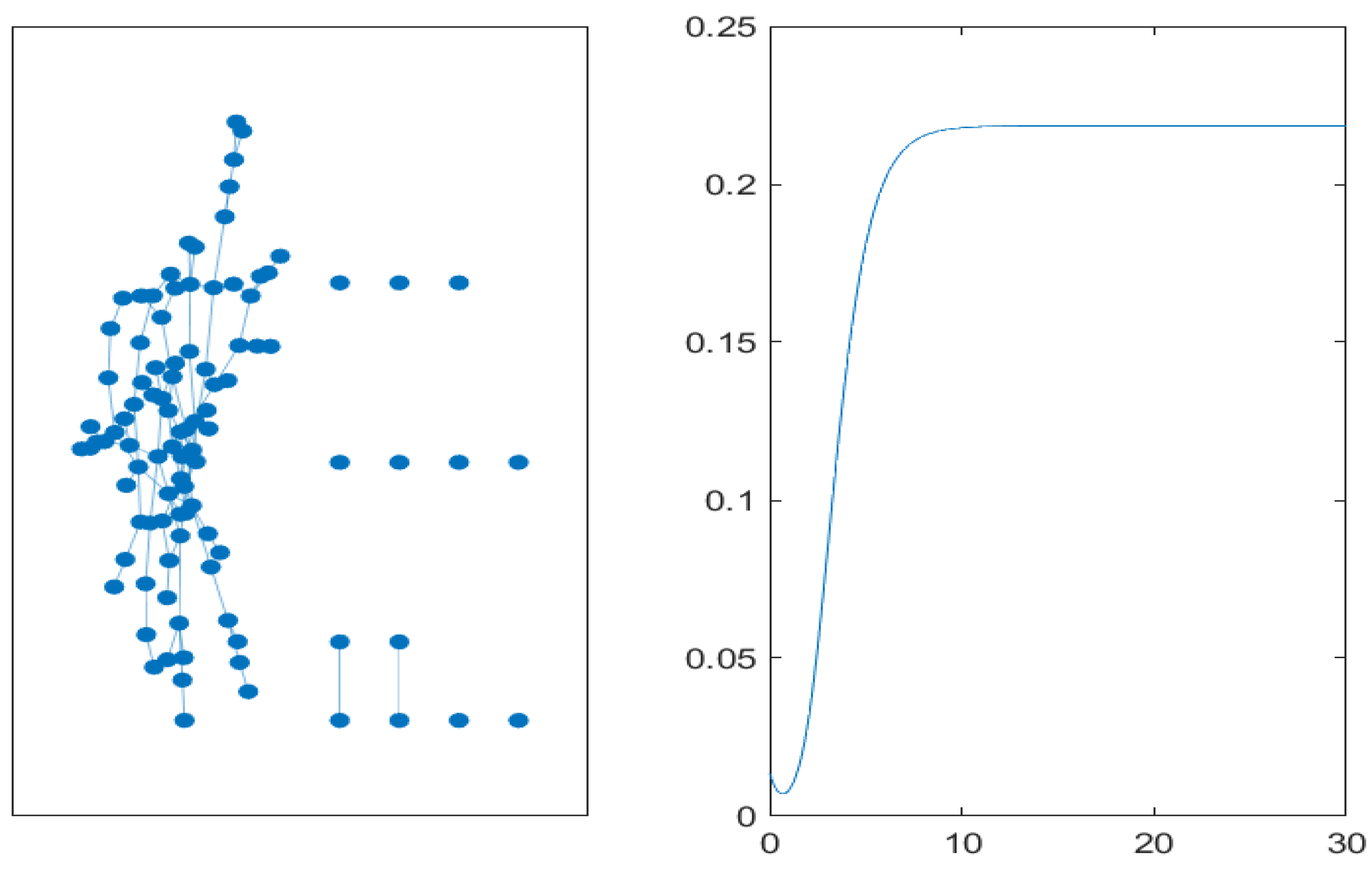
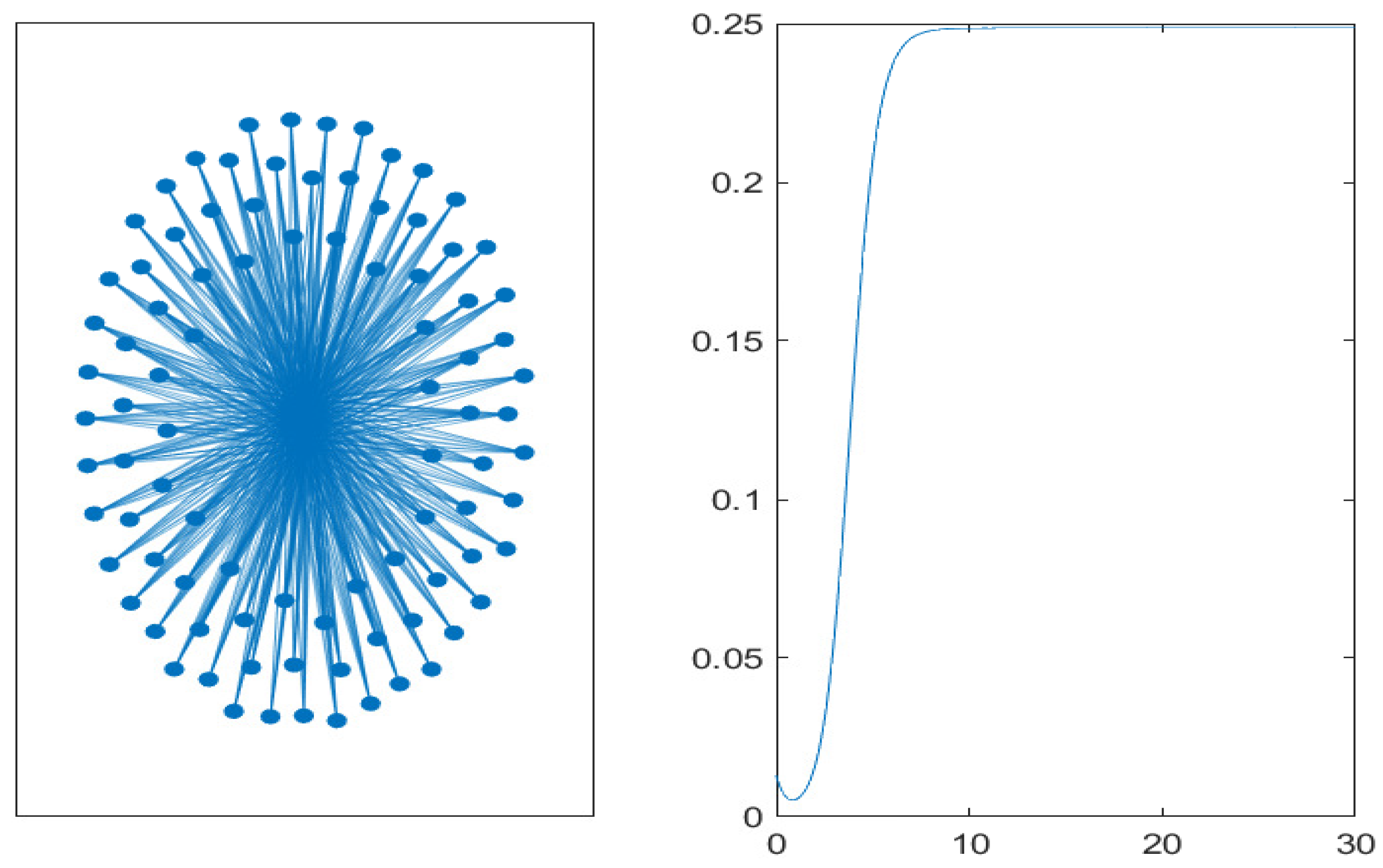
In this section, we perform some numerical experiments with the aim of analyzing the dynamics of systemic risk on different topological structures of networks. We adopt the epidemic model splitting agents affected by idiosyncratic risk from those affected by systemic risk, as previously introduced. We aim to compare the effect of credit risk contagion on two different network structures: the basic model for random graphs, i.e., the Erdös–Rényi for different significant connection probabilities, the core-periphery network for different levels of balance between core nodes and periphery nodes [11], and the small-world networks (Watts–Strogatz networks) for increasing rewiring probability values. In our numerical experiments, we consider a network with 100 nodes in all simulations (it is worth noting that the number of nodes does not influence the results), each of them characterized by a given portfolio with random numbers of assets and correlations. Then, we evaluate the 5% VaR (Value at Risk) of the assets as infectious. The time evolution of the epidemic process is then determined by the system of Equation (10), and during the time evolution, we analyze the mean value of assets subject to systemic risk when different topological structures of the underlying network are assumed. We use the fixed recovery rate ($\psi =2$) and contagion rate ($r=0.1$) to emphasize the effect of the network structure on the dynamics. We use an exponential distribution to characterize the initial distribution of assets affected by systemic risk on each node, and we evaluate the credit risk at the 5% level by calculating the related percentile. Given this setting, we run three different simulations of the dynamics of contagion on the random network structure on the core-periphery structure and on the small-world network, in each case assuming the model of contagion (10). The basic parameters of the model of epidemic spreading, i.e., the recovery rate and the contagion rate, are the same for all network structures for the sake of a better comparison.

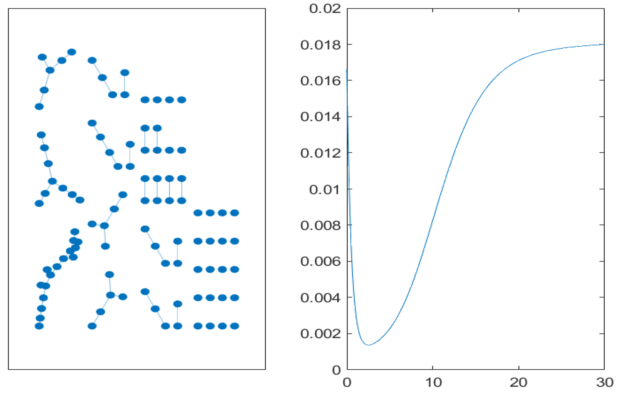
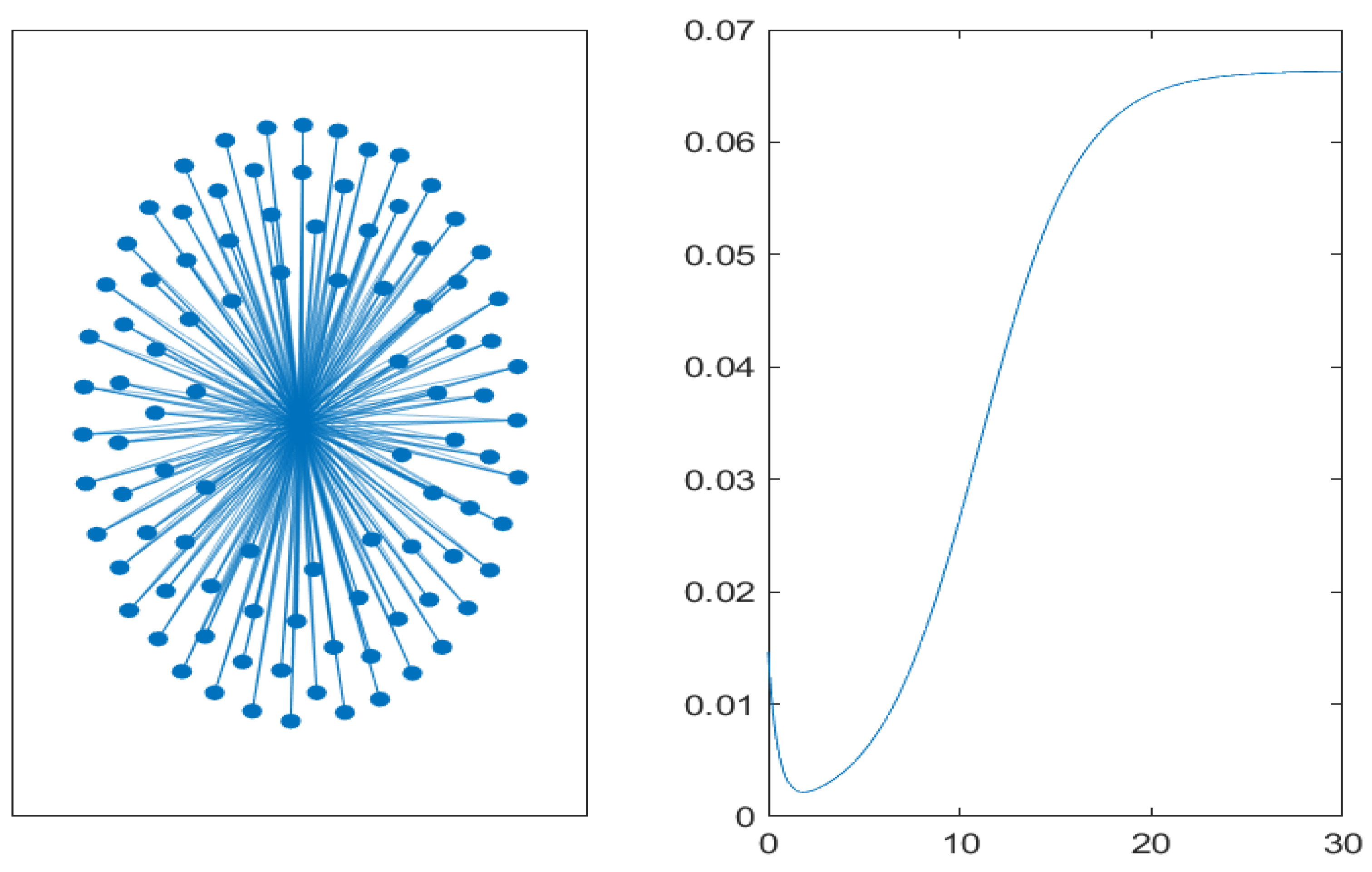
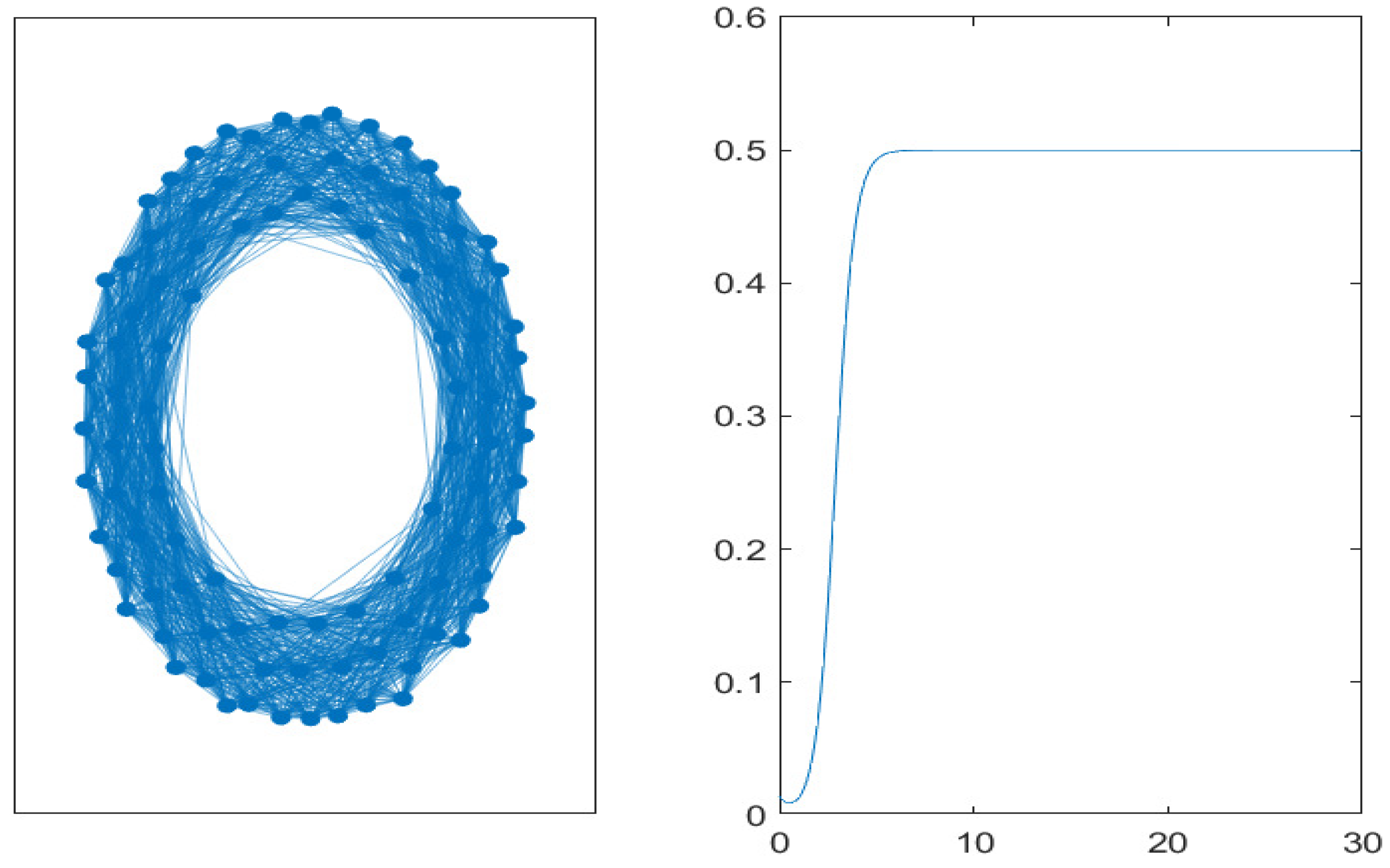
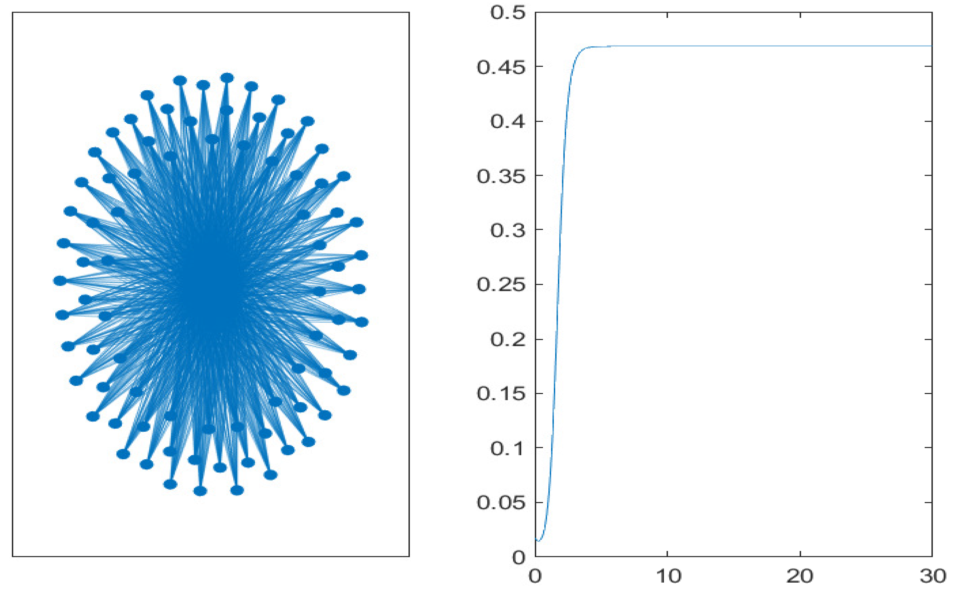
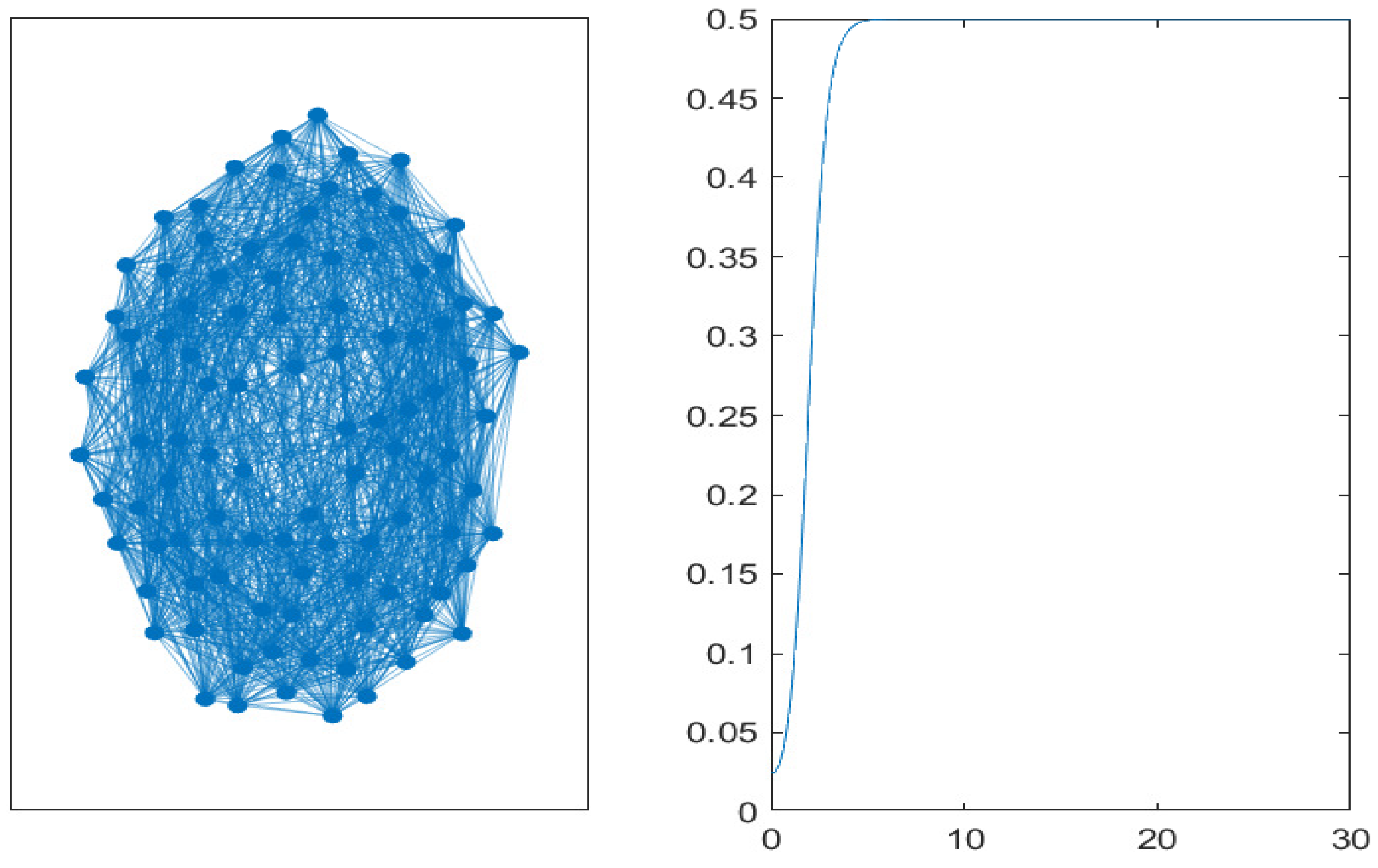
Each simulation adopts different connection probabilities for the Erdös–Rényi network, which represent typical threshold values. The first value ($p=0.01$) is related to the appearance of the first linkages, the second ($p\sim 0.02$) is the value related to the existence of a giant component, and the third one ($p=0.4$) provides a connected network, with a few nodes representing exceptions. For each simulation, we evaluate the dynamics of the mean value of assets subject to systemic risk on the network whose graphical representation is provided on the right-hand side of each figure (codes available upon request to the authors). In Figure 4, we use a realization of an Erdös–Rényi random graph with a connection probability of $p=0.01$ (represented on the left) to simulate the SIIS model given by Equation (10). In the right part of the figure, we report the time evolution of the mean of the subset of the population infected by systemic risk (non-performing loans). After a transient, a steady-state value of about 1.8% is attained for the whole population. The value appears quite low in accordance with the low level of network connectivity. In Figure 5, an analogous simulation on a core-periphery network is performed. We use five core nodes over the total number of nodes corresponding to a low connectivity level as well. Although the steady-state value is higher, a similar transient with respect to the low-connectivity random network is observed. To end this first part of the simulations, i.e., with low connectivity, we run the model on a small-world network by increasing the rewiring probability to $beta=0.1$ (ring network); results are shown in Figure 6. In this case, both the rate of increase and the mean values of the non-performing loans are much higher than in the previous network structures. Simulations with higher connectivity values are reported in Figure 7 and Figure 8 for the random and core-periphery networks, respectively. It is interesting to observe that in this case, similar transients can be observed, even with different steady-state values. Also, the increased connectivity leads to closer steady-state values in the two network representations. In Figure 9, we run the model on a small-world network with a slightly higher rewiring probability of $beta=0.1$. Also, in this case, both the rate of increase and the mean values of non-performing loans are much higher than in the previous network structures.

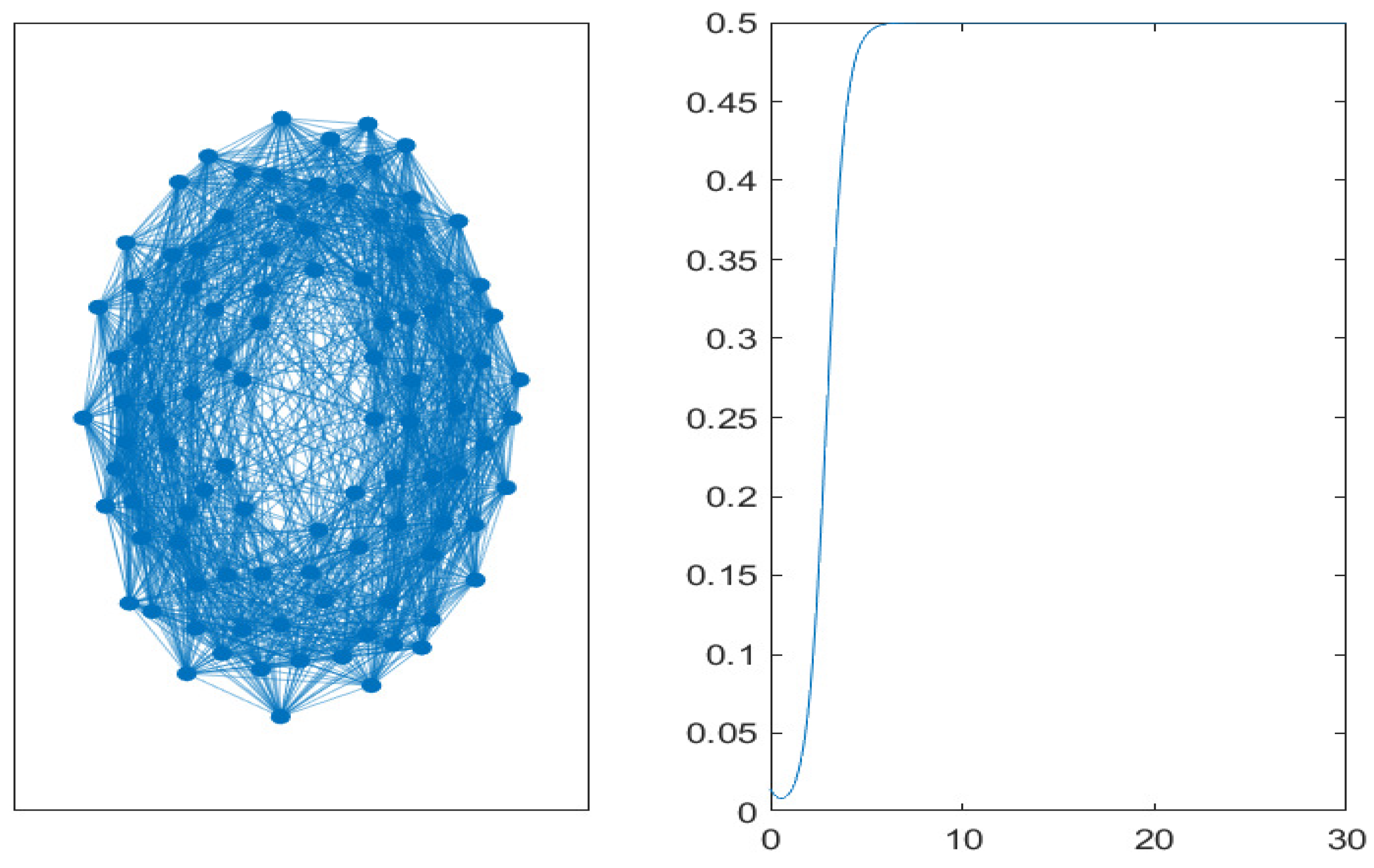
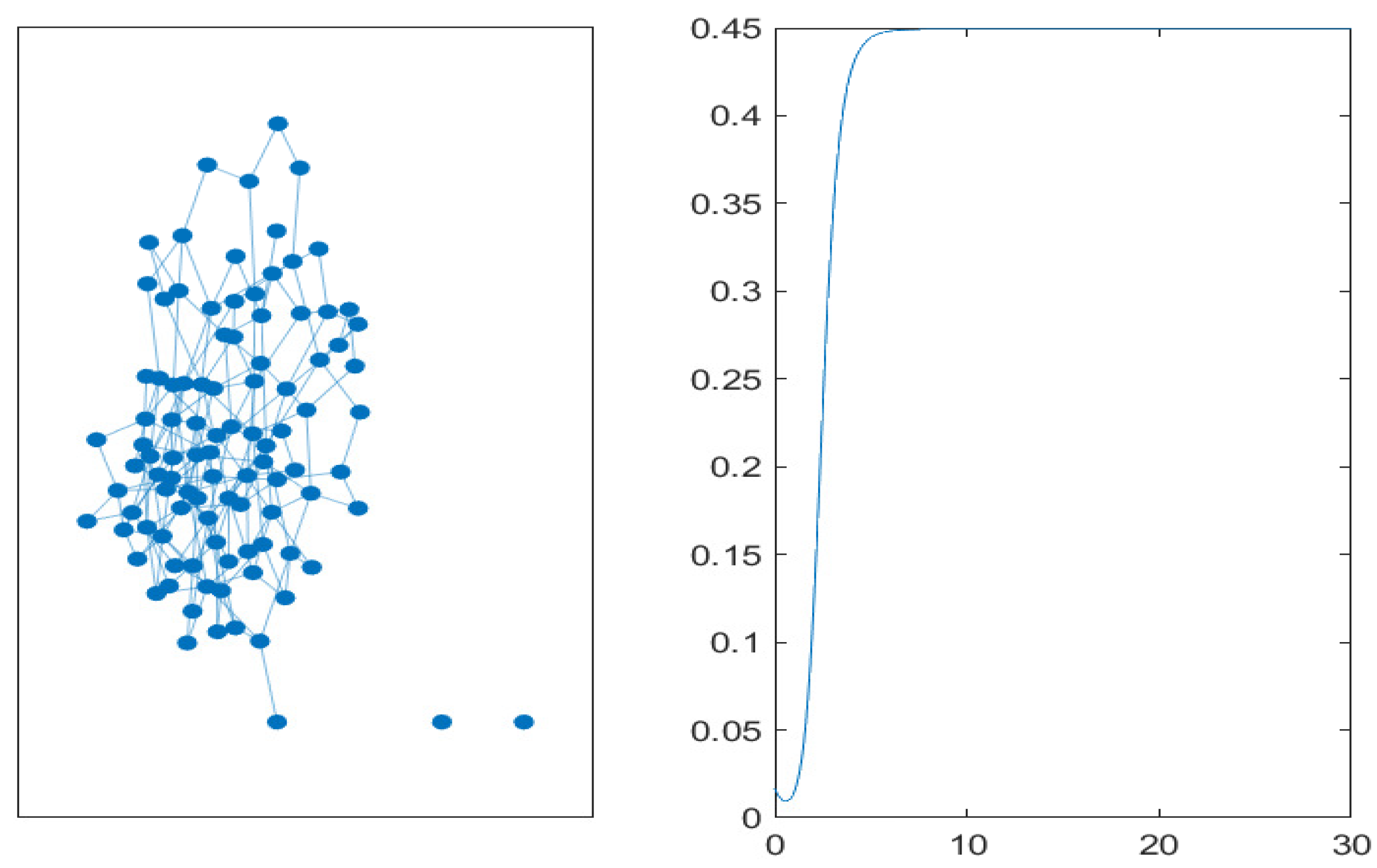
Finally, in Figure 10, Figure 11 and Figure 12, networks with high connectivity are simulated. Again, the duration of the transient phase is quite similar in the two representations, and the steady-state values are closer. In the small-world network with a rewiring probability of $\beta =0.2$, the steady-state value of non-performing loans is similar to the previous simulations, but the rate of increase is even higher.

In summary, from the point of view of the epidemic spreading of systemic risk, the random graph, usually considered to be a “benchmark ”network topology structure, can be considered to be being almost equivalent to the core-periphery topological structure, in the case in which the probability of linkages in the random network is related to the ratio between the core and the peripheral nodes. Specifically, by increasing the probability of linkages in the random network, the effects on the long-term solutions are analogous, both in terms of the time interval needed for stabilization and in terms of the average long-term value for the systemic risk-infected assets based on the results obtained by increasing the number of core nodes in the core-periphery structure. The small-world network has a quite different behavior characterized by a higher positive rate of infectious spreading by non-performing loans in the structure.

5. Conclusions and Research Perspectives

When assessing the risk of credit portfolios as well as investment portfolios, banks should look not only at the risk of individual exposures but also at possible exposure correlations. There have been different attempts to measure risk at the level of the banking system [30]. Our paper enters this stream of research by adopting a model of risk contagion which distinguishes between systemic and idiosyncratic risk. Usually, the probability of systemic risk is thought of in terms of the fraction of financial institutions whose portfolios are affected by systemic risk. We numerically explored the long-term solutions of a model of epidemic credit risk spreading on networks for two different topological structures with different levels of connectivity. Our numerical results show that connectivity increases the spreading of assets infected by systemic risk in the network, in the case of random graphs. In the case of a core-periphery structure, the spreading is controlled by diminishing the number of core institutions. The numerical experiments show that the spread of credit risk is analogous in network structures of the Erdös–Renyi random type and core-periphery type when the probability of linkages in the first type is compared to the ratio of core nodes and periphery nodes. It is worth noting that the quality and specific category of credit risk should be defined; we did not address this issue in the present paper, as our model focuses on the network properties. Our research plans are to extend the model by providing specifications regarding the risk categories. Of course, specifying risk implies the use of directed networks, i.e., one can use the same network structure but with unilateral links with the direction determined by the quality of the risk. Moreover, heterogeneity in size (see the seminal review [31,32], not only in centrality, might be worth analyzing using a future extension of the proposed model.

One research perspective would be to analyze the propagation of asymmetric information, i.e., the consequences of information imperfections propagating through the structure, and how this propagation may affect the network’s performance in terms of resilience. Resilience is defined in many different ways; one definition is the ability of structures, which have been impacted by external shocks, to recover and adapt to new conditions. In any case, thinking about resilience requires the assessment of potential future threats at the scale of systems, rather than at the scale of individual components. As proposed by Helbing [33], a useful approach for influencing complex systems, is to support the self-organization and self-control of the system, rather than adopting controlling actions in the conventional way. This approach would lead to a more flexible and adaptive system that is more able to cope with challenges coming from external perturbations. One may benefit from some basic characteristics of complex systems which through self-organization, can be adapted to the environment and are often robust and resource-efficient. For instance, decentralized coordination strategies, which have already been successfully applied in traffic control, may be more efficient than centralized ones. There is also the possibility of decompartmentalization of a network into weakly coupled, or even uncoupled, sub-networks. Data could be retrieved from the literature. For instance, an interesting source is provided in [34], where authors construct a matrix of interbank loans for Switzerland based on known marginal loan distributions. Simulated experiments, analyses of real-world financial data, and theoretical insights may improve regulations, increasing financial stability.

References

1. Jackson, M.O. Social and Economic Networks; Princeton University Press: Pinceton, NJ, USA, 2008. [Google Scholar]
2. Vega-Redondo, F. Complex Social Networks; Econometric Society Monographs; Cambridge University Press: Cambridge, UK, 2007. [Google Scholar]
3. Pastor-Satorras, R.; Castellano, C.; Van Mieghem, P.; Vespignani, A. Epidemic processes in complex networks. Rev. Mod. Phys. 2015, 87, 925–979. [Google Scholar] [CrossRef] [Green Version]
4. Batiz-Zuk, E.; López-Gallo, F.; Martínez-Jaramillo, S.; Solórzano-Margain, J.P. Calibrating limits for large interbank exposures from a system-wide perspective. J. Financ. Stabil. 2016, 27, 198–216. [Google Scholar] [CrossRef]
5. BCBS. Macroeconomic Impact Assessment of OTC Derivatives Regulatory Reforms; Assessment Group on Derivatives Report Base Committee for Banking Supervision—Bank for International Settlements. 2013. Available online: https://www.bis.org/publ/othp20.pdf (accessed on 9 June 2019).
6. Amini, H.; Cont, R.; Minca, A. Stress testing the resilience of financial networks. Int. J. Theor. Appl. Financ. 2012, 15, 1250006. [Google Scholar] [CrossRef]
7. Battiston, S.; Martinez-Jaramillo, S. Financial networks and stress testing: Challenges and new research avenues for systemic risk analysis and financial stability implications. J. Financ. Stabil. 2018, 35, 6–16. [Google Scholar] [CrossRef]
8. Martinez-Miera, D.; Repullo, R. Does competition reduce the risk of bank failure? Rev. Financ. Stud. 2010, 23, 3638–3664. [Google Scholar] [CrossRef]
9. León, C.; Machado, C.; Sarmiento, M. Identifying central bank liquidity super-spreaders in interbank funds. J. Financ. Stabil. 2018, 35, 75–92. [Google Scholar] [CrossRef]
10. Dastkhan, H.; Garneh, N.S. How the ownership structures cause epidemics in financial markets: A network-based simulation model. Phys. A 2018, 492, 324–342. [Google Scholar] [CrossRef]
11. Frey, R.; Hledik, J. Diversification and Systemic Risk: A Financial Network Perspective. Risks 2018, 6, 54. [Google Scholar] [CrossRef]
12. Basel Committee on Banking Supervision 2005. International Convergence of Capital Measurement and Capital Standards, a Reviewed Framework. Available online: https://www.bis.org/publ/bcbs128.htm (accessed on 9 June 2019).
13. Basel III: A Global Regulatory Framework for More Resilient Banks and Banking Systems. Banking for International Settlements. 2010. Available online: https://www.bis.org/publ/bcbs189.htm (accessed on 9 June 2019).
14. Chatterjee, S. Modelling Credit Risk; Centre for Central Banking Studies, Bank of England: London, UK, 2015. [Google Scholar]
15. Vasicek, O. The Distribution of Loan Portfolio Value. Risk 2002, 15, 160–162. [Google Scholar]
16. Das, S.R.; Kapadia, N.; Saita, L. Common failings: How corporate defaults are correlated. J. Financ. 2007, 62, 93–118. [Google Scholar] [CrossRef]
17. Collin-Dufresne, P.; Goldstein, R.S.; Martin, J.S. The Determinants of Credit Spread Changes. J. Financ. 2001, 56, 2177–2207. [Google Scholar] [CrossRef]
18. Kusuoka, S. A Remark on default risk models. In Advances in Mathematical Economics; Springer: Tokyo, Japan, 1999; pp. 69–82. [Google Scholar]
19. Yu, F. Accounting Transparency and the Term Structure of Credit Spreads. Swiss J. Econ. Stat. 2005, 75, 53–84. [Google Scholar] [CrossRef]
20. Lang, L.H.P.; Stulz, R.M. Contagion and competitive intra-industry effects of bankruptcy announcements: An empirical analysis. J. Financ. Econom. 1992, 32, 45–60. [Google Scholar] [CrossRef]
21. Haldane, A. Rethinking the Financial Network. Speech by Mr Andrew Haldane, Executive Director, Financial Stability, Bank of England at the Financial Student Association, Amsterdam. 28 April 2009. Available online: https://www.bis.org/review/r090505e.pdf (accessed on 10 February 2019).
22. Stiglitz, J.E. The contributions of the economics of information to twentieth century economics. Q. J. Econ. 2000, 115, 1441–1478. [Google Scholar] [CrossRef]
23. Solomonoff, R.; Rapoport, A. Connectivity of random nets. Bull. Math. Biophys. 1951, 13, 107–117. [Google Scholar] [CrossRef]
24. Bollobás, B. Random Graphs, 2nd ed.; Cambridge University Press: Cambridge, UK, 2001. [Google Scholar]
25. Martinez-Jaramillo, S.; Carmona, C.U.; Kenett, D.Y. Interconnectedness and financial stability. J. Risk Manag. Financ. Inst. 2019, 12, 168–183. [Google Scholar]
26. Garas, A.; Argyrakis, P.; Rozenblat, C.; Tomassini, M.; Havlin, S. Worldwide spreading of economic crisis. New J. Phys. 2010, 12, 113043. [Google Scholar] [CrossRef]
27. Dolfin, M.; Leonida, L.; Outada, N. Modeling human behavior in economics and social science. Phys. Life Rev. 2017, 22–23, 1–21. [Google Scholar] [CrossRef]
28. Gontis, V.; Havlin, S.; Kononovicius, A.; Podobnik, B.; Stanley, H.E. Stochastic model of financial markets reproducing scaling and memory in volatility return intervals. Phys. A 2016, 462, 1091–1102. [Google Scholar] [CrossRef] [Green Version]
29. Knopoff, D.; Trucco, F.A. A compartmental model for antibiotic resistant bacterial infections over networks. Int. J. Biomath. in press.
30. Lehar, A. Measuring Systemic Risk: A Risk Management Approach. J. Bank. Financ. 2005, 29, 2577–2603. [Google Scholar] [CrossRef]
31. Babus, A.; Allen, F. Networks in finance. In Network-Based Strategies and Competencies; Kleindorfer, P., Wind, J., Eds.; Wharton School Publishing: Upper Saddle River, NJ, USA, 2009; pp. 367–382. [Google Scholar]
32. Glasserman, P.; Young, P. Contagion in financial networks. J. Econ. Lit. 2016, 54, 779–831. [Google Scholar] [CrossRef]
33. Helbing, D. Systemic Risks in Society and Economics. IRGC—Emerging Risks. October 2010. Available online: https://ssrn.com/abstract=2413205 (accessed on 9 June 2019).[Green Version]
34. Sheldon, G.; Maurer, M. Interbank lending and systemic risk: An empirical analysis for Switzerland. Swiss J. Econ. Stat. 1998, 134, 685–704. [Google Scholar]
Figure 1. Frequency of loss as a function of potential credit losses.
Mathematics 07 00713 g001
Figure 2. Unconditional cumulative probabilities of default for a default probability of p = 0.02 and different values of asset correlation ρ .
Mathematics 07 00713 g002
Figure 3. Transfer diagram for the S I I S (Susceptible-Infected1-Infected2-Susceptible) model. Boxes represent compartments, and arrows represent the transition from one compartment to another.
Mathematics 07 00713 g003
Figure 4. Low level of connectivity:Erdös–Rényi graph with 100 nodes and a connection probability of p = 0.01 (left). Time evolution of the mean value of non-performing loans on the graph (right).
Mathematics 07 00713 g004
Figure 5. Core-periphery graph with five core nodes and 95 periphery nodes (left). Time evolution of the mean value of non-performing loans on the graph (right).
Mathematics 07 00713 g005
Figure 6. Small-world (Watts-Strogatz) network with 100 nodes and a rewiring probability of β = 0 (ring) (left). Time evolution of the mean value of non-performing loans on the graph (right).
Mathematics 07 00713 g006
Figure 7. Medium level of connectivity:Erdös–Rényi graph with 100 nodes and a connection probability of p 0.02 (left). Time evolution of the mean value of non-performing loans on the graph (right).
Mathematics 07 00713 g007
Figure 8. Core-periphery graph with 10 core nodes and 90 periphery nodes (left). Time evolution of the mean value of non-performing loans on the graph (right).
Mathematics 07 00713 g008
Figure 9. Small-world (Watts-Strogatz) network with 100 nodes and a rewiring probability of β = 0.1 (left). Time evolution of the mean value of non-performing loans on the graph (right).
Mathematics 07 00713 g009
Figure 10. High level of connectivity: Erdös–Rényi graph with 100 nodes and a connection probability of p = 0.04 (left). Time evolution of the mean value of non-performing loans on the graph (right).
Mathematics 07 00713 g010
Figure 11. Core-periphery graph with 20 core nodes and 80 periphery nodes (left). Time evolution of the mean value of non-performing loans on the graph (right).
Mathematics 07 00713 g011
Figure 12. Small-world (Watts–Strogatz) network with 100 nodes and a rewiring probability of β = 0.2 (left). Time evolution of the mean value of non-performing loans on the graph (right).
Mathematics 07 00713 g012