On the Parametrization of Caputo-Type Fractional Differential Equations with Two-Point Nonlinear Boundary Conditions

Abstract

In this paper, we offer a new approach of investigation and approximation of solutions of Caputo-type fractional differential equations under nonlinear boundary conditions. By using an appropriate parametrization technique, the original problem with nonlinear boundary conditions is reduced to the equivalent parametrized boundary-value problem with linear restrictions. To study the transformed problem, we construct a numerical-analytic scheme which is successful in relation to different types of two-point and multipoint linear boundary and nonlinear boundary conditions. Moreover, we give sufficient conditions of the uniform convergence of the successive approximations. Also, it is indicated that these successive approximations uniformly converge to a parametrized limit function and state the relationship of this limit function and exact solution. Finally, an example is presented to illustrate the theory.

1. Introduction

In recent years, fractional differential equations subjected to different kind of boundary conditions have been studied such as periodic/anti-periodic, nonlocal, multipoint, and integral boundary conditions, see [1,2,3].

In this paper, we consider Caputo-type fractional differential equations with nonlinear boundary conditions. We apply the technique proposed in [4,5,6,7,8,9,10,11] for investigation and approximation of solutions of Caputo-type fractional differential equations with nonlinear boundary conditions. By using an appropriate parametrization technique, nonlinear boundary conditions are transformed to linear boundary conditions by using vector parameters. To study the transformed problem, we construct a numerical-analytic scheme which is successful in relation to different types of two-point and multipoint linear boundary and nonlinear boundary conditions [4,6,7,8,9,11,12].

According to the main idea of the numerical-analytic technique, certain types of successive approximations are constructed analytically. We give sufficient conditions for the uniform convergence of the successive approximations. Also, it is indicated that these successive approximations uniformly converge to a parametrized limit function and state the relationship of this limit function and exact solution. Finally, an example is discussed for illustration of the theory.

2. Background Material

In this section, some definitions of fractional calculus are presented which we use for the statement of the problem.

Definition 1.

Let $f:\left(0,\infty \right)$ $\to \mathbb{R}$ be a continuous function. Then

$$\begin{array}{cc}\hfill D_{0+}^{q}f\left(t\right)& =\frac{1}{\Gamma (n-q)}{\left(\frac{d}{dt}\right)}^n{\int }_0^t{(t-s)}^{n-q-1}f\left(s\right)ds,\hfill \\ \hfill n-1& <q<n,n\in \mathbb{N},\hfill \end{array}$$

is called the Riemann–Liouville fractional derivative of order $q>0.$ Here Γ is the gamma function defined by $\Gamma \left(p\right)=\underset{0}{\overset{\infty }{\int }}{e}^{-s}{s}^{p-1}ds$

Definition 2.

The Caputo derivative of order q for a function $f:\left[0,\infty \right)$ $\to \mathbb{R}$ can be written as

$$\begin{array}{cc}\hfill {}^c{D}^{q}f\left(t\right)& =D_{0+}^q\left(f\left(t\right){-}_{k=0}^{n-1}\frac{t^k}{k!}{f}^{\left(k\right)}\left(0\right)\right),\hfill \\ \hfill t& >0,n-1<q<n.\hfill \end{array}$$

Remark 1.

Let $f\left(t\right)\in C^n\left[0,\infty \right)$. Then

$$\begin{array}{cc}\hfill {}^c{D}^{q}f\left(t\right)& =\frac{1}{\Gamma (n-q)}{\int }_0^t\frac{f^{\left(n\right)}\left(s\right)}{{(t-s)}^{q+1-n}}ds\hfill \\ & =I^{n-q}{f}^{\left(n\right)}\left(t\right),t>0,n-1<q<n.\hfill \end{array}$$

3. Statement of Fractional Differential Equation with Nonlinear Boundary Conditions and Identification of Parametrized Boundary-Value Problem

In this section, we state the Caputo-type fractional differential equation equipped with nonlinear boundary condition and we use the vector of parameters to reduce the nonlinear boundary conditions to the linear boundary condition.

Let us consider Caputo-type fractional differential equations with nonlinear boundary conditions

$$\begin{array}{cc}\hfill {}^c{D}^{\alpha }x\left(t\right)& =h(t,x\left(t\right)),t\in \left[0,T\right],\hfill \end{array}$$

(1)

$$\begin{array}{cc}\hfill Ax\left(0\right)+Bx\left(T\right)+g\left(x\right(0),x(T\left)\right)& =d,d\in {\mathbb{R}}^n,\hfill \end{array}$$

(2)

where ${}^c{D}^{\alpha }$ is the Caputo derivative of order $\alpha \in \left(0,1\right],$ the functions $h:\left[0,T\right]\times D\to \mathbb{R},$ and $g:D\times D\to {\mathbb{R}}^n$ are continuous and the set $D\subset {\mathbb{R}}^n$ is closed and bounded domain. A and B are $n\times n$ matrices, det $B\ne 0$ and d is a $n-$ dimensional vector.

By using appropriate parametrization technique [5], the given problem (1), (2) is reduced to certain parametrized two-point boundary conditions. To see that, we introduce the vectors of parameters

$$\begin{array}{cc}\hfill \omega & :=x\left(0\right)={({\omega }_1,{\omega }_2\dots {\omega }_n)}^T,\hfill \\ \hfill \varphi & :=x\left(T\right)={\left({\varphi }_1,{\varphi }_2,\dots ,{\varphi }_n\right)}^T,\hfill \end{array}$$

(3)

$$d(\omega ,\varphi ):=d-g(\omega ,\varphi ).$$

(4)

and by using (4), the problem (1), (2) can be rewritten as follows:

$$\begin{array}{cc}\hfill {}^c{D}^{\alpha }x\left(t\right)& =h(t,x(t\left)\right)\hfill \\ \hfill Ax\left(0\right)+Bx\left(T\right)& =d(\omega ,\varphi ).\hfill \end{array}$$

(5)

4. Conditions for Convergence of Successive Approximation

Some conditions are needed for studying of the successive approximation. In this study, the parametrized boundary-value problem (5) will be studied under the following conditions:

(A) 

The function $h:\left[0,T\right]\times {\mathbb{R}}^n\to$${\mathbb{R}}^n$ satisfies the Lipschitz condition:

$$∥h(t,u)-h(t,v)∥\le L∥u-v∥$$

(6)

for all $t\in \left[0,T\right],$$u,v\in D,$ where L is a positive constant.

(B) 

Let

$$\kappa \left(t\right)=\frac{2t^{\alpha }}{\Gamma \left(\alpha +1\right)}{\left(1-\frac{t}{T}\right)}^{\alpha }.$$

Then, $\kappa \left(t\right)$ takes its maximum value at $t=\frac{T}{2}$ and

$${∥\kappa ∥}_{\infty }=\frac{T^{\alpha }}{2^{2\alpha -1}\Gamma \left(\alpha +1\right)}.$$

Define,

$${∥h∥}_{\infty }=\underset{\left(t,x\right)\in \left[0,T\right]\times D}{max}\sqrt{h_1^2+h_2^2}$$

and a vector function $\delta :D\times D\to {\mathbb{R}}^n$ is

$$\delta \left(\omega ,\varphi \right):={∥\kappa ∥}_{\infty }{∥h∥}_{\infty }+∥\left[B^{-1}d(\omega ,\varphi )-\left(B^{-1}A+I_n\right)\omega \right]∥,$$

where $I_n$ is the $n\times n$ identity matrix and $\omega ,\varphi \in D$ of the form (3). $\delta$ is the radius of a neighborhood C of the point $\omega \in D$ is defined as follows:

$$B\left(\omega ,\delta \left(\omega ,\varphi \right)\right):=\left\{x\in {\mathbb{R}}^n:∥x-\omega ∥\le \delta \left(\omega ,\varphi \right)\mathrm{for}\mathrm{all}\varphi \in D\subset {\mathbb{R}}^n\right\}.$$

the set

$$D_{\delta }:=\left\{\omega \in D:B\left(\omega ,\delta \left(\omega ,\varphi \right)\right)\subset D\mathrm{for}\mathrm{all}\varphi \in D\right\}$$

is nonempty.

(C) 

$$L{∥\kappa ∥}_{\infty }<1$$

where L is a positive constant and satisfies the inequality (6).

For studying of the solution of the parametrized boundary-value problem (5), we consider the sequence of functions $\left\{x_m\right\}$ which is defined by the iterative formula as follows:

$$\begin{array}{cc}\hfill x_m(t,\omega ,\varphi )& =\omega +\frac{1}{\Gamma \left(\alpha \right)}\left[\underset{0}{\overset{t}{\int }}{\left(t-s\right)}^{\alpha -1}h\left(s,x_{m-1}\left(s,\omega ,\varphi \right)\right)ds\right.\hfill \\ & \left.-{\left(\frac{t}{T}\right)}^{\alpha }\underset{0}{\overset{T}{\int }}{\left(T-s\right)}^{\alpha -1}h\left(s,x_{m-1}\left(s,\omega ,\varphi \right)\right)ds\right]\hfill \\ & +{\left(\frac{t}{T}\right)}^{\alpha }\left[B^{-1}d(\omega ,\varphi )-\left(B^{-1}A+I_n\right)\omega \right]\hfill \end{array}$$

(7)

for $t\in \left[0,T\right]$, $m=1,2,3\dots$ where

$$\begin{array}{cc}\hfill x_0(t,\omega ,\varphi )& ={\left(x_{01},x_{02},..,x_{0n}\right)}^T=\omega \in D_{\delta }\hfill \\ \hfill x_m(t,\omega ,\varphi )& ={\left(x_{m,1}\left(t,z,\varphi \right),x_{m,2}\left(t,z,\varphi \right)\dots ,x_{m,n}\left(t,z,\varphi \right)\right)}^T\hfill \end{array}$$

and $\omega ,\varphi$ are considered to be parameters.

In addition, it is easy to see that the sequence of functions $\left\{x_m\right\}$ are satisfied linear parameterized boundary conditions (5) for all $m\ge 1,$$\omega \in D_{\delta },$$\varphi \in D.$

Now, we prove that the sequence of the functions (7) is uniformly convergent and show the relationship between this sequence of the functions and the limit function.

Theorem 1.

Assume that the parametrized boundary-value problem (5) satisfy the conditions $\left(A\right),\left(B\right)$ and $\left(C\right).$ Then for all fixed $\varphi \in D$ and $\omega \in D_{\delta },$ the following assertions are truė:

1. 

All functions of sequence (7) are continuous and satisfy the parametrized boundary conditions (5)

$$A{x}_m(0,\omega ,\varphi )+B{x}_m(T,\omega ,\varphi )=d(\omega ,\varphi ),m=1,2,3\dots$$

(8)

2. 

The sequence of functions (7) converges uniformly in $t\in \left[0,T\right]$ as $m\to \infty$ to the limit function

$$x^{*}(t,\omega ,\varphi )=\underset{m\to \infty }{lim}{x}_m(t,\omega ,\varphi ).$$

(9)

3. 

The limit function $x^{*}$ satisfies the initial conditions

$$x^{*}(0,\omega ,\varphi )=\omega$$

and

$$A{x}^{*}(0,\omega ,\varphi )+B{x}^{*}(T,\omega ,\varphi )=d(\omega ,\varphi )$$

.

4. 

The limit function (9) is the unique continuous solution of the integral equation

$$\begin{array}{cc}\hfill x\left(t\right)& :=\omega +\frac{1}{\Gamma \left(\alpha \right)}\left[\underset{0}{\overset{t}{\int }}{\left(t-s\right)}^{\alpha -1}h\left(s,x\left(s\right)\right)ds\right.\hfill \\ & \left.-{\left(\frac{t}{T}\right)}^{\alpha }\underset{0}{\overset{T}{\int }}{\left(T-s\right)}^{\alpha -1}h\left(s,x\left(s\right)\right)ds\right]\hfill \\ & \hfill +{\left(\frac{t}{T}\right)}^{\alpha }\left[B^{-1}d(\omega ,\varphi )-\left(B^{-1}A+I_n\right)\omega \right],\end{array}$$

(10)

or $x\left(t\right)$ is the unique solution on the $\left[0,T\right]$ of the Cauchy problem:

$${}^c{D}^{\alpha }x\left(t\right)=h(t,x\left(t\right))+{}^{\alpha }\Omega \left(\omega ,\varphi \right),x\left(0\right)=\omega$$

(11)

where

$$\begin{array}{cc}\hfill {}^{\alpha }\Omega \left(\omega ,\varphi \right)& =-\frac{\alpha }{T^{\alpha }}\left[\underset{0}{\overset{T}{\int }}{\left(T-s\right)}^{\alpha -1}h\left(s,x^{*}(t,\omega ,\varphi )\right)ds\right.\hfill \\ & \left.-\Gamma \left(\alpha \right)\left[B^{-1}d(\omega ,\varphi )-\left(B^{-1}A+I_n\right)\omega \right]\right].\hfill \end{array}$$

(12)

5. 

Error estimation:

$$∥x^{*}(t,\omega ,\varphi )-x_m(t,\omega ,\varphi )∥\le {\left(L{∥\kappa ∥}_{\infty }\right)}^m\left({∥h∥}_{\infty }{∥\kappa ∥}_{\infty }+∥\left[B^{-1}d(\omega ,\varphi )-\left(B^{-1}A+I_n\right)\omega \right]∥\right)\frac{1}{1-L{∥\kappa ∥}_{\infty }}.$$

Proof. 

1.

Continuity of the sequence $\left\{x_m\right\}$ defined by (7) follows directly from the construction of sequence and by direct computation, it is easy to show that the sequence $\left\{x_m\right\}$ satisfies the parametrized boundary conditions (5).

2.

We prove that the sequence of functions is a Cauchy sequence in the Banach space $C\left(\left[a,b\right],{\mathbb{R}}^n\right).$ At first, we need to show that $x_m(t,\omega ,\varphi )\in D$ for all $(t,\omega ,\varphi )\in \left[0,T\right]\times D_{\delta }\times D,$ $m\in \mathbb{N}.$ We start from Equation (7). For $m=1:$

$$\begin{array}{cc}\hfill x_1(t,\omega ,\varphi )& =\omega +\frac{1}{\Gamma \left(\alpha \right)}\left[\underset{0}{\overset{t}{\int }}{\left(t-s\right)}^{\alpha -1}h\left(s,x_0\left(s,\omega ,\varphi \right)\right)ds\right.\hfill \\ & \left.-{\left(\frac{t}{T}\right)}^{\alpha }\underset{0}{\overset{T}{\int }}{\left(T-s\right)}^{\alpha -1}h\left(s,x_0\left(s,\omega ,\varphi \right)\right)ds\right]\hfill \\ & +{\left(\frac{t}{T}\right)}^{\alpha }\left[B^{-1}d(\omega ,\varphi )-\left(B^{-1}A+I_n\right)\omega \right].\hfill \end{array}$$

(13)

The Equation (13) can be written as follows:

$$\begin{array}{cc}\hfill ∥x_1(t,\omega ,\varphi )-\omega ∥& \le \frac{1}{\Gamma \left(\alpha \right)}\left[\underset{0}{\overset{t}{\int }}\left|{\left(t-s\right)}^{\alpha -1}-{\left(\frac{t}{T}\right)}^{\alpha }{\left(T-s\right)}^{\alpha -1}\right|∥h\left(s,\omega \right)∥ds\right.\hfill \\ & \left.+\underset{t}{\overset{T}{\int }}\left|{\left(\frac{t}{T}\right)}^{\alpha }{\left(T-s\right)}^{\alpha -1}\right|∥h\left(s,\omega \right)∥ds\right]\hfill \\ & \hfill +\left|{\left(\frac{t}{T}\right)}^{\alpha }\left[B^{-1}d(\omega ,\varphi )-\left(B^{-1}A+I_n\right)\omega \right]\right|:=I_1+I_2+I_3.\end{array}$$

(14)

We start from the estimation of $I_1:$

$$\begin{array}{cc}\hfill I_1& \le \frac{1}{\Gamma \left(\alpha \right)}\underset{0}{\overset{t}{\int }}\left|{\left(t-s\right)}^{\alpha -1}-{\left(\frac{t}{T}\right)}^{\alpha }{\left(T-s\right)}^{\alpha -1}\right|{∥h∥}_{\infty }ds\hfill \\ & ={\left(\frac{t}{T}\right)}^{\alpha }\frac{{\left(T-t\right)}^{\alpha }}{\Gamma \left(\alpha +1\right)}{∥h∥}_{\infty },\hfill \end{array}$$

(15)

where the expression under the absolute value is nonnegative

$$\frac{1}{{\left(t-s\right)}^{1-\alpha }}\ge {\left(\frac{t}{T}\right)}^{\alpha }\frac{1}{{\left(t-s\right)}^{1-\alpha }}\ge {\left(\frac{t}{T}\right)}^{\alpha }\frac{1}{{\left(T-s\right)}^{1-\alpha }}.$$

Then, we estimate $I_2$ and $I_3$:

$$\begin{array}{cc}\hfill I_2& \le \frac{1}{\Gamma \left(\alpha \right)}\underset{t}{\overset{T}{\int }}\left|{\left(\frac{t}{T}\right)}^{\alpha }{\left(T-s\right)}^{\alpha -1}\right|∥h\left(s,\omega \right)∥ds\hfill \\ & ={\left(\frac{t}{T}\right)}^{\alpha }\frac{{\left(T-t\right)}^{\alpha }}{\Gamma \left(\alpha +1\right)}{∥h∥}_{\infty }\hfill \end{array}$$

(16)

and

$$I_3={\left(\frac{t}{T}\right)}^{\alpha }∥B^{-1}d(\omega ,\varphi )-\left(B^{-1}A+I_n\right)\omega ∥.$$

(17)

Substituting (15)–(17) into the relation (14) and we obtain the following result

$$\begin{array}{cc}\hfill ∥x_1(t,\omega ,\varphi )-\omega ∥& \le \frac{2t^{\alpha }}{\Gamma \left(\alpha +1\right)}{\left(1-\frac{t}{T}\right)}^{\alpha }{∥h∥}_{\infty }\hfill \\ & +{\left(\frac{t}{T}\right)}^{\alpha }∥\left[B^{-1}d(\omega ,\varphi )-\left(B^{-1}A+I_n\right)\omega \right]∥\hfill \\ & \le \frac{T^{\alpha }}{2^{2\alpha -1}\Gamma \left(\alpha +1\right)}{∥h∥}_{\infty }+∥\left[B^{-1}d(\omega ,\varphi )-\left(B^{-1}A+I_n\right)\omega \right]∥\hfill \\ & \hfill ={∥\kappa ∥}_{{}_{\infty }}{∥h∥}_{\infty }+∥\left[B^{-1}d(\omega ,\varphi )-\left(B^{-1}A+I_n\right)\omega \right]∥=\delta \left(\omega ,\varphi \right).\end{array}$$

(18)

Thus,

$$x_1(t,\omega ,\varphi )\in D\mathrm{for}(t,\omega ,\varphi )\in \left[0,T\right]\times D_{\delta }\times D.$$

By induction, it can be shown that all functions $x_m(t,\omega ,\varphi )$ defined by (7) also belong to the set D for all $m=1,2,3,\dots$$t\in \left[0,T\right],$ $\omega \in D_{\delta },$ $\varphi \in D$. To show that, we start with the difference between $x_{m+1}$ and $x_m$:

$$\begin{array}{cc}\hfill x_{m+1}(t,\omega ,\varphi )-x_m(t,\omega ,\varphi )& =\frac{1}{\Gamma \left(\alpha \right)}(\underset{0}{\overset{t}{\int }}{\left(t-s\right)}^{\alpha -1}\left[h\left(s,x_m\left(s,\omega ,\varphi \right)\right)\right.)\hfill \\ & \left.-h\left(s,x_{m-1}\left(s,\omega ,\varphi \right)\right)\right]ds-\underset{0}{\overset{T}{\int }}{\left(\frac{t}{T}\right)}^{\alpha }{\left(T-s\right)}^{\alpha -1}\hfill \\ & \left.\times \left[h\left(s,x_m\left(s,\omega ,\varphi \right)\right)-h\left(s,x_{m-1}\left(s,\omega ,\varphi \right)\right)\right]ds\right)\hfill \end{array}$$

(19)

for $m=1,2,\dots$

Here, we denote the difference (19) by $r_m(t,\omega ,\varphi )$ as follows:

$$r_m(t,\omega ,\varphi ):=∥x_m(t,\omega ,\varphi )-x_{m-1}(t,\omega ,\varphi )∥,\mathrm{for}\mathrm{all}m=1,2,3,\dots$$

(20)

We rewrite the inequality (18), by using (20) for $m=1$. Then, we obtain

$$\begin{array}{cc}\hfill r_1(t,\omega ,\varphi )& =∥x_1(t,\omega ,\varphi )-\omega ∥\hfill \\ & \hfill \le {∥\kappa ∥}_{\infty }{∥h∥}_{\infty }+∥\left[B^{-1}d(\omega ,\varphi )-\left(B^{-1}A+I_n\right)\omega \right]∥.\end{array}$$

(21)

Taking into account the Lipshitz condition $\left(A\right)$ and the relation (21) for $m=2$ into Equation (20), we get

$$\begin{array}{cc}{r}_2(t,\omega ,\varphi )\hfill & \le \frac{L}{\Gamma \left(\alpha \right)}\left(\underset{0}{\overset{t}{\int }}\left[{\left(t-s\right)}^{\alpha -1}-{\left(\frac{t}{T}\right)}^{\alpha }{\left(T-s\right)}^{\alpha -1}\right]\right.\hfill \\ & \left.+\underset{t}{\overset{T}{\int }}{\left(\frac{t}{T}\right)}^{\alpha }{\left(T-s\right)}^{\alpha -1}\right)∥x_1(s,\omega ,\varphi )-\omega ∥ds\hfill \\ & =\frac{L}{\Gamma \left(\alpha \right)}\left(\underset{0}{\overset{t}{\int }}\left[{\left(t-s\right)}^{\alpha -1}-{\left(\frac{t}{T}\right)}^{\alpha }{\left(T-s\right)}^{\alpha -1}\right]\right.\hfill \end{array}$$

$$\begin{array}{c}\left.+\underset{t}{\overset{T}{\int }}{\left(\frac{t}{T}\right)}^{\alpha }{\left(T-s\right)}^{\alpha -1}ds\right)r_1(s,\omega ,\varphi )\hfill \\ \le \frac{2L{t}^{\alpha }}{\Gamma \left(\alpha +1\right)}{\left(1-\frac{t}{T}\right)}^{\alpha }\left[{∥\kappa ∥}_{\infty }{∥h∥}_{\infty }+∥\left[B^{-1}d(\omega ,\varphi )-\left(B^{-1}A+I_n\right)\omega \right]∥\right]\hfill \\ \le L{∥\kappa ∥}_{\infty }^2{∥h∥}_{\infty }+L{∥\kappa ∥}_{\infty }∥\left[B^{-1}d(\omega ,\varphi )-\left(B^{-1}A+I_n\right)\omega \right]∥.\hfill \end{array}$$

Hence,

$$r_2(t,\omega ,\varphi )\le L{∥\kappa ∥}_{\infty }\left[{∥\kappa ∥}_{\infty }{∥h∥}_{\infty }+∥\left[B^{-1}d(\omega ,\varphi )-\left(B^{-1}A+I_n\right)\omega \right]∥\right].$$

(22)

Therefore, by using mathematical induction, we obtain the following inequality:

$$\begin{array}{cc}\hfill r_{m+1}(t,\omega ,\varphi )& \le {\left(L{∥\kappa ∥}_{\infty }\right)}^m\left[{∥\kappa ∥}_{\infty }{∥h∥}_{\infty }+∥\left[B^{-1}d(\omega ,\varphi )-\left(B^{-1}A+I_n\right)\omega \right]∥\right]\hfill \\ \hfill m& =0,1,2..\hfill \end{array}$$

(23)

In view of (23) and by using triangular inequality we get

$$\begin{array}{c}∥x_{m+j}\left(t,\omega ,\varphi \right)-x_m\left(t,\omega ,\varphi \right)∥\hfill \\ \le ∥x_{m+j}\left(t,\omega ,\varphi \right)-x_{m+j-1}\left(t,\omega ,\varphi \right)∥+∥x_{m+j-1}\left(t,\omega ,\varphi \right)-x_{m+j-2}\left(t,\omega ,\varphi \right)∥\hfill \\ +\dots +∥x_{m+1}\left(t,\omega ,\varphi \right)-x_m\left(t,\omega ,\varphi \right)∥\hfill \\ =r_{m+j}\left(t,\omega ,\varphi \right)+r_{m+j-1}\left(t,\omega ,\varphi \right)+\dots +r_{m+1}\left(t,\omega ,\varphi \right)\hfill \\ =\sum _{i=1}^j{r}_{m+i}\left(t,\omega ,\varphi \right)\hfill \\ \le {\left(L{∥\kappa ∥}_{\infty }\right)}^m\left({∥h∥}_{\infty }{∥\kappa ∥}_{\infty }+∥\left[B^{-1}d(\omega ,\varphi )-\left(B^{-1}A+I_n\right)\omega \right]∥\right)\sum _{i=1}^{{}_{\infty }}{L}^{i-1}{∥\kappa ∥}_{\infty }^{i-1}.\hfill \end{array}$$

(24)

From the assumption $\left(C\right),$ it follows that

$$\underset{m\to 0}{lim}{\left(\left|L\right|{∥\kappa ∥}_{\infty }\right)}^m=0.$$

Hence, by (24), $\left\{x_m\right\}$ is Cauchy sequence and uniformly converges on $\left[0,T\right]\times D_{\delta }\times D$ to a certain limit $x^{*}.$

3.

Taking the limit in (8) as $m\to \infty ,$ we see that $x^{*}$ satisfies the boundary conditions directly.

4.

By using contradiction, the uniqueness of the solution is shown. Assume that there are two limit functions such as $x_1^{*}(t,\omega ,\varphi )$ and $x_2^{*}(t,\omega ,\varphi )$. Then, estimating the difference between $x_1^{*}$ and $x_2^{*}$

$$\begin{array}{cc}\hfill ∥x_1^{*}(t,\omega ,\varphi )-x_2^{*}(t,\omega ,\varphi )∥& \le \frac{L}{\Gamma \left(\alpha \right)}\left[\underset{0}{\overset{t}{\int }}{\left(t-s\right)}^{\alpha -1}∥x_1^{*}(s,\omega ,\varphi )-x_2^{*}(s,\omega ,\varphi )∥ds\right.\hfill \\ & \left.+\underset{0}{\overset{T}{\int }}{\left(T-s\right)}^{\alpha -1}∥x_1^{*}(s,\omega ,\varphi ,\psi )-x_2^{*}(s,\omega ,\varphi )∥ds\right]\hfill \\ & \le L{∥\kappa ∥}_{\infty }{∥x_1^{*}-x_2^{*}∥}_{\infty }\hfill \end{array}$$

Thus,

$${∥x_1^{*}-x_2^{*}∥}_{\infty }\le L{∥\kappa ∥}_{\infty }{∥x_1^{*}-x_2^{*}∥}_{\infty }.$$

It can be written

$$\left(1-L{∥\kappa ∥}_{\infty }\right){∥x_1^{*}-x_2^{*}∥}_{\infty }\le 0.$$

So, $∥x_1^{*}-x_2^{*}∥=0⟹x_1^{*}-$$x_2^{*}$$=0⟹x_1^{*}=$$x_2^{*}.$

5.

Passing to $j\to \infty$ in (24) we get

$$\begin{array}{c}∥x_1^{*}(t,\omega ,\varphi )-x_2^{*}(t,\omega ,\varphi )∥\hfill \\ \le {\left(L{∥\kappa ∥}_{\infty }\right)}^m\left({∥h∥}_{\infty }{∥\kappa ∥}_{\infty }+∥\left[B^{-1}d(\omega ,\varphi )-\left(B^{-1}A+I_n\right)\omega \right]∥\right)\sum _{i=1}^{{}_{\infty }}{L}^{i-1}{∥\kappa ∥}_{\infty }^{i-1}\hfill \\ ={\left(L{∥\kappa ∥}_{\infty }\right)}^m\left({∥h∥}_{\infty }{∥\kappa ∥}_{\infty }+∥\left[B^{-1}d(\omega ,\varphi )-\left(B^{-1}A+I_n\right)\omega \right]∥\right)\frac{1}{1-L{∥\kappa ∥}_{\infty }}.\hfill \end{array}$$

 ☐

Remark 2.

If $A=I_n,$ $B=-I_n,$$g\left(x\left(0\right),x\left(T\right)\right)=0,$ $d=0,$ boundary condition (2) becomes $x\left(0\right)=x\left(T\right).$ Please note that this problem was studied in [5].

5. Relationship between the Limit Function and the Solution of the Nonlinear Boundary-Value Problem

We consider the following equation

$${}^c{D}^{\alpha }x\left(t\right)=h(t,x)+\psi ,t\in \left[0,T\right]$$

(25)

and

$$x\left(0\right)=\omega ,$$

(26)

where $\psi =col\left({\psi }_1\dots {\psi }_n\right)$ is the parameter of control.

Theorem 2.

Let $\omega \in D_{\delta },$$\varphi \in D$ be arbitrarily defined vectors. Suppose that all conditions of Theorem 1 are satisfied. The solution $x=\left(t,\omega ,\varphi ,\psi \right)$ of the initial-value problem (25), (26) satisfies the boundary conditions (5) if and only if $x=\left(t,\omega ,\varphi ,\psi \right)$ coincides with the limit function $x^{*}=x^{*}\left(t,\omega ,\varphi ,\psi \right)$ of sequence (7). Moreover,

$$\begin{array}{cc}\hfill \psi & ={\psi }_{\omega ,\varphi }=-\frac{\alpha }{T^{\alpha }}\left[\underset{0}{\overset{T}{\int }}{\left(T-s\right)}^{\alpha -1}h\left(s,x^{*}(t,\omega ,\varphi )\right)ds\right.\hfill \\ & \left.-\Gamma \left(\alpha \right)\left[B^{-1}d(\omega ,\varphi )-\left(B^{-1}A+I_n\right)\omega \right]\right].\hfill \end{array}$$

(27)

Proof. 

Sufficiency: The proof is similar to the proof of theorem in [9]. Necessity: We fix an arbitrary value $\stackrel{-}{\psi }\in {\mathbb{R}}^n$ and assume that the problem

$${}^c{D}^{\alpha }x\left(t\right)=h(t,x)+\overline{\psi },t\in \left[0,T\right]$$

(28)

with initial condition $x\left(0\right)=\omega .$ The solution $\overline{x}=\overline{x}\left(t\right)$ of the problem (28) satisfying the two-point boundary conditions (5):

$$A\overline{x}\left(0\right)+B\overline{x}\left(T\right)=d(\omega ,\varphi ).$$

Then, $t\in \left[0,T\right]$$\overline{x}$ is a solution of the integral equation

$$\overline{x}\left(t\right)=\omega +\frac{1}{\Gamma \left(\alpha \right)}\underset{0}{\overset{t}{\int }}{\left(t-s\right)}^{\alpha -1}h\left(s,\overline{x}\left(s\right)\right)ds+\frac{t^{\alpha }\overline{\psi }}{\Gamma \left(\alpha +1\right)}.$$

(29)

When $t=T$ in (29), we get the following equation

$$\stackrel{-}{x}\left(T\right)=\omega +\frac{1}{\Gamma \left(\alpha \right)}\underset{0}{\overset{T}{\int }}{\left(T-s\right)}^{\alpha -1}h\left(s,\stackrel{-}{x}\left(s\right)\right)ds+\frac{T^{\alpha }\overline{\psi }}{\Gamma \left(\alpha +1\right)}.$$

(30)

Also,

$$\overline{x}\left(0\right)=\omega$$

and from the boundary conditions (5):

$$\overline{x}\left(T\right)=B^{-1}\left[d(\omega ,\varphi )-A\omega \right].$$

(31)

By using (30) and (31), we obtain

$$\begin{array}{cc}\hfill \overline{\psi }& =-\frac{\alpha }{T^{\alpha }}\left[\underset{0}{\overset{T}{\int }}{\left(T-s\right)}^{\alpha -1}h\left(s,\overline{x}\left(s\right)\right)ds\right.\hfill \\ & \hfill \left.-\Gamma \left(\alpha \right)\left[B^{-1}d(\omega ,\varphi )-\left(B^{-1}A+I_n\right)\omega \right]\right].\end{array}$$

(32)

Then, substituting (32) into the (29), we have

$$\begin{array}{cc}\hfill \overline{x}\left(t\right)& :=\omega +\frac{1}{\Gamma \left(\alpha \right)}\left[\underset{0}{\overset{t}{\int }}{\left(t-s\right)}^{\alpha -1}h\left(s,\overline{x}\left(s\right)\right)ds\right.\hfill \\ & \left.-{\left(\frac{t}{T}\right)}^{\alpha }\underset{0}{\overset{T}{\int }}{\left(T-s\right)}^{\alpha -1}h\left(s,\overline{x}\left(s\right)\right)ds\right]\hfill \\ & +{\left(\frac{t}{T}\right)}^{\alpha }\left[B^{-1}d(\omega ,\varphi )-\left(B^{-1}A+I_n\right)\omega \right],\hfill \end{array}$$

Moreover, the limit function $x^{*}$ is a solution of the (25), (26) for $\psi ={\psi }_{\omega ,\varphi }$ of the form (27) and satisfies the boundary conditions (5).

$$x^{*}(t,\omega ,\varphi ,\psi )=\omega +\frac{1}{\Gamma \left(\alpha \right)}\underset{0}{\overset{t}{\int }}{\left(t-s\right)}^{\alpha -1}h\left(s,x^{*}(t,\omega ,\varphi ,\psi )\right)ds+\frac{t^{\alpha }\psi }{\Gamma \left(\alpha +1\right)}.$$

(33)

Similarly, we start with the solution $x^{*}(T,\omega ,\varphi ,\psi )$ of the integral equation:

$$x^{*}(T,\omega ,\varphi ,\psi )=\omega +\frac{1}{\Gamma \left(\alpha \right)}\underset{0}{\overset{T}{\int }}{\left(T-s\right)}^{\alpha -1}h\left(s,x^{*}(T,\omega ,\varphi ,\psi )\right)ds+\frac{T^{\alpha }\psi }{\Gamma \left(\alpha +1\right)}.$$

(34)

Then, the limit function $x^{*}$ satisfies the following boundary conditions

$$A{x}^{*}(0,\omega ,\varphi ,\psi )+B{x}^{*}(T,\omega ,\varphi ,\psi )=d(\omega ,\varphi )$$

(35)

with the initial condition

$$x^{*}(0,\omega ,\varphi ,\psi )=\omega .$$

From (35), we obtain

$$x^{*}(T,\omega ,\varphi ,\psi )=B^{-1}\left[d(\omega ,\varphi )-A\omega \right].$$

(36)

By using relations (34) and (36) we get

$$\begin{array}{cc}\hfill {\psi }_{\omega ,\varphi }& =-\frac{\alpha }{T^{\alpha }}\left[\underset{0}{\overset{T}{\int }}{\left(T-s\right)}^{\alpha -1}h\left(s,x^{*}(s,\omega ,\varphi ,\psi )\right)ds\right.\hfill \\ & \left.-\Gamma \left(\alpha \right)\left[B^{-1}d(\omega ,\varphi )-\left(B^{-1}A+I_n\right)\omega \right]\right].\hfill \end{array}$$

(37)

After substituting relation (37) into (33), we have

$$\begin{array}{cc}\hfill x^{*}(t,\omega ,\varphi ,\psi )& :=\omega +\frac{1}{\Gamma \left(\alpha \right)}\left[\underset{0}{\overset{t}{\int }}{\left(t-s\right)}^{\alpha -1}h\left(s,x^{*}(s,\omega ,\varphi ,\psi )\right)ds\right.\hfill \\ & \left.-{\left(\frac{t}{T}\right)}^{\alpha }\underset{0}{\overset{T}{\int }}{\left(T-s\right)}^{\alpha -1}h\left(s,x^{*}(s,\omega ,\varphi ,\psi )\right)ds\right]\hfill \\ & +{\left(\frac{t}{T}\right)}^{\alpha }\left[B^{-1}d(\omega ,\varphi )-\left(B^{-1}A+I_n\right)\omega \right].\hfill \end{array}$$

Taking the difference between $\stackrel{-}{x}$ and $x^{*}$, we get

$$\begin{array}{cc}\hfill x^{*}(t,\omega ,\varphi ,\psi )-\stackrel{-}{x}\left(t\right)& =\frac{1}{\Gamma \left(\alpha \right)}\left[\underset{0}{\overset{t}{\int }}{\left(t-s\right)}^{\alpha -1}\left[h\left(s,x^{*}(s,\omega ,\varphi ,\psi )\right)-h\left(s,\stackrel{-}{x}\left(s\right)\right)\right]ds\right.\hfill \\ & \left.-{\left(\frac{t}{T}\right)}^{\alpha }\underset{0}{\overset{T}{\int }}{\left(T-s\right)}^{\alpha -1}\left[h\left(s,x^{*}\left(s,\omega ,\varphi ,\psi \right)\right)-h\left(s,\stackrel{-}{x}\left(s\right)\right)\right]ds\right].\hfill \end{array}$$

Thus, we have the following inequalities between $x^{*}$ and $\stackrel{-}{x}$

$$\begin{array}{cc}\hfill ∥x^{*}(t,\omega ,\varphi ,\psi )-\stackrel{-}{x}\left(t\right)∥& \le \frac{L}{\Gamma \left(\alpha \right)}\left[\underset{0}{\overset{t}{\int }}{\left(t-s\right)}^{\alpha -1}∥x^{*}(s,\omega ,\varphi ,\psi )-\stackrel{-}{x}\left(s\right)∥ds\right.\hfill \\ & \left.+\underset{0}{\overset{T}{\int }}{\left(T-s\right)}^{\alpha -1}∥x^{*}(s,\omega ,\varphi ,\psi )-\stackrel{-}{x}\left(s\right)∥ds\right]\hfill \\ & \le L{∥\kappa ∥}_{\infty }{∥x^{*}-\stackrel{-}{x}∥}_{\infty }.\hfill \end{array}$$

Thus,

$${∥x^{*}-\stackrel{-}{x}∥}_{\infty }\le L{∥\kappa ∥}_{\infty }{∥x^{*}-\stackrel{-}{x}∥}_{\infty }.$$

It can be written

$$\left(1-L{∥\kappa ∥}_{\infty }\right){∥x^{*}-\stackrel{-}{x}∥}_{\infty }\le 0.$$

Therefore, we have

$${∥x^{*}-\stackrel{-}{x}∥}_{\infty }=0⟹x^{*}-\stackrel{-}{x}=0⟹x^{*}=\stackrel{-}{x}.$$

This means that the function $\stackrel{-}{x}$ coincides with $x^{*}$. Also, by using (32) and (37), we obtain ${\psi }_{\omega ,\varphi }=\overline{\psi }$. The theorem is proved. ☐

Theorem 3.

Assume that the conditions $\left(A\right)$, $\left(B\right)$ and $\left(C\right)$ are satisfied for the Caputo-type fractional differential Equation (1) with nonlinear boundary conditions (2). Then, $\left(x^{*}\left(·,{\omega }^{*},{\varphi }^{*}\right),{\varphi }^{*}\right)$ is a solution of the parametrized boundary-value problem (1), (5) if and only if ${\omega }^{*}=\left({\omega }_1^{*},{\omega }_2^{*},\dots .,{\omega }_n^{*}\right)$ and ${\varphi }^{*}=\left({\varphi }_1^{*},{\varphi }_2^{*},\dots .,{\varphi }_n^{*}\right)$ satisfy the system of determining algebraic or transcendental equations

$$\begin{array}{cc}\hfill \Omega \left(\omega ,\varphi \right)& =-\frac{\alpha }{T^{\alpha }}\left[\underset{0}{\overset{T}{\int }}{\left(T-s\right)}^{\alpha -1}h\left(s,x^{*}(s,\omega ,\varphi )\right)ds\right.\hfill \\ & \hfill \left.-\Gamma \left(\alpha \right)\left[B^{-1}d(\omega ,\varphi )-\left(B^{-1}A+I_n\right)\omega \right]\right]=0,\end{array}$$

(38)

$$x^{*}\left(T,\omega ,\varphi \right)=\varphi .$$

(39)

Proof. 

The result is obtained from the Theorem 2 and by observing that the differential Equation (11) coincides with (1) if and only if the couple $\left({\omega }^{*},{\varphi }^{*}\right)$ satisfies the equation

$$\Omega \left({\omega }^{*},{\varphi }^{*}\right)=0.$$

 ☐

The following assertion indicates the determining system of Equations (38), (39) shows all possible solution of the Caputo-type differential Equation (1) with nonlinear boundary conditions (2).

Remark 3.

Assume that all conditions of Theorem 1 are satisfied and there exist vectors $\omega \in D_{\delta }$ and $\varphi \in D$ satisfying the system of determining Equations (38) and (39). Then the Caputo-type differential Equation (1) with nonlinear boundary conditions (2) have the solution $x(·)$ such that

$$\begin{array}{cc}\hfill x\left(0\right)& =\omega ,\hfill \\ \hfill x\left(T\right)& =\varphi .\hfill \end{array}$$

Also, this solution has the following form

$$x\left(t\right)=x^{*}\left(t,\omega ,\varphi \right),t\in \left[0,T\right],$$

(40)

where $x^{*}$ is the limit function of sequence (7). Conversely, if the Caputo-type differential Equation (1) with nonlinear boundary conditions (2) has a solution $x(·),$ this solution necessarily has the form (40) and the system of determining Equations (38) and (39) is satisfied for

$$\begin{array}{cc}\hfill \omega & =x\left(0\right),\hfill \\ \hfill \varphi & =x\left(T\right).\hfill \end{array}$$

Remark 4.

For some $m\ge 1,$ a function ${\Omega }_m:D\times D\to {\mathbb{R}}^n$ is defined by the formula

$$\begin{array}{cc}\hfill {\Omega }_m\left(\omega ,\varphi \right)& :=-\frac{\alpha }{T^{\alpha }}\left[\underset{0}{\overset{T}{\int }}{\left(T-s\right)}^{\alpha -1}h\left(s,x_m(t,\omega ,\varphi )\right)ds\right.\hfill \\ & \left.-\Gamma \left(\alpha \right)\left[B^{-1}d(\omega ,\varphi )-\left(B^{-1}A+I_n\right)\omega \right]\right],\hfill \end{array}$$

where ω and ϕ are given by (3). To study the solvability of the parametrized boundary-value problem (5), we consider the approximate determining system of algebraic equations of the form

$$\begin{array}{cc}\hfill {\Omega }_m\left(\omega ,\varphi \right)& =-\frac{\alpha }{T^{\alpha }}\left[\underset{0}{\overset{T}{\int }}{\left(T-s\right)}^{\alpha -1}h\left(s,x_m(t,\omega ,\varphi )\right)ds\right.\hfill \\ & \hfill \left.-\Gamma \left(\alpha \right)\left[B^{-1}d(\omega ,\varphi )-\left(B^{-1}A+I_n\right)\omega \right]\right]=0,\end{array}$$

(41)

$$x_m\left(T,\omega ,\varphi \right)=\varphi ,$$

(42)

where $x_m$ is the vector function specified by the recurrence relation (7).

6. Example

Motivated by [5], we consider a system of Caputo-type fractional differential equations

$$\begin{array}{cc}\hfill {}^c{D}^{\alpha }{x}_1& =x_2=h_1\left(t,x_1,x_2\right)\hfill \\ \hfill {}^c{D}^{\alpha }{x}_2& =-\frac{1}{2}{x}_2^2-\frac{1}{2}{x}_1+\frac{t}{8}{x}_2+\frac{t^{1-\alpha }}{4\Gamma \left(2-\alpha \right)}+\frac{2t^{\alpha +1}+1}{16\Gamma \left(2+\alpha \right)}=h_2\left(t,x_1,x_2\right)\hfill \end{array}$$

(43)

with nonlinear boundary conditions

$$\begin{array}{cc}\hfill x_1\left(0\right)+x_1\left(\frac{1}{2}\right)-{\left[x_2\left(\frac{1}{2}\right)\right]}^2& =\frac{2^{\alpha +1}+1}{2^{\alpha }8\Gamma \left(\alpha +2\right)}-\frac{1}{64},\hfill \\ \hfill x_2\left(0\right)+x_1\left(\frac{1}{2}\right)-x_2\left(\frac{1}{2}\right)& =\frac{2^{\alpha }+1}{2^{\alpha }8\Gamma \left(\alpha +2\right)}-\frac{1}{8}\hfill \end{array}$$

(44)

The pair of the functions

$$\begin{array}{cc}\hfill x_1^{*}& =\frac{2t^{\alpha +1}+1}{8\Gamma \left(\alpha +2\right)},\hfill \\ \hfill x_2^{*}& =\frac{t}{4}\hfill \end{array}$$

are the exact solution of the Caputo-type fractional differential Equation (43) with nonlinear boundary conditions (44). Then, the nonlinear boundary conditions can be shown by the form of matrix vectors as follows:

$$Ax\left(0\right)+Bx\left(\frac{1}{2}\right)+g\left(x\left(0\right),x\left(\frac{1}{2}\right)\right)=d,$$

(45)

where

$$\begin{array}{cc}\hfill A& =\left(\begin{array}{cc}1& 0\\ 0& 1\end{array}\right),B=\left(\begin{array}{cc}1& 0\\ 1& -1\end{array}\right),\hfill \\ \hfill d& =\left(\genfrac{}{}{0pt}{}{\frac{2^{\alpha +1}+1}{2^{\alpha }8\Gamma \left(\alpha +2\right)}-\frac{1}{64}}{\frac{2^{\alpha }+1}{2^{\alpha }8\Gamma \left(\alpha +2\right)}-\frac{1}{8}}\right),g\left(x\left(0\right),x\left(\frac{1}{2}\right)\right)=\left(\genfrac{}{}{0pt}{}{-{\left[x_2\left(\frac{1}{2}\right)\right]}^2}{0}\right).\hfill \end{array}$$

Also, $det\left(B\right)=-1\ne 0.$

Then, new parameters are introduced as follows:

$$\begin{array}{cc}\hfill x\left(0\right)& =\omega :=\left(\genfrac{}{}{0pt}{}{{\omega }_1}{{\omega }_2}\right),\hfill \\ \hfill x\left(\frac{1}{2}\right)& =\varphi :=\left(\genfrac{}{}{0pt}{}{{\varphi }_1}{{\varphi }_2}\right)\hfill \end{array}$$

(46)

By using the parameters in (46), the nonlinear boundary condition (44) can be written in the following form:

$$Ax\left(0\right)+Bx\left(\frac{1}{2}\right)=d-g(\omega ,\varphi ).$$

Thus,

$$d(\omega ,\varphi )=d-g(\omega ,\varphi )=\left(\genfrac{}{}{0pt}{}{\frac{2^{\alpha +1}+1}{2^{\alpha }8\Gamma \left(\alpha +2\right)}-\frac{1}{64}+{\varphi }_2^2}{\frac{2^{\alpha }+1}{2^{\alpha }8\Gamma \left(\alpha +2\right)}-\frac{1}{8}}\right).$$

(47)

By using (47), the nonlinear boundary conditions (44) are transformed to the linear conditions as follows:

$$Ax\left(0\right)+Bx\left(\frac{1}{2}\right)=d(\omega ,\varphi ).$$

(48)

The conditions of convergence of successive approximations ($A)$, ($B)$, and ($C)$ are checked. At first, the domain D is defined as follows:

$$D=\left\{\left(x_1,x_2\right):\left|x_1\right|\le 1,\left|x_2\right|\le \frac{3}{4}\right\},t\in \left[0,0.5\right].$$

(49)

Then, the first condition $\left(A\right)$ which is related with Lipschitz condition is satisfied as follows:

$$L=max\left(0,1,1/2,7/8\right)$$

Thus,

$$L=1.$$

Then,

$${∥\kappa ∥}_{\infty }=0.2143$$

and

$${∥h∥}_{\infty }\le 1.6207$$

are obtained for $\alpha =0.9$. The vector $\delta \left(\omega ,\varphi \right)$ is stated as follows:

$$\begin{array}{cc}\hfill \delta \left(\omega ,\varphi \right)& :={∥\kappa ∥}_{\infty }{∥h∥}_{\infty }+∥\left[B^{-1}d(\omega ,\varphi )-\left(B^{-1}A+I_n\right)\omega \right]∥\hfill \\ & \le .0.3473+\sqrt{0.0565+2{\varphi }_2^4-6{\varphi }_2^2(-0.111833+{\omega }_1)-0.9866{\omega }_1+5{\omega }_1^2}\hfill \end{array}$$

Therefore, the condition ($C)$ is satisfied.

Thus, it is verified that all needed conditions are fulfilled. Hence, we can proceed with the procedure of the numerical-analytic scheme described above. Therefore, the sequence of approximate solutions are constructed. For the Caputo-type boundary-value problem (43), (48) the successive approximations (7) have the following form:

$$\begin{array}{cc}\hfill x_{m,1}\left(t,\omega ,\varphi \right)& :={\omega }_1+\frac{1}{\Gamma \left(\alpha \right)}\left[\underset{0}{\overset{t}{\int }}{\left(t-s\right)}^{\alpha -1}{h}_1\left(s,x_{m-1,1}\left(s,\omega ,\varphi \right),x_{m-1,1}\left(s,\omega ,\varphi \right)\right)ds\right.\hfill \\ & \left.-{\left(\frac{t}{T}\right)}^{\alpha }\underset{0}{\overset{T}{\int }}{\left(T-s\right)}^{\alpha -1}{h}_1\left(s,x_{m-1,1}\left(s,\omega ,\varphi \right),x_{m-1,1}\left(s,\omega ,\varphi \right)\right)ds\right]\hfill \\ & +{\left(\frac{t}{T}\right)}^{\alpha }\left[\frac{2^{\alpha +1}+1}{2^{\alpha }8\Gamma \left(\alpha +2\right)}-\frac{1}{64}+{\varphi }_2^2-2{\omega }_1\right],\hfill \end{array}$$

$$\begin{array}{cc}\hfill x_{m,2}\left(t,\omega ,\varphi \right)& :={\omega }_2+\frac{1}{\Gamma \left(\alpha \right)}\left[\underset{0}{\overset{t}{\int }}{\left(t-s\right)}^{\alpha -1}{h}_2\left(s,x_{m-1,1}\left(s,\omega ,\varphi \right),x_{m-1,1}\left(s,\omega ,\varphi \right)\right)ds\right.\hfill \\ & \left.-{\left(\frac{t}{T}\right)}^{\alpha }\underset{0}{\overset{T}{\int }}{\left(T-s\right)}^{\alpha -1}{h}_2\left(s,x_{m-1,1}\left(s,\omega ,\varphi \right),x_{m-1,1}\left(s,\omega ,\varphi \right)\right)ds\right]\hfill \\ & +{\left(\frac{t}{T}\right)}^{\alpha }\left[\frac{1}{8\Gamma (\alpha +2)}+\frac{7}{64}+{\varphi }_2^2-{\omega }_1\right],\mathrm{where}\alpha =0.9.\hfill \end{array}$$

Then, by using the program Mathematica, we get following results for $\alpha =0.9.$

Iteration 1: We start from the approximate system of algebraic Equations (41) and (42) for $m=1.$ Then, the approximate system has the following solutions:

$${\omega }_1={\omega }_{11}=0.0656973365195,$$

(50)

$${\omega }_2={\omega }_{12}=-0.00219529679272,$$

(51)

$${\varphi }_1={\varphi }_{11}=0.179133148137,$$

(52)

$${\varphi }_2={\varphi }_{12}=0.239437851344.$$

(53)

Substituting (50)–(53) into the equations of $x_{1,1}$ and $x_{1,2}$. Then, we obtain $x_{1,1}\left(t\right)$ and $x_{1,2}\left(t\right)$. Figure 1 shows the graphic of $x_{1,1}\left(t\right)$ and $x_1\left(t\right)$. On the other hand, Figure 2 indicates the graphic of $x_{1,2}\left(t\right)$ and $x_2\left(t\right).$

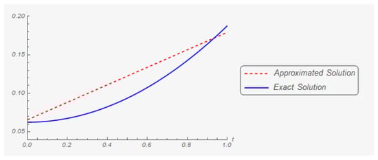
Figure 1. The first component of the exact solution and its first approximation.

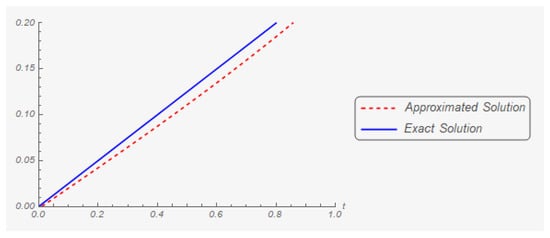
Figure 2. The second component of the exact solution and its first approximation.

Also, for the first iteration, the maximum deviations of the exact solution are

$$\underset{t\in \left[0,1\right]}{max}\left|x_1^{*}\left(t\right)-x_{11}\left(t\right)\right|\le 0.02893$$

$$\underset{t\in \left[0,1\right]}{max}\left|x_2^{*}\left(t\right)-x_{12}\left(t\right)\right|\le 0.01547$$

Similarly, we use (41) and (42) to find the unknown parameters for each iteration. Also, for each iteration the solutions of approximate systems are so close with (50)–(53). Therefore, for the next iterations, components of exact and approximate solutions are shown by figures and with their maximum errors.

Iteration 50: The graphs of the first and second components of the exact and approximate (in the fifth iteration) solutions are shown in Figure 3 and Figure 4 respectively.

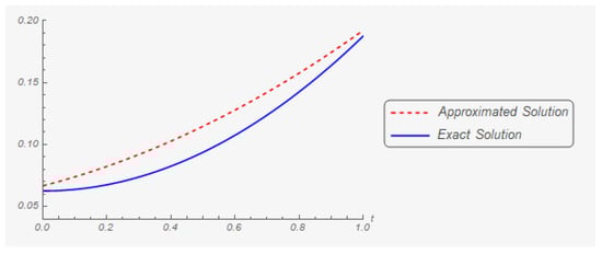
Figure 3. The first component of the exact solution and its fifth approximation.

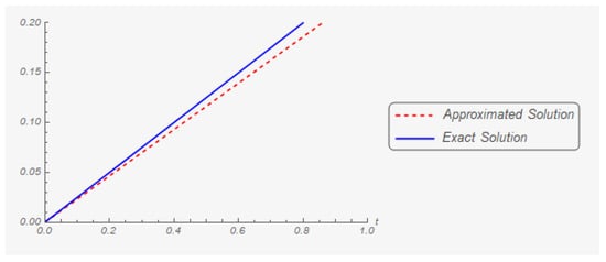
Figure 4. The second component of the exact solution and its fifth approximation.

The following inequalities are related to the maximum deviation of the exact solution with its fifth approximations.

$$\underset{t\in \left[0,1\right]}{max}\left|x_1^{*}\left(t\right)-x_{501}\left(t\right)\right|\le 0.02096$$

$$\underset{t\in \left[0,1\right]}{max}\left|x_2^{*}\left(t\right)-x_{502}\left(t\right)\right|\le 0.01744$$

Iteration 100: The graphs of the first and second components of the exact and approximate (in the hundredth iteration) solutions are shown in Figure 5 and Figure 6 respectively.

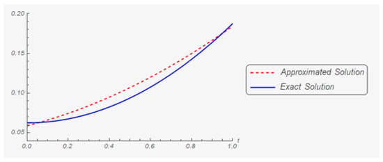
Figure 5. The first component of the exact solution and its hundredth approximation.

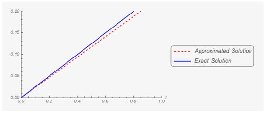
Figure 6. The second component of the exact solution and its hundredth approximation.

For the hundredth approximation the maximum deviations of the exact solution are

$$\underset{t\in \left[0,1\right]}{max}\left|x_1^{*}\left(t\right)-x_{1001}\left(t\right)\right|\le 0.01311$$

$$\underset{t\in \left[0,1\right]}{max}\left|x_2^{*}\left(t\right)-x_{1002}\left(t\right)\right|\le 0.01471$$

Iteration 150: The graphs of the first and second components of the exact and approximate (in the one hundred and fifth iteration) solutions are shown on Figure 7 and Figure 8 respectively.

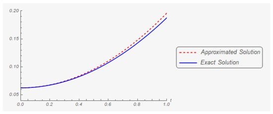
Figure 7. The first component of the exact solution and its one hundred and fifth approximation.

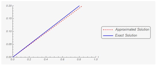
Figure 8. The second component of the exact solution and its one hundred and fifth approximation.

The following inequalities are related with the maximum deviations of the exact solution with its one hundred and fifth approximations.

$$\underset{t\in \left[0,1\right]}{max}\left|x_1^{*}\left(t\right)-x_{1501}\left(t\right)\right|\le 0.008333$$

$$\underset{t\in \left[0,1\right]}{max}\left|x_2^{*}\left(t\right)-x_{1502}\left(t\right)\right|\le 0.01077$$

Iteration 200: The graphs of the first and second components of the exact and approximate (in the two hundredth iteration) solutions are shown in Figure 9 and Figure 10, respectively.

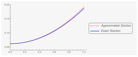
Figure 9. The first component of the exact solution and its two hundredth approximation.

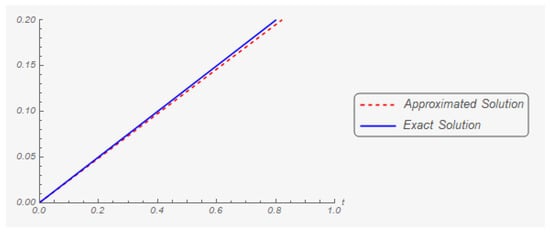
Figure 10. The second component of the exact solution and its two hundredth approximation.

For the two hundredth iteration, the maximum deviations of the exact solution are

$$\underset{t\in \left[0,1\right]}{max}\left|x_1^{*}\left(t\right)-x_{2001}\left(t\right)\right|\le 0.00487$$

$$\underset{t\in \left[0,1\right]}{max}\left|x_2^{*}\left(t\right)-x_{2002}\left(t\right)\right|\le 0.006097$$

Iteration 250: The graphs of the first and second components of the exact and approximate (in the two hundredth and fifth iteration) solutions are shown in Figure 11 and Figure 12, respectively.

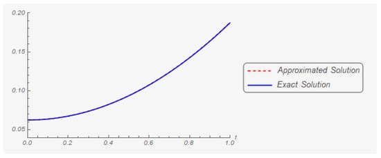
Figure 11. The first component of the exact solution and its two hundredth and fifth approximation.

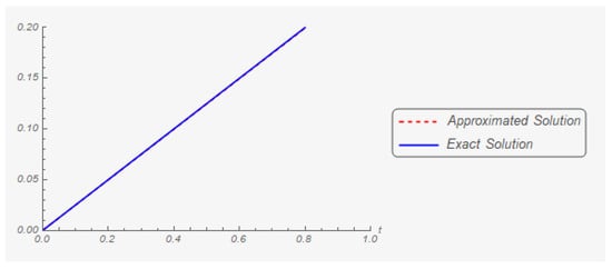
Figure 12. The second component of the exact solution and its two hundredth and fifth approximation.

The following inequalities are related with the maximum deviations of the exact solution with its two hundredth and fifth approximations

$$\underset{t\in \left[0,1\right]}{max}\left|x_1^{*}\left(t\right)-x_{2501}\left(t\right)\right|\le 0.0004704$$

$$\underset{t\in \left[0,1\right]}{max}\left|x_2^{*}\left(t\right)-x_{2502}\left(t\right)\right|\le 0.0006233$$

Iteration 300: The graphs of the first and second components of the exact and approximate (in the three hundredth iteration) solutions are shown in Figure 13 and Figure 14, respectively.

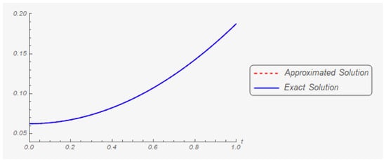
Figure 13. The first component of the exact solution and its three hundredth approximation.

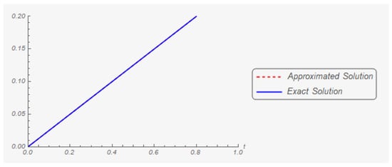
Figure 14. The second component of the exact solution and its three hundredth approximation.

The following inequalities are related with the maximum deviations of the exact solution with its three hundredth approximations.

$$\underset{t\in \left[0,1\right]}{max}\left|x_1^{*}\left(t\right)-x_{3001}\left(t\right)\right|\le 0.00007809$$

$$\underset{t\in \left[0,1\right]}{max}\left|x_2^{*}\left(t\right)-x_{3002}\left(t\right)\right|\le 0.00006241$$

Iteration 364: The graphs of the first and second components of the exact and approximate (in the three hundred and sixty-fourth iteration) solutions are shown in Figure 15 and Figure 16, respectively.

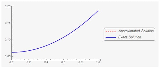
Figure 15. The first component of the exact solution and its three hundred and sixty-fourth approximation.

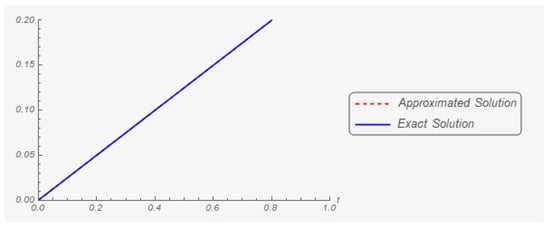
Figure 16. The second component of the exact solution and its three hundred and sixty-fourth approximation.

The following inequalities are related with the maximum deviations of the exact solution with its three hundred and sixty-fourth approximations.

$$\underset{t\in \left[0,1\right]}{max}\left|x_1^{*}\left(t\right)-x_{1001}\left(t\right)\right|\le 1.209\times {10}^{-6}$$

$$\underset{t\in \left[0,1\right]}{max}\left|x_2^{*}\left(t\right)-x_{1002}\left(t\right)\right|\le 5.813\times {10}^{-6}$$

The results of the 1st component of the exact solution and its 1st approximation are compared for some t values in Table 1 with errors.

Table 1. Comparing approximated and first component of exact Solution with error.

t	Exact Solution	Approximated Solution	Error	Relative Errors
0.1	0.06375	0.07704	0.01329	0.2085
0.2	0.0675	0.08838	0.02088	0.3093
0.3	0.07375	0.09973	0.02598	0.3523
0.4	0.0825	0.1111	0.02857	0.3467
0.5	0.09375	0.1224	0.02867	0.3056
0.6	0.1075	0.1338	0.02626	0.2447
0.7	0.1238	0.1451	0.02135	0.1721
0.8	0.1425	0.1564	0.01395	0.0975
0.9	0.1638	0.1678	0.00404	0.0244
1	0.1875	0.1791	0.008367	0.0448

The results of the second component of the exact solution and its 1st approximation are compared for some t values in Table 2 with errors.

Table 2. Comparing Approximated and second component of exact solution with error.

t	Exact Solution	Approximated Solution	Error	Relative Errors
0.1	0.025	0.01992	0.005082	0.2032
0.2	0.05	0.04215	0.007847	0.1570
0.3	0.075	0.06464	0.01036	0.1381
0.4	0.1	0.08749	0.01251	0.1251
0.5	0.125	0.1108	0.01416	0.1136
0.6	0.15	0.1348	0.01518	0.1013
0.7	0.175	0.1595	0.01546	0.0886
0.8	0.2	0.1851	0.01487	0.0745
0.9	0.225	0.2117	0.01328	0.0591
1	0.25	0.2394	0.01056	0.0424

The results of the 1st component of the exact solution and its last approximation are compared for some t values in Table 3 with errors.

Table 3. Comparing Approximated and first component of exact solutions with error.

t	Exact Solution	Approximated Solution	Error	Relative Errors
0.1	0.06375	0.06375	1.563 × 10−8	2.418 × 10−7
0.2	0.0675	0.0675	6.25 × 10−8	9.2593 × 10−7
0.3	0.07375	0.07375	1.406 × 10−7	1.9064 × 10−6
0.4	0.0825	0.0825	0.00000025	3.0303 × 10−6
0.5	0.09375	0.09375	3.906 × 10−7	4.1664 × 10−6
0.6	0.1075	0.1075	5.625 × 10−7	5.2326 × 10−6
0.7	0.1238	0.1238	7.656 × 10−7	6.1842 × 10−6
0.8	0.1425	0.1425	0.000001	7.0175 × 10−6
0.9	0.1638	0.1638	0.000001266	7.7289 × 10−6
1	0.1875	0.1875	0.000001563	8.3360 × 10−6

Note that, for example, 1.563 × 10⁻⁸ means to multiply 1.563 by 0.00000001. The results of the second component of the exact solution and its last approximation are compared for some t values in Table 4 with errors.

Table 4. Comparing Approximated and second component of exact Solutions with error.

t	Exact Solution	Approximated Solution	Error	Relative Errors
0.1	0.025	0.025	0.000000625	2.5000 × 10−5
0.2	0.05	0.05	0.00000125	2.5000 × 10−5
0.3	0.075	0.075	0.000001875	2.5000 × 10−5
0.4	0.1	0.1	0.0000025	2.5000 × 10−5
0.5	0.125	0.125	0.000003125	2.5000 × 10−5
0.6	0.15	0.15	0.00000375	2.5000 × 10−5
0.7	0.175	0.175	0.000004375	2.5000 × 10−5
0.8	0.2	0.2	0.000005	2.5000 × 10−5
0.9	0.225	0.225	0.000005625	2.5000 × 10−5
1	0.25	0.25	0.00000625	2.5000 × 10−5

7. Conclusions

In this article, we studied Caputo-type fractional differential equations with parametrized boundary conditions. To study of the solution of the Caputo-type fractional differential equation, successive approximations are considered. It is shown that these successive approximations are uniformly convergent and the relationship between the limit function and the exact solution of the boundary-value problem is stated.

References

- Ahmad, B.; Ntouyas, S.K.; Tariboon, J. Nonlocal fractional-order boundary value problems with generalized Riemann-Liouville integral boundary conditions. J. Comp. Anal. Appl. 2017, 23, 1281–1296. [Google Scholar]
- Ahmad, B. Existence of solutions for fractional differential equations of order q∈(2, 3] with anti-periodic boundary conditions. J. Appl. Math. Comput. 2010, 34, 385–391. [Google Scholar] [CrossRef]
- Mahmudov, N.; Emin, S. Fractional-order boundary value problems with Katugampola fractional integral conditions. Adv. Differ. Equ. 2018, 2018, 81. [Google Scholar] [CrossRef]
- Marynets, K. On construction of the approximate solution of the special type integral boundary-value problem. Electron. J. Qual. Theory Differ. Equ. 2016, 6, 1–14. [Google Scholar] [CrossRef]
- Ronto, M.I.; Marynets, K.V. On the parametrization of boundary-value problems with two-point nonlinear boundary conditions. Nonlinear Oscil. 2012, 14, 379–413. [Google Scholar] [CrossRef]
- Ronto, M.; Marynets, K.V.; Varha, J.V. Further results on the investigation of solutions of integral boundary value problems. Tatra Mt. Math. Publ. 2015, 63, 247–267. [Google Scholar] [CrossRef][Green Version]
- Ronto, A.; Ronto, M. Periodic successive approximations and interval halving. Miskolc Math. Notes 2012, 13, 459–482. [Google Scholar] [CrossRef]
- Ronto, M.; Samoilenko, A.M. Numerical-Analytic Methods in the Theory of Boundary-Value Problems; World Scientific: Singapore, 2000. [Google Scholar]
- Fečkan, M.; Marynets, K. Approximation approach to periodic BVP for fractional differential systems. Eur. Phys. J. 2017, 226, 3681–3692. [Google Scholar] [CrossRef]
- Fečkan, M.; Marynets, K. Approximation approach to periodic BVP for mixed fractional differential systems. J. Comput. Appl. Math. 2018, 339, 208–217. [Google Scholar] [CrossRef]
- Ronto, M.; Marynets, K. Parametrization for Nonlinear problems with integral boundary conditions. Electron. J. Qual. Theory Differ. Equ. 2012, 99, 1–23. [Google Scholar] [CrossRef]
- Batelli, F.; Fečkan, M. Hand Book of Differential Equations: Ordinary Differential Equations; Elsevier: Amsterdam, The Netherlands, 2008. [Google Scholar]
© 2019 by the authors. Licensee MDPI, Basel, Switzerland. This article is an open access article distributed under the terms and conditions of the Creative Commons Attribution (CC BY) license (http://creativecommons.org/licenses/by/4.0/).