Modified Proximal Algorithms for Finding Solutions of the Split Variational Inclusions

Abstract

We investigate the split variational inclusion problem in Hilbert spaces. We propose efficient algorithms in which, in each iteration, the stepsize is chosen self-adaptive, and proves weak and strong convergence theorems. We provide numerical experiments to validate the theoretical results for solving the split variational inclusion problem as well as the comparison to algorithms defined by Byrne et al. and Chuang, respectively. It is shown that the proposed algorithms outrun other algorithms via numerical experiments. As applications, we apply our method to compressed sensing in signal recovery. The proposed methods have as a main advantage that the computation of the Lipschitz constants for the gradient of functions is dropped in generating the sequences.

1. Introduction

Let H be a real Hilbert space. Then, $B:H\to 2^H$ is called monotone if $\langle u-v,x-y\rangle \ge 0$ for each $u\in Bx$, $v\in By$. Moreover, B is maximal monotone provided its graph is not properly included in the graph of other monotone mappings. Many problems in optimization can be reduced to finding $x^{*}\in H$ such that $0\in B{x}^{*}$. Martinet [1] and Rockafellar [2] suggested the proximal method for solving this problem. They construct the sequence $\{x_n\}\subset H$ by choosing $x_1\in H$ and putting

$$x_{n+1}=J_{{\beta }_n}^B{x}_n,n\in \mathbb{N},$$

(1)

where $\{{\beta }_n\}\subseteq (0,\infty )$, B is a set-valued maximal monotone operator and $J_{\beta }^B$ is defined by $J_{\beta }^B={(I+\beta B)}^{-1}$ for each $\beta >0$. We see that Equation (1) is equivalent to $x_n-x_{n+1}\in {\beta }_{n}B{x}_{n+1}$, $n\in \mathbb{N}$.

The split variational inclusion problem (SVIP) was first investigated by Moudafi [3]. The problem consists of finding $x^{*}\in H_1$ such that

$$0\in B_1(x^{*})\mathrm{and}0\in B_2(A{x}^{*}),$$

(2)

where $H_1$ and $H_2$ are real Hilbert spaces, $B_1$ and $B_2$ are set-valued mappings on $H_1$ and $H_2$. In addition, $A:H_1\to H_2$ is a bounded and linear operator and $A^{*}$ is the adjoint of A. We know that the SVIP is a generalization of the split feasibility problem that was investigated by Censor and Elfving [4] in Euclidean spaces. See [4,5,6,7,8,9]. In this paper, we denote by $\Omega$ the solution set of SVIP. Suppose that $\Omega$ is nonempty.

In 2011, Byrne et al. [6] established a weak convergence theorem for SVIP as follows:

Theorem 1.

Let $H_1$ and $H_2$ be real Hilbert spaces, $A:H_1\to H_2$ be a bounded linear operator. Let $B_1:H_1\to 2^{H_1}$ and $B_2:H_2\to 2^{H_2}$ be set-valued maximal monotone operators. Let $\beta >0$ and $\gamma \in (0,\frac{2}{{\parallel A\parallel }^2})$. Let $\{x_n\}$ be generated by

$$x_{n+1}=J_{\beta }^{B_1}(x_n-\gamma A^{*}(I-J_{\beta }^{B_2})A{x}_n),n\in \mathbb{N}.$$

(3)

Then, $\{x_n\}$ converges weakly to $x^{*}$ in Ω.

In 2015, Chuang [10] introduced the following iteration for SVIP in Hilbert spaces.

Chuang [10] established its convergence as follows:

Theorem 2.

Let $H_1$ and $H_2$ be real Hilbert spaces, $A:H_1\to H_2$ be a bounded and linear operator. Let $B_1:H_1\to 2^{H_1}$ and $B_2:H_2\to 2^{H_2}$ be set-valued maximal monotone operators. Choose $\delta \in (0,1)$ and let $\{{\beta }_n\}\subseteq (0,\infty )$ and $\{{\gamma }_n\}\subseteq (0,\frac{\delta }{{\parallel A\parallel }^2})$ and assume that

$$\sum _{n=1}^{\infty }{\gamma }_n=\infty ,\sum _{n=1}^{\infty }{\gamma }_n^2<\infty ,\underset{n\to \infty }{lim\; inf}{\beta }_n>0.$$

(4)

If $H_1$ is finite dimensional, then ${lim}_{n\to \infty }{x}_n=x^{*}\in \Omega$.

Chuang [10] also provided the following result.

Theorem 3.

Let $H_1$ and $H_2$ be infinite dimensional Hilbert spaces, $A:H_1\to H_2$ be a bounded and linear operator. Let $B_1:H_1\to 2^{H_1}$ and $B_2:H_2\to 2^{H_2}$ be set-valued maximal monotone mappings. Choose $\delta \in (0,1)$ and let $\{{\beta }_n\}\subseteq (0,\infty )$, ${lim\; inf}_{n\to \infty }{\beta }_n>0$ and $\{{\gamma }_n\}\subseteq (0,\frac{\delta }{{\parallel A\parallel }^2})$ with ${inf}_{n\in \mathbb{N}}{\gamma }_n>0$. Then, $x_n\to x^{*}\in \Omega$.

In 2013, Chuang [11] proved strong convergence theorem for SVIP using the following algorithm.

Algorithm 1:

[11].  For $n\in \mathbb{N}$, set $y_n$ as $$y_n=J_{{\beta }_n}^{B_1}(x_n-{\gamma }_n{A}^{*}(I-J_{{\beta }_n}^{B_2})A{x}_n),$$ (5)  where ${\gamma }_n>0$ is chosen such that $${\gamma }_n\parallel A^{*}(I-J_{{\beta }_n}^{B_2})A{x}_n-A^{*}(I-J_{{\beta }_n}^{B_2})A{y}_n\parallel \le \delta \parallel x_n-y_n\parallel ,0<\delta <1.$$ (6)  The iterative $x_{n+1}$ is generated by $$x_{n+1}=J_{{\beta }_n}^{B_1}(x_n-{\alpha }_{n}D(x_n,{\gamma }_n)),$$ (7)  where $$D(x_n,{\gamma }_n)=x_n-y_n+{\gamma }_n(A^{*}(I-J_{{\beta }_n}^{B_2})A{y}_n-A^{*}(I-J_{{\beta }_n}^{B_2})A{x}_n)$$ (8)  and $${\alpha }_n=\frac{\langle x_n-y_n,D(x_n,{\gamma }_n)\rangle }{\parallel D(x_n,{\gamma }_n){\parallel }^2}.$$ (9)

Theorem 4.

Let $H_1$ and $H_2$ be two real Hilbert spaces, $A:H_1\to H_2$ be a bounded and linear operator. Let $B_1:H_1\to 2^{H_1}$ and $B_2:H_2\to 2^{H_2}$ be two set-valued maximal monotone operators. Let $\{a_n\}$, $\{b_n\}$, $\{c_n\}$, and $\{d_n\}$ be sequences of real numbers in $[0,1]$ with $a_n+b_n+c_n+d_n=1$ and $0<a_n<1$ for each $n\in \mathbb{N}$. Let $\{{\beta }_n\}\subseteq (0,\infty )$ and let $\{{\gamma }_n\}\subseteq (0,\frac{2}{{\parallel A\parallel }^2+1})$. Let $\{v_n\}$ be a bounded sequence in $H_1$. Fix $u\in H_1$ and let the sequence $\{x_n\}\subseteq H_1$ be generated by

$$x_{n+1}=a_{n}u+b_n{x}_n+c_n{J}_{{\beta }_n}^{B_1}(x_n-{\gamma }_n{A}^{*}(I-J_{{\beta }_n}^{B_2})A{x}_n)+d_n{v}_n$$

(10)

for each $n\in \mathbb{N}$. Suppose that

(i) 

${lim}_{n\to \infty }{a}_n={lim}_{n\to \infty }\frac{d_n}{a_n}=0$; ${\sum }_{n=1}^{\infty }{a}_n=\infty$; ${\sum }_{n=1}^{\infty }{d}_n<\infty$;

(ii) 

${lim\; inf}_{n\to \infty }{c}_n{\gamma }_n>0$, ${lim\; inf}_{n\to \infty }{b}_n{c}_n>0$, ${lim\; inf}_{n\to \infty }{\beta }_n>0$.

Then, ${lim}_{n\to \infty }{x}_n=x^{*}$, where $x^{*}=P_{\Omega }u$ and $P_{\Omega }u$ is nearest to u.

We aim to find the approximate algorithms with a new step size which is self-adaptive (see López et al. [8]) for solving our SVIP and prove its convergence. We present numerical examples and the comparison to algorithms of Byne et al. [6] and algorithms of Chuang [10,11]. We also obtain the result for split feasibility problem (SFP) and its applications to compressed sensing in signal recovery. It reveals that our methods have a better convergence than those of Byrne et al. [6] and Chuang [10,11].

2. Preliminaries

We next provide some basic concepts for our proof. In what follows, we shall use the following symbols:

• ⇀ stands for the weak convergence,
• → stands for the strong convergence.

Recall that a mapping $T:H\to H$ is called

(1)

nonexpansive if, for all $x,y\in H$,

$$\parallel Tx-Ty\parallel \le \parallel x-y\parallel .$$

(11)

(2)

firmly-nonexpansive if, for all $x,y\in H$,

$${\parallel Tx-Ty\parallel }^2\le \langle Tx-Ty,x-y\rangle .$$

(12)

It is clear that $I-T$ is also firmly-nonexpansive when T is firmly-nonexpansive. We know that, for each $x,y\in H$,

$$\langle x,y\rangle =\frac{1}{2}{\parallel x\parallel }^2+\frac{1}{2}{\parallel y\parallel }^2-\frac{1}{2}{\parallel x-y\parallel }^2$$

(13)

and

$${\parallel tx+(1-t)y\parallel }^2={t\parallel x\parallel }^2+{(1-t)\parallel y\parallel }^2-t(1-t){\parallel x-y\parallel }^2$$

(14)

for all $x,y\in H$ and for all $t\in [0,1]$.

The following lemma can be found in [12].

Lemma 1.

Let C be a nonempty closed convex subset of a real Hilbert space H. Let $T:C\to C$ be a nonexpansive mapping. If $x_n\rightharpoonup x\in C$ and ${\displaystyle \underset{n\to \infty }{lim}\parallel x_n-T{x}_n\parallel =0}$, then $x=Tx$.

We use $Fix(T)$ by the fixed point set of a mapping T, that is, $Fix(T)=\{x\in H:x=Tx\}$ and $D(T)$ by the domain of a mapping T, i.e., $D(T)=\{x\in H:T(x)\ne \varnothing \}$.

The following lemma can be found in [11,13].

Lemma 2.

Let H be a real Hilbert space and let $B:H\to 2^H$ be a maximal monotone operator. Then,

(i) 

$J_{\beta }^B$ is single-valued and firmly nonexpansive for each $\beta >0$;

(ii) 

$\mathcal{D}(J_{\beta }^B)=H$ and $Fix(J_{\beta }^B)=\{x\in \mathcal{D}(B):0\in Bx\}$;

(iii) 

$\parallel x-J_{\beta }^{B}x\parallel \le \parallel x-J_{\gamma }^{B}x\parallel$ for all $0<\beta \le \gamma$ and for all $x\in H$;

(iv) 

If $B^{-1}(0)\ne \varnothing$, then we have $\parallel x-J_{\beta }^B{x\parallel }^2+\parallel J_{\beta }^{B}x-x^{*}{\parallel }^2\le {\parallel x-x^{*}\parallel }^2$ for all $x\in H$, each $x^{*}\in B^{-1}(0)$, and each $\beta >0$;

(v) 

If $B^{-1}(0)\ne \varnothing$, then we have $\langle x-J_{\beta }^{B}x,J_{\beta }^{B}x-w\rangle \ge 0$ for all $x\in H$, each $w\in B^{-1}(0)$, and each $\beta >0$.

Lemma 3.

Let $H_1$ and $H_2$ be real Hilbert spaces. Let $A:H_1\to H_2$ be a bounded and linear operator. Let $\beta >0$, $\gamma >0$, $B_1:H_1\to 2^{H_1}$ and $B_2:H_2\to 2^{H_2}$ be maximal monotone operators. Let $x^{*}\in H_1$.

(i) 

If $x^{*}$ is a solution of (SVIP), then $J_{\beta }^{B_1}(x^{*}-\gamma A^{*}(I-J_{\beta }^{B_2})A{x}^{*})=x^{*}$.

(ii) 

Suppose that $J_{\beta }^{B_1}(x^{*}-\gamma A^{*}(I-J_{\beta }^{B_2})A{x}^{*})=x^{*}$ and the solution set of (SVIP) is nonempty. Then, $x^{*}$ is a solution of (SVIP).

Lemma 4.

Let $H_1$ and $H_2$ be real Hilbert spaces. Let $A:H_1\to H_2$ be a bounded and linear operator and $\beta >0$. Let $B:H_2\to 2^{H_2}$ be a maximal monotone operator. Define a mapping $T:H_1\to H_1$ by $Tx:=A^{*}(I-J_{\beta }^B)Ax$ for each $x\in H_1$. Then,

(i) 

$\parallel (I-J_{\beta }^B)Ax-(I-J_{\beta }^B){Ay\parallel }^2\le \langle Tx-Ty,x-y\rangle$ for all $x,y\in H_1$;

(ii) 

$\parallel A^{*}(I-J_{\beta }^B)Ax-A^{*}(I-J_{\beta }^B){Ay\parallel }^2\le {\parallel A\parallel }^2·\langle Tx-Ty,x-y\rangle$ for all $x,y\in H_1$.

The following lemma can be found in [14].

Lemma 5.

Let C be a nonempty subset of a Hilbert space H. Let $\{x_n\}$ be a sequence in H that satisfies the following assumptions:

(i) 

${\displaystyle \underset{n\to \infty }{lim}\parallel x_n-x\parallel }$ exists for each $x\in C$;

(ii) 

every sequential weak limit point of $\{x_n\}$ is in C.

Then, $\{x_n\}$ weakly converges to a point in C.

The following lemma can be found in [15].

Lemma 6.

Assume $\{s_n\}\subseteq (0,\infty )$ such that

$$\begin{array}{ccc}\hfill s_{n+1}& \le & (1-{\alpha }_n)s_n+{\alpha }_n{\delta }_n,n\ge 1,\hfill \end{array}$$

(15)

$$\begin{array}{ccc}\hfill s_{n+1}& \le & s_n-{\lambda }_n+{\phi }_n,n\ge 1,\hfill \end{array}$$

(16)

where $\{{\alpha }_n\}\subseteq (0,1)$, $\{{\lambda }_n\}\subseteq (0,1)$ and $\{{\delta }_n\}$ and $\{{\phi }_n\}$ are real sequences such that

(i) 

${\displaystyle \sum _{n=1}^{\infty }{\alpha }_n=\infty }$;

(ii) 

${\displaystyle \underset{n\to \infty }{lim}{\phi }_n=0}$;

(iii) 

${lim}_{k\to \infty }{\lambda }_{n_k}=0$ implies ${\displaystyle \underset{k\to \infty }{lim\; sup}{\delta }_{n_k}\le 0}$ for any subsequence $\{n_k\}$ of $\{n\}$.

Then, ${\displaystyle \underset{n\to \infty }{lim}{s}_n=0}$.

3. Weak Convergence Result

Let, $H_1$ and $H_2$ be real Hilbert spaces, $A:H_1\to H_2$ be a bounded and linear operator. Let $B_1:H_1\to 2^{H_1}$ and $B_2:H_2\to 2^{H_2}$ be set-valued maximal monotone operators.

Let $\Omega$ be a solution set of problem (SVIP) and assume that $\Omega \ne \varnothing$. We remark that the stepsize sequence $\{{\gamma }_n\}$ does not depend on the norm of an operator A as introduced by Byrne et al. [6] and Chuang [10,11].

Theorem 5.

Suppose that ${\displaystyle \underset{n\to \infty }{lim\; inf}{\beta }_n>0}$, ${\displaystyle \underset{n}{inf}{\rho }_n(4-{\rho }_n)>0}$ and ${\displaystyle \underset{n\to \infty }{lim}{\theta }_n=0}$. Then, $\{x_n\}$ defined by Algorithm 2 converges weakly to a solution in Ω.

Algorithm 2:

Choose $x_1\in H_1$ and define $$x_{n+1}=J_{{\beta }_n}^{B_1}(x_n-{\gamma }_{n}g(x_n)),$$ (17)    where $${\gamma }_n=\frac{{\rho }_{n}f(x_n)}{\parallel g(x_n){\parallel }^2+{\theta }_n},0<{\rho }_n<4,0<{\theta }_n<1,{\beta }_n>0,$$ (18)    and $$f(x_n)=\frac{1}{2}{\parallel (I-J_{{\beta }_n}^{B_2})A{x}_n\parallel }^2,g(x_n)=A^{*}(I-J_{{\beta }_n}^{B_2})A{x}_n.$$ (19)

Proof. 

Let $z\in \Omega$. Then, $z\in B_1^{-1}(0)$ and $Az\in B_2^{-1}(0)$. Thus, we have $J_{{\beta }_n}^{B_2}Az=Az$. Using Lemma 4 (i), we have

$$\begin{array}{ccc}\hfill \langle x_n-z,g(x_n)\rangle & =& \langle x_n-z,g(x_n)-g(z)\rangle \hfill \\ & =& \langle x_n-z,A^{*}(I-J_{{\beta }_n}^{B_2})A{x}_n-A^{*}(I-J_{{\beta }_n}^{B_2})Az\rangle \hfill \\ & =& \langle A{x}_n-Az,(I-J_{{\beta }_n}^{B_2})A{x}_n-(I-J_{{\beta }_n}^{B_2})Az\rangle \hfill \\ & \ge & \parallel (I-J_{{\beta }_n}^{B_2})A{x}_n{\parallel }^2\hfill \\ & =& 2f(x_n).\hfill \end{array}$$

(20)

From Equation (20), Lemma 2 (iv) and the defining formulas for Algorithm 2

$$\begin{array}{ccc}\hfill \parallel x_{n+1}{-z\parallel }^2& =& \parallel J_{{\beta }_n}^{B_1}(x_n-{\gamma }_{n}g(x_n)){-z\parallel }^2\hfill \\ & \le & \parallel x_n-{\gamma }_{n}g(x_n){-z\parallel }^2-{\parallel x_{n+1}-x_n+{\gamma }_{n}g(x_n)\parallel }^2\hfill \\ & =& \parallel x_n{-z\parallel }^2+{\gamma }_n^2\parallel g(x_n){\parallel }^2-2{\gamma }_n\langle x_n-z,g(x_n)\rangle -{\parallel x_{n+1}-x_n+{\gamma }_{n}g(x_n)\parallel }^2\hfill \\ & \le & \parallel x_n{-z\parallel }^2+{\gamma }_n^2\parallel g(x_n){\parallel }^2-4{\gamma }_{n}f(x_n)-{\parallel x_{n+1}-x_n+{\gamma }_{n}g(x_n)\parallel }^2\hfill \\ & =& \parallel x_n{-z\parallel }^2+\frac{{\rho }_n^2{f}^2(x_n)}{(\parallel g(x_n){{\parallel }^2+{\theta }_n)}^2}{\parallel g(x_n)\parallel }^2-\frac{4{\rho }_n{f}^2(x_n)}{\parallel g(x_n){\parallel }^2+{\theta }_n}\hfill \\ & & -\parallel x_{n+1}-x_n+{\gamma }_{n}g(x_n){\parallel }^2\hfill \\ & \le & \parallel x_n{-z\parallel }^2+\frac{{\rho }_n^2{f}^2(x_n)}{\parallel g(x_n){\parallel }^2+{\theta }_n}-\frac{4{\rho }_n{f}^2(x_n)}{\parallel g(x_n){\parallel }^2+{\theta }_n}-{\parallel x_{n+1}-x_n+{\gamma }_{n}g(x_n)\parallel }^2\hfill \\ & =& \parallel x_n{-z\parallel }^2-{\rho }_n(4-{\rho }_n)\frac{f^2(x_n)}{\parallel g(x_n){\parallel }^2+{\theta }_n}-{\parallel x_{n+1}-x_n+{\gamma }_{n}g(x_n)\parallel }^2.\hfill \end{array}$$

(21)

This implies that, since $0<{\rho }_n<4$,

$$\parallel x_{n+1}-z\parallel \le \parallel x_n-z\parallel .$$

(22)

Thus, ${\displaystyle \underset{n\to \infty }{lim}\parallel x_n-z\parallel }$ exists. It follows that $\{x_n\}$ is bounded. Again, by Equation (21), we get

$${\displaystyle {\rho }_n(4-{\rho }_n)\frac{f^2(x_n)}{\parallel g(x_n){\parallel }^2+{\theta }_n}\le \parallel x_n{-z\parallel }^2-{\parallel x_{n+1}-z\parallel }^2,}$$

(23)

which yields by our assumptions that

$${\displaystyle \underset{n\to \infty }{lim}\frac{f^2(x_n)}{\parallel g(x_n){\parallel }^2}=0.}$$

(24)

By Lemma 3 (ii), it can be checked that g is a Lipschitzian mapping and thus $\{\parallel g(x_n)\parallel \}$ is bounded. Hence, we get ${\displaystyle \underset{n\to \infty }{lim}f(x_n)=0}$. This means

$${\displaystyle \underset{n\to \infty }{lim}\parallel (I-J_{{\beta }_n}^{B_2})A{x}_n\parallel =0.}$$

(25)

Furthermore, by Equation (21), we also have

$${\displaystyle \underset{n\to \infty }{lim}\parallel x_{n+1}-x_n+{\gamma }_{n}g(x_n)\parallel =0.}$$

(26)

We note that

$${\displaystyle {\gamma }_n\parallel g(x_n)\parallel =\frac{{\rho }_{n}f(x_n)}{\parallel g(x_n){\parallel }^2+{\theta }_n}\parallel g(x_n)\parallel \to 0,\mathrm{as}n\to \infty .}$$

(27)

Hence, by Equations (26) and (27), we obtain

$${\displaystyle \underset{n\to \infty }{lim}\parallel x_{n+1}-x_n\parallel =0.}$$

(28)

From Equation (25) and Lemma 2 (iii), we get

$$\underset{n\to \infty }{lim}\parallel A{x}_n-J_{\beta }^{B_2}A{x}_n\parallel \le \underset{n\to \infty }{lim}\parallel A{x}_n-J_{{\beta }_n}^{B_2}A{x}_n\parallel =0,$$

(29)

for some $\beta >0$ such that ${\beta }_n\ge \beta >0$ for all $n\in \mathbb{N}$. From Equation (27), we see that

$$\begin{array}{ccc}\hfill \parallel x_{n+1}-J_{{\beta }_n}^{B_2}{x}_n\parallel & =& \parallel J_{{\beta }_n}^{B_1}(x_n-{\gamma }_{n}g(x_n))-J_{{\beta }_n}^{B_1}{x}_n\parallel \hfill \\ & \le & \parallel x_n-{\gamma }_{n}g(x_n)-x_n\parallel \hfill \\ & =& {\gamma }_n\parallel g(x_n)\parallel \hfill \\ & \to & 0\mathrm{as}n\to \infty .\hfill \end{array}$$

(30)

From Equations (28) and (30), we have

$$\begin{array}{ccc}\hfill \parallel x_n-J_{{\beta }_n}^{B_1}{x}_n\parallel & =& \parallel x_n-x_{n+1}+x_{n+1}-J_{{\beta }_n}^{B_1}{x}_n\parallel \hfill \\ & \le & \parallel x_n-x_{n+1}\parallel +\parallel x_{n+1}-J_{{\beta }_n}^{B_1}{x}_n\parallel \hfill \\ & \to & 0\mathrm{as}n\to \infty .\hfill \end{array}$$

(31)

Lemma 2 (iii) gives

$$\underset{n\to \infty }{lim}\parallel x_n-J_{\beta }^{B_1}{x}_n\parallel \le \underset{n\to \infty }{lim}\parallel x_n-J_{{\beta }_n}^{B_1}{x}_n\parallel =0.$$

(32)

Since $\{x_n\}$ is bounded, there is a subsequence $\{x_{n_k}\}$ of $\{x_n\}$ and $x^{*}\in H_1$ with $x_{n_k}\rightharpoonup x^{*}$. We also have $A{x}_{n_k}\rightharpoonup A{x}^{*}$. By Equations (29) and (32), Lemmas 1 and 2 (ii), we obtain $x^{*}\in \Omega$. Using Lemma 5, we obtain that $\{x_n\}$ converges weakly to a solution in $\Omega$. □

4. Strong Convergence Result

Theorem 6.

Assume that $\{{\alpha }_n\}$, $\{{\rho }_n\}$ and $\{{\theta }_n\}$ satisfy the assumptions:

(a1) 

${\displaystyle \underset{n\to \infty }{lim}{\alpha }_n=0}$ and ${\displaystyle \sum _{n=1}^{\infty }{\alpha }_n=\infty }$;

(a2) 

${\displaystyle \underset{n}{inf}{\rho }_n(4-{\rho }_n)>0}$;

(a3) 

${\displaystyle \underset{n\to \infty }{lim}{\theta }_n=0}$;

(a4) 

${\displaystyle \underset{n\to \infty }{lim\; inf}{\beta }_n>0}$.

Then, $\{x_n\}$ defined by Algorithm 3 converges strongly to $z=P_{\Omega }u$ and $P_{\Omega }u$ is closest to u.

Algorithm 3:

Choose $x_1\in H_1$ and let $u\in H_1$. Let $\{{\alpha }_n\}$ be a real sequence in $(0,1)$. Let $\{x_n\}$ be iteratively   generated by $$x_{n+1}={\alpha }_{n}u+(1-{\alpha }_n)J_{{\beta }_n}^{B_1}(x_n-{\gamma }_{n}g(x_n)),$$ (33)   where $${\gamma }_n=\frac{{\rho }_{n}f(x_n)}{\parallel g(x_n){\parallel }^2+{\theta }_n},0<{\rho }_n<4,0<{\theta }_n<1,{\beta }_n>0$$ (34)   and $$f(x_n)=\frac{1}{2}{\parallel (I-J_{{\beta }_n}^{B_2})A{x}_n\parallel }^2,g(x_n)=A^{*}(I-J_{{\beta }_n}^{B_2})A{x}_n.$$ (35)

Proof. 

Set $z=P_{\Omega }u\in \Omega$. Using the line of proof as for Theorem 5, we have

$$\begin{array}{ccc}\hfill \parallel J_{{\beta }_n}^{B_1}(x_n-{\gamma }_{n}g(x_n)){-z\parallel }^2& \le & \parallel x_n{-z\parallel }^2-{\rho }_n(4-{\rho }_n)\frac{f^2(x_n)}{\parallel g(x_n){\parallel }^2+{\theta }_n}\hfill \\ & & -\parallel J_{{\beta }_n}^{B_1}(x_n-{\gamma }_{n}g(x_n))-x_n+{\gamma }_{n}g(x_n){\parallel }^2.\hfill \end{array}$$

(36)

Then,

$$\begin{array}{ccc}\hfill \parallel x_{n+1}{-z\parallel }^2& =& \parallel {\alpha }_n(u-z)+(1-{\alpha }_n)(J_{{\beta }_n}^{B_1}(x_n-{\gamma }_{n}g(x_n))-z){\parallel }^2\hfill \\ & \le & (1-{\alpha }_n){\parallel J_{{\beta }_n}^{B_1}(x_n-{\gamma }_{n}g(x_n))-z\parallel }^2+2{\alpha }_n\langle u-z,x_{n+1}-z\rangle .\hfill \end{array}$$

(37)

Combining Equations (36) and (37), we get

$$\begin{array}{ccc}\hfill \parallel x_{n+1}{-z\parallel }^2& \le & (1-{\alpha }_n){\parallel x_n-z\parallel }^2-(1-{\alpha }_n){\rho }_n(4-{\rho }_n)\frac{f^2(x_n)}{\parallel g(x_n){\parallel }^2+{\theta }_n}\hfill \\ & & -(1-{\alpha }_n){\parallel J_{{\beta }_n}^{B_1}(x_n-{\gamma }_{n}g(x_n))-x_n+{\gamma }_{n}g(x_n)\parallel }^2\hfill \\ & & +2{\alpha }_n\langle u-z,x_{n+1}-z\rangle .\hfill \end{array}$$

(38)

Next, we will show that $\{x_n\}$ is bounded. Again, using Equation (36),

$$\begin{array}{ccc}\hfill \parallel x_{n+1}-z\parallel & =& \parallel {\alpha }_{n}u+(1-{\alpha }_n)J_{{\beta }_n}^{B_1}(x_n-{\gamma }_{n}g(x_n))-z\parallel \hfill \\ & \le & {\alpha }_n\parallel u-z\parallel +(1-{\alpha }_n)\parallel x_n-z\parallel .\hfill \end{array}$$

(39)

Thus, $\{x_n\}$ is bounded. Employing Lemma 6, from Equation (38), we set

$$\begin{array}{ccc}\hfill s_n& =& \parallel x_n{-z\parallel }^2;\hfill \\ \hfill {\phi }_n& =& 2{\alpha }_n\langle u-z,x_{n+1}-z\rangle ;\hfill \\ \hfill {\delta }_n& =& 2\langle u-z,x_{n+1}-z\rangle ;\hfill \\ \hfill {\lambda }_n& =& (1-{\alpha }_n){\rho }_n(4-{\rho }_n)\frac{f^2(x_n)}{\parallel g(x_n){\parallel }^2+{\theta }_n}\hfill \\ & & +(1-{\alpha }_n){\parallel J_{{\beta }_n}^{B_1}(x_n-{\gamma }_{n}g(x_n))-x_n+{\gamma }_{n}g(x_n)\parallel }^2.\hfill \end{array}$$

(40)

Thus, Equation (38) reduces to the inequalities

$$\begin{array}{ccc}\hfill s_{n+1}& \le & (1-{\alpha }_n)s_n+{\alpha }_n{\delta }_n,n\ge 1,\hfill \end{array}$$

(41)

$$\begin{array}{ccc}\hfill s_{n+1}& \le & s_n-{\lambda }_n+{\phi }_n.\hfill \end{array}$$

(42)

Let $\{n_k\}\subseteq \{n\}$ be such that

$${\displaystyle \underset{k\to \infty }{lim}{\lambda }_{n_k}=0.}$$

(43)

Then, we have

$$\begin{array}{cc}{\displaystyle \underset{k\to \infty }{lim}}\hfill & ((1-{\alpha }_{n_k}){\rho }_{n_k}(4-{\rho }_{n_k})\frac{f^2(x_{n_k})}{\parallel g(x_{n_k}){\parallel }^2+{\theta }_{n_k}}\hfill \\ & +(1-{\alpha }_{n_k}){\parallel J_{{\beta }_{n_k}}^{B_1}(x_{n_k}-{\gamma }_{n_k}g(x_{n_k}))-x_{n_k}+{\gamma }_{n_k}g(x_{n_k})\parallel }^2)=0,\hfill \end{array}$$

(44)

which, by using our assumptions, implies

$${\displaystyle \frac{f_{n_k}^2(x_{n_k})}{\parallel g_{n_k}(x_{n_k}){\parallel }^2}\to 0\mathrm{as}k\to \infty ,}$$

(45)

and

$$\parallel J_{{\beta }_{n_k}}^{B_1}(x_{n_k}-{\gamma }_{n_k}g(x_{n_k}))-x_{n_k}+{\gamma }_{n_k}g(x_{n_k})\parallel \to 0\mathrm{as}k\to \infty .$$

(46)

Since $\{\parallel g_{n_k}(x_{n_k})\parallel \}$ is bounded, it follows that $f_{n_k}(x_{n_k})\to 0$ as $k\to \infty$. Thus, we get

$$\underset{k\to \infty }{lim}\parallel (I-J_{{\beta }_{n_k}}^{B_1})A{x}_{n_k}\parallel =0.$$

(47)

As the same proof in Theorem 5, we can show that there is $\{x_{n_{k_i}}\}$ of $\{x_{n_k}\}$ such that $x_{n_{k_i}}\rightharpoonup x^{*}\in \Omega$. From Lemma 2 (v), we obtain

$$\begin{array}{ccc}\hfill {\displaystyle \underset{k\to \infty }{lim\; sup}\langle u-z,x_{n_k}-z\rangle }& =& {\displaystyle \underset{i\to \infty }{lim}\langle u-z,x_{n_{k_i}}-z\rangle }\hfill \\ & =& \langle u-z,x^{*}-z\rangle \hfill \\ & \le & 0.\hfill \end{array}$$

(48)

We see that

$$\begin{array}{ccc}\hfill \parallel x_{n_k+1}-x_{n_k}\parallel & =& \parallel {\alpha }_{n_k}u+(1-{\alpha }_{n_k})J_{{\beta }_{n_k}}^{B_1}(x_{n_k}-{\gamma }_{n_k}g(x_{n_k}))-x_{n_k}\parallel \hfill \\ & \le & {\alpha }_{n_k}\parallel u-x_{n_k}\parallel +(1-{\alpha }_{n_k})\parallel J_{{\beta }_{n_k}}^{B_1}(x_{n_k}-{\gamma }_{n_k}g(x_{n_k}))-x_{n_k}\parallel \hfill \\ & \le & {\alpha }_{n_k}\parallel u-x_{n_k}\parallel +(1-{\alpha }_{n_k})\parallel J_{{\beta }_{n_k}}^{B_1}(x_{n_k}-{\gamma }_{n_k}g(x_{n_k}))-x_{n_k}+{\gamma }_{n_k}g(x_{n_k})\parallel \hfill \\ & & +(1-{\alpha }_{n_k}){\gamma }_{n_k}\parallel g(x_{n_k})\parallel \hfill \\ & \to & 0\mathrm{as}k\to \infty .\hfill \end{array}$$

(49)

From Equations (48) and (49), it follows that

$${\displaystyle \underset{k\to \infty }{lim\; sup}\langle u-z,x_{n_k+1}-z\rangle \le 0.}$$

(50)

Hence, we get

$${\displaystyle \underset{k\to \infty }{lim\; sup}{\delta }_{n_k}\le 0.}$$

(51)

Thus, $\{x_n\}$ converges strongly to $z=P_{\Omega }u$ by Lemma 6. □

5. Numerical Experiments

We present numerical experiments for our main results.

First, we give a comparison among Theorems 1–3 and 5 for a weak convergence theorem.

The following example is introduced in [10].

Example 1.

Let $B_1:{\mathbb{R}}^2\to {\mathbb{R}}^2$ and $B_2:{\mathbb{R}}^3\to {\mathbb{R}}^3$ be

$$A=\left[\begin{array}{cc}2& 1\\ 1& 2\\ 2& 2\end{array}\right],B_1\left[\begin{array}{c}x\\ y\end{array}\right]=\left[\begin{array}{cc}2& 2\\ 2& 2\end{array}\right]\left[\begin{array}{c}x\\ y\end{array}\right]+\left[\begin{array}{c}-2\\ -2\end{array}\right],B_2\left[\begin{array}{c}x\\ y\\ z\end{array}\right]=\left[\begin{array}{ccc}2& -2& -2\\ -2& 2& 2\\ -2& 2& 2\end{array}\right]\left[\begin{array}{c}x\\ y\\ z\end{array}\right].$$

(52)

We aim to find $x^{*}={(x_1^{*},x_2^{*})}^T\in {\mathbb{R}}^2$ such that $B_1(x^{*})={(0,0)}^T$ and $B_2(A{x}^{*})={(0,0,0)}^T$. In this case, we know that $x_1^{*}=1.5$ and $x_2^{*}=-0.5$.

We set ${\gamma }_n=0.001$ in Theorem 1, ${\gamma }_n=\frac{1}{{2n\parallel A\parallel }^2}$ in Theorem 2, ${\gamma }_n=\frac{\delta }{{2\parallel A\parallel }^2}$ in Theorem 3 and ${\gamma }_n=\frac{{\rho }_{n}f(x_n)}{\parallel g(x_n){\parallel }^2+{\theta }_n}$, ${\theta }_n=\frac{1}{n^5}$ in Theorem 5. The stopping criterion is given by $\parallel x_n-x^{*}{\parallel }_2<\epsilon$.

We test by the following cases:

Case 1:

$x_1=[1,1]$, ${\beta }_n=1$, ${\rho }_n=\frac{1.5n}{n+1}$, and $\delta =\frac{1}{3},$

Case 2:

$x_1=[4,-2]$, ${\beta }_n=2$, ${\rho }_n=\frac{3.5n}{n+1}$, and $\delta =\frac{1}{2},$

Case 3:

$x_1=[-5,-3]$, ${\beta }_n=3$, ${\rho }_n=2.8$, and $\delta =\frac{1}{4},$

Case 4:

$x_1=[-2,-7]$, ${\beta }_n=4$, ${\rho }_n=3.9$, and $\delta =\frac{1}{5}$.

From

Table 1. Comparison for Theorems 1–3 and 5 for each case.

	Method	$\mathit{\epsilon }={10}^{-4}$		$\mathit{\epsilon }={10}^{-5}$
		CPU	Iter	CPU	Iter
Case 1	Theorem 1	0.1091	3657	0.2763	7688
	Theorem 2	0.0078	131	0.0778	1272
	Theorem 3	0.0452	777	0.0699	1186
	Theorem 5	0.0017	66	0.0023	86
Case 2	Theorem 1	0.1565	4645	0.5374	8388
	Theorem 2	0.0276	454	0.3143	4357
	Theorem 3	0.0368	609	0.0487	860
	Theorem 5	0.0011	39	0.0028	48
Case 3	Theorem 1	0.1390	4572	0.3172	8219
	Theorem 2	0.0280	471	0.2936	4510
	Theorem 3	0.0635	1048	0.0905	1541
	Theorem 5	0.0014	45	0.0016	55
Case 4	Theorem 1	0.1189	4069	0.2849	7668
	Theorem 2	0.0213	345	0.2092	3307
	Theorem 3	0.0686	1159	0.1046	1768
	Theorem 5	0.0011	34	0.0011	43

, we see that Theorem 5 using Algorithm 2 has a better convergence rate than other algorithms.

Second, we give a comparison between Theorems 4 and 6 for a strong convergence theorem by using Example 1.

Choose $a_n=\frac{1}{n+1}$, $b_n=\frac{1}{5}$, $c_n=1-a_n-b_n$, $d_n=0$ and ${\gamma }_n=\frac{1}{{\parallel A\parallel }^2+1}$ in Theorem 4 and set ${\theta }_n=\frac{1}{n^5}$, ${\alpha }_n=\frac{1}{n+1}$ and ${\gamma }_n=\frac{{\rho }_{n}f(x_n)}{\parallel g(x_n){\parallel }^2+{\theta }_n}$ in Theorem 6. In this case, we let $u=[2,2]$.

We test by the following cases:

Case 1:

$x_1=[1,1]$, ${\beta }_n=1$ and ${\rho }_n=\frac{1.5n}{n+1},$

Case 2:

$x_1=[4,-2]$, ${\beta }_n=2$ and ${\rho }_n=\frac{3.5n}{n+1},$

Case 3:

$x_1=[-5,-3]$, ${\beta }_n=3$ and ${\rho }_n=2.8,$

Case 4:

$x_1=[-2,-7]$, ${\beta }_n=4$ and ${\rho }_n=3.9$.

From

Table 2. Comparing results for Theorems 4 and 6 for each case.

	Method	$\mathit{\epsilon }={10}^{-4}$		$\mathit{\epsilon }={10}^{-5}$
		CPU	Iter	CPU	Iter
Case 1	Theorem 4	0.0310	714	0.0871	2256
	Theorem 6	0.0068	273	0.0240	860
Case 2	Theorem 4	0.0225	685	0.0790	2166
	Theorem 6	0.0038	142	0.0117	448
Case 3	Theorem 4	0.0204	675	0.0727	2135
	Theorem 6	0.0043	156	0.0132	492
Case 4	Theorem 4	0.0241	671	0.0677	2120
	Theorem 6	0.0038	140	0.0156	441

, we observe that, in each case, the convergence behavior of Theorem 4 is worse than that Theorem 6.

6. Split Feasibility Problem

Let $H_1$ and $H_2$ be real Hilbert spaces. We next study the split feasibility problem (SFP) that is to seek $x^{*}\in H_1$ such that

$$x^{*}\in C\mathrm{and}A{x}^{*}\in Q,$$

(53)

where C and Q are nonempty closed convex subsets of $H_1$ and $H_2$, respectively, and $A:H_1\to H_2$ is a bounded linear operator with the adjoint operator $A^{*}$. Many authors introduced various algorithms for solving the SFP [16,17,18,19].

Let H be a Hilbert space and let $g:H\to (-\infty ,\infty ]$ be a proper, lower semicontinuous and convex function. The subdifferential $\partial g$ of g is defined by

$$\partial g(x)=\{z\in H:g(x)+\langle z,y-x\rangle \le g(y),\forall y\in H\}$$

(54)

for all $x\in H$. Let C be a nonempty closed convex subset of H, and ${\iota }_C$ be the indicator function of C defined by

$${\iota }_{C}x=\left\{\begin{array}{cc}0\hfill & x\in C,\hfill \\ \infty \hfill & x\notin C.\hfill \end{array}\right.$$

(55)

The normal cone $N_{C}u$ of C at u is defined by

$$N_{C}u=\{z\in H:\langle z,v-u\rangle \le 0,\forall v\in C\}.$$

(56)

Then, ${\iota }_C$ is a proper, lower semicontinuous and convex function on H. See [20,21]. Moreover, the subdifferential $\partial {\iota }_C$ of ${\iota }_C$ is a maximal monotone mapping. In this connection, we can define the resolvent $J_{\lambda }^{\partial {\iota }_C}$ of $\partial {\iota }_C$ for $\lambda >0$ by

$$J_{\lambda }^{\partial {\iota }_C}x={(I+\lambda \partial {\iota }_C)}^{-1}x$$

(57)

for all $x\in H$. Hence, we see that

$$\begin{array}{ccc}\hfill \partial {\iota }_{C}x& =& \{z\in H:{\iota }_{C}x+\langle z,y-x\rangle \le {\iota }_{C}y,\forall y\in H\}\hfill \\ & =& \{z\in H:\langle z,y-x\rangle \le 0,\forall y\in C\}\hfill \\ & =& N_{C}x\hfill \end{array}$$

(58)

for all $x\in C$. Hence, for each $\beta >0$, we obtain the following relation:

$$\begin{array}{ccc}\hfill u=J_{\beta }^{\partial {\iota }_C}x& \iff & x\in u+\beta \partial {\iota }_{C}u\hfill \\ & \iff & x-u\in \beta N_{C}u\hfill \\ & \iff & \langle x-u,y-u\rangle \le 0,\forall y\in C\hfill \\ & \iff & u=P_{C}x.\hfill \end{array}$$

(59)

Consequently, we obtain the following results which are deduced from Algorithm 2.

Theorem 7.

Assume that ${\displaystyle \underset{n}{inf}{\rho }_n(4-{\rho }_n)>0}$ and ${\displaystyle \underset{n\to \infty }{lim}{\theta }_n=0}$. Choose $x_1\in H_1$ and let $\{x_n\}$ be defined by

$$x_{n+1}=P_C(x_n-{\gamma }_{n}g(x_n)),$$

(60)

where

$${\gamma }_n=\frac{{\rho }_{n}f(x_n)}{\parallel g(x_n){\parallel }^2+{\theta }_n},0<{\rho }_n<4,0<{\theta }_n<1$$

(61)

and

$$f(x_n)=\frac{1}{2}{\parallel (I-P_Q)A{x}_n\parallel }^2,g(x_n)=A^{*}(I-P_Q)A{x}_n.$$

(62)

Then, $\{x_n\}$ converges weakly to a solution in Ω.

By Theorem 1, we obtain the result of Byrne et al. [6].

Theorem 8.

Let $\{x_n\}$ be generated by

$$x_{n+1}=P_C(x_n-\gamma A^{*}(I-P_Q)A{x}_n),n\in \mathbb{N},$$

(63)

where $H_1$ and $H_2$ are Hilbert spaces, $A:H_1\to H_2$ be a bounded and linear operator and $\gamma \in (0,\frac{2}{{\parallel A\parallel }^2})$. Then, $\{x_n\}$ converges weakly to $x^{*}\in \Omega$.

Using Chuang’s results in Algorithm 1, we have

Theorem 9.

Let $H_1$ and $H_2$ be infinite dimensional Hilbert spaces, $A:H_1\to H_2$ be a bounded and linear operator. Choose $\delta \in (0,1)$ and $\{{\gamma }_n\}\subseteq (0,\frac{\delta }{{\parallel A\parallel }^2})$ with ${inf}_{n\in \mathbb{N}}{\gamma }_n>0$. Choose $x_1\in H_1$. For $n\in \mathbb{N}$, set $y_n$ as

$$y_n=P_C(x_n-{\gamma }_n{A}^{*}(I-P_Q)A{x}_n),$$

(64)

where ${\gamma }_n>0$ satisfies

$${\gamma }_n\parallel A^{*}(I-P_Q)A{x}_n-A^{*}(I-P_Q)A{y}_n\parallel \le \delta \parallel x_n-y_n\parallel ,0<\delta <1.$$

(65)

Construct $x_{n+1}$ by

$$x_{n+1}=P_C(x_n-{\alpha }_{n}D(x_n,{\gamma }_n)),$$

(66)

where

$$D(x_n,{\gamma }_n)=x_n-y_n+{\gamma }_n(A^{*}(I-P_Q)A{y}_n-A^{*}(I-P_Q)A{x}_n)$$

(67)

and

$${\alpha }_n=\frac{\langle x_n-y_n,D(x_n,{\gamma }_n)\rangle }{\parallel D(x_n,{\gamma }_n){\parallel }^2}.$$

(68)

Then, the sequence $\{x_n\}$ converges weakly to $x^{*}\in \Omega$.

From Algorithm 3 and Theorem 6, we have

Theorem 10.

Assume that $\{{\alpha }_n\}$, $\{{\rho }_n\}$ and $\{{\theta }_n\}$ satisfy the assumptions:

(a1) 

${\displaystyle \underset{n\to \infty }{lim}{\alpha }_n=0}$ and ${\displaystyle \sum _{n=1}^{\infty }{\alpha }_n=\infty }$;

(a2) 

${\displaystyle \underset{n}{inf}{\rho }_n(4-{\rho }_n)>0}$;

(a3) 

${\displaystyle \underset{n\to \infty }{lim}{\theta }_n=0}$.

Choose $x_1\in H_1$ and define $\{x_n\}$ by

$$x_{n+1}={\alpha }_{n}u+(1-{\alpha }_n)P_C(x_n-{\gamma }_{n}g(x_n)),$$

(69)

where

$${\gamma }_n=\frac{{\rho }_{n}f(x_n)}{\parallel g(x_n){\parallel }^2+{\theta }_n},0<{\rho }_n<4,0<{\theta }_n<1,0<{\alpha }_n<1,$$

(70)

and

$$f(x_n)=\frac{1}{2}{\parallel (I-P_Q)A{x}_n\parallel }^2,g(x_n)=A^{*}(I-P_Q)A{x}_n.$$

(71)

Then, $\{x_n\}$ converges strongly to $z=P_{\Omega }u$.

We also have the following result.

Theorem 11.

Let $\{a_n\}$, $\{b_n\}$, $\{c_n\}$, and $\{d_n\}$ be sequences of real numbers in $[0,1]$ with $a_n+b_n+c_n+d_n=1$ and $0<a_n<1$ for each $n\in \mathbb{N}$. Let $\{v_n\}$ be a bounded sequence in $H_1$. Let $u\in H_1$ be fixed and $\{{\gamma }_n\}\subseteq (0,\frac{2}{{\parallel A\parallel }^2+1})$. Let $\{x_n\}$ be defined by

$$x_{n+1}=a_{n}u+b_n{x}_n+c_n{P}_C(x_n-{\gamma }_n{A}^{*}(I-P_Q)A{x}_n)+d_n{v}_n$$

(72)

for each $n\in \mathbb{N}$. Suppose that

(i) 

${lim}_{n\to \infty }{a}_n={lim}_{n\to \infty }\frac{d_n}{a_n}=0$; ${\sum }_{n=1}^{\infty }{a}_n=\infty$; ${\sum }_{n=1}^{\infty }{d}_n<\infty$;

(ii) 

${lim\; inf}_{n\to \infty }{c}_n{\gamma }_n>0$ and ${lim\; inf}_{n\to \infty }{b}_n{c}_n>0.$

Then, ${lim}_{n\to \infty }{x}_n=x^{*}$, where $x^{*}=P_{\Omega }u$, $A:H_1\to H_2$ be a bounded and linear operator. Then, $\{x_n\}$ converges strongly to a point in Ω.

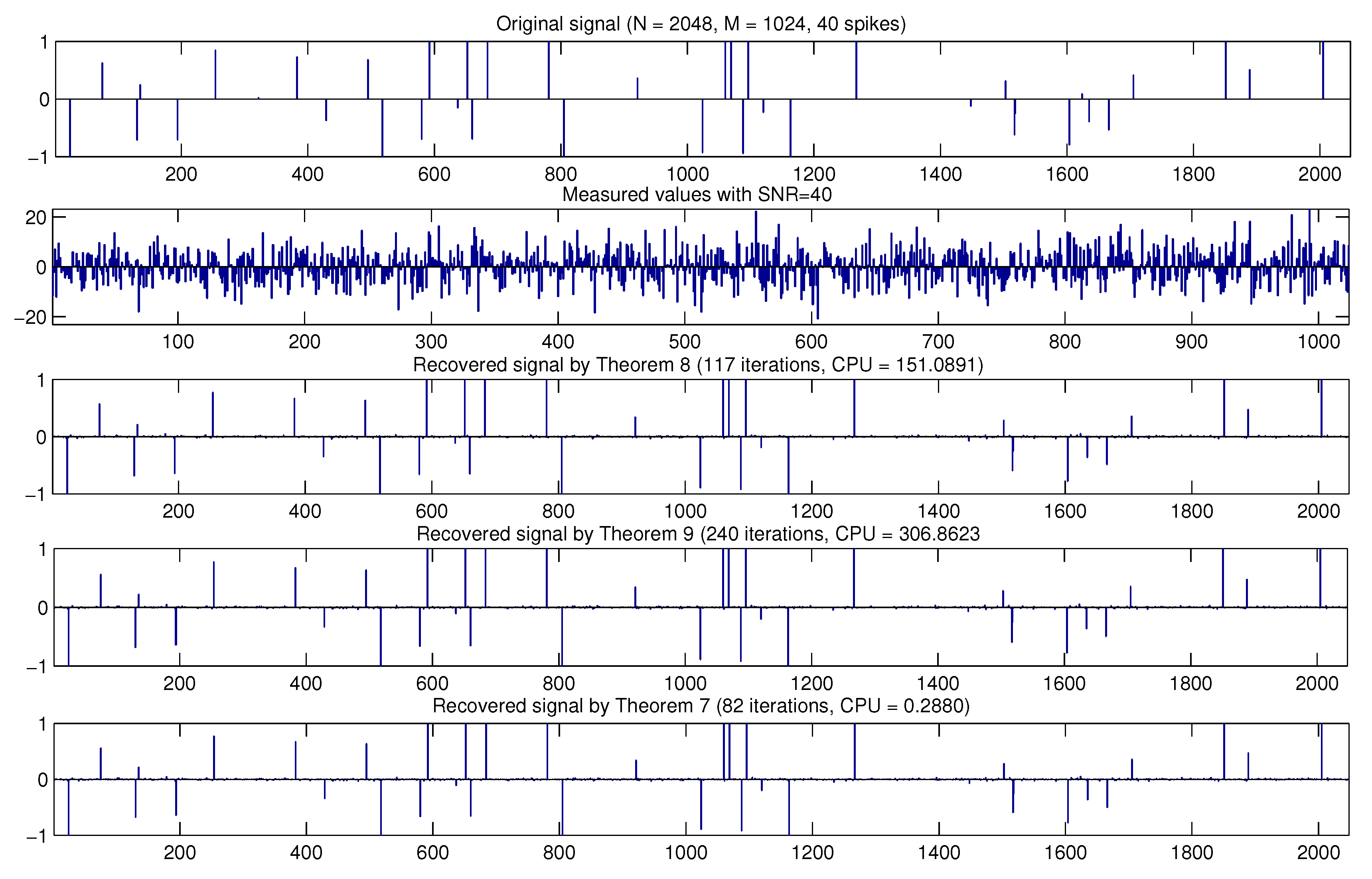
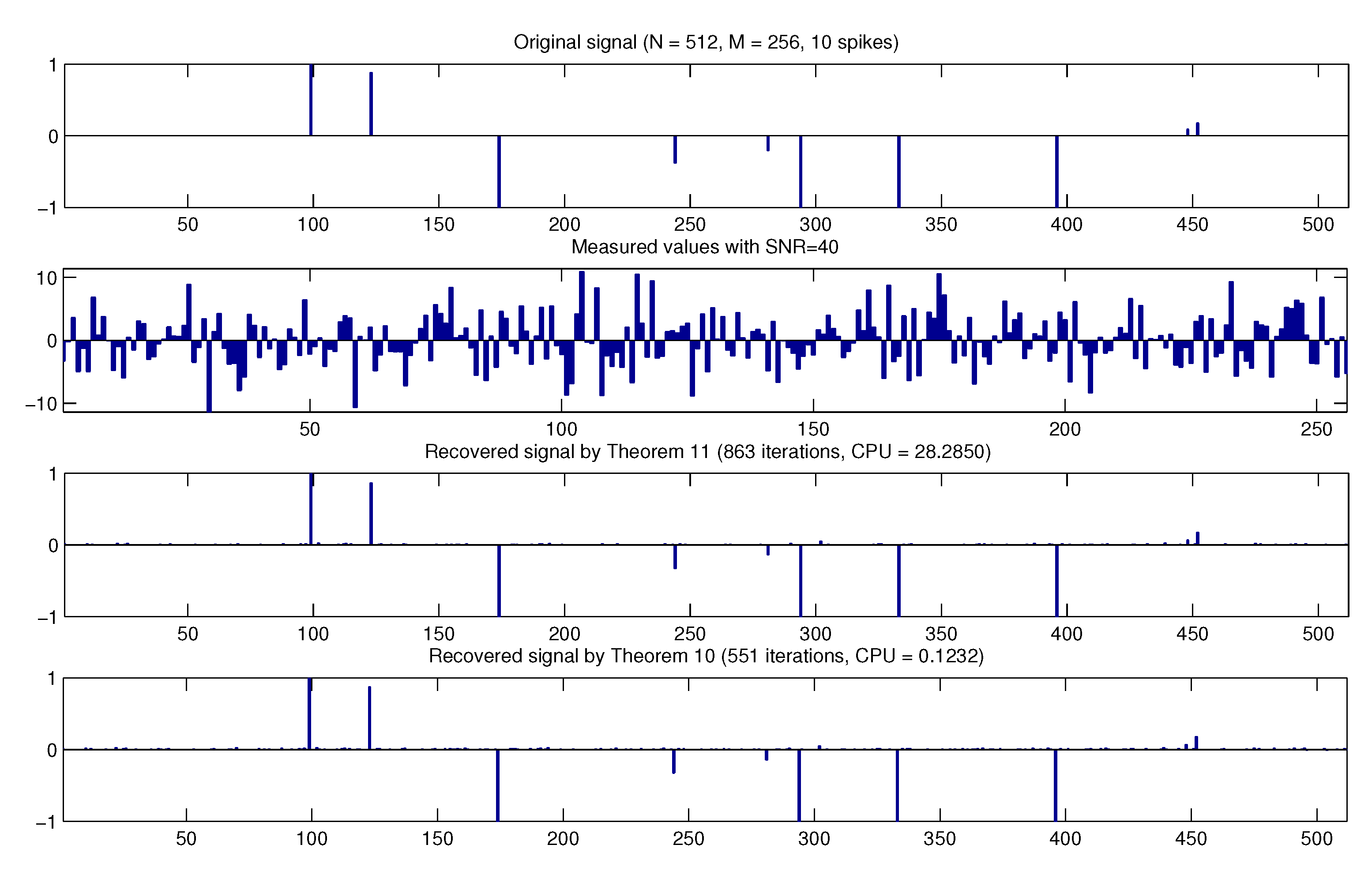
7. Applications to Compressed Sensing

In signal processing, we consider the following linear equation:

$$y=Ax+\epsilon ,$$

(73)

where $x\in {\mathbb{R}}^N$ is a sparse vector that has m nonzero components, $y\in {\mathbb{R}}^M$ is the observed data with noisy $\epsilon$, and $A:{\mathbb{R}}^N\to {\mathbb{R}}^M$$(M<N)$. It can be seen that Equation (73) relates to the LASSO problem [22]

$${\displaystyle \underset{x\in {\mathbb{R}}^N}{min}\frac{1}{2}{\parallel y-Ax\parallel }_2^2\mathrm{subject}\mathrm{to}{\parallel x\parallel }_1\le t,}$$

(74)

where $t>0$. In particular, if $C=\{x\in {\mathbb{R}}^N:\parallel x{\parallel }_1\le t\}$ and $Q=\{y\}$, then the LASSO problem can be considered as the SFP Equation (53).

The vector $x\in {\mathbb{R}}^N$ is generated by the uniform distribution in $[-2,2]$ with m nonzero components. Let A be an $M\times N$ matrix that is generated by the normal distribution with mean zero and the variance one. The observed data y is generated by white Gaussian noise with signal-to-noise ratio (SNR)40. The process is started with $t=m$ and initial point $x_1=0$.

The stopping error is defined by

$${\displaystyle E_n=\frac{1}{N}{\parallel x_n-x\parallel }_2^2<\kappa ,}$$

(75)

where $x_n$ is an estimated signal of x.

We give some numerical results of Theorems 7–9. Choose ${\gamma }_n=\frac{{\rho }_{n}f(x_n)}{\parallel g(x_n){\parallel }^2+{\theta }_n}$, ${\rho }_n=3$, ${\theta }_n=\frac{1}{n^5}$ in Theorem 7 and ${\gamma }_n=\frac{\delta }{{2\parallel A\parallel }^2}$ in Theorem 8 and $\delta =0.8$, ${\gamma }_n=\frac{\delta }{{2\parallel A\parallel }^2}$ in Theorem 9.

Table 3. Numerical results for the LASSO problem in case $M=256$, $N=512$.

m-Sparse	Method	$\mathit{\kappa }={10}^{-3}$		$\mathit{\kappa }={10}^{-4}$
		CPU	Iter	CPU	Iter
$m=10$	Theorem 8	0.9662	44	3.6208	132
	Theorem 9	1.3204	58	4.2151	170
	Theorem 7	0.0054	26	0.0111	63
$m=15$	Theorem 8	1.3082	57	2.8470	124
	Theorem 9	1.8984	84	3.7938	170
	Theorem 7	0.0058	36	0.0099	72
$m=20$	Theorem 8	1.4928	65	3.5994	161
	Theorem 9	2.7294	122	5.7801	251
	Theorem 7	0.0070	42	0.0143	99
$m=25$	Theorem 8	2.2008	98	6.0600	275
	Theorem 9	4.1730	183	18.6269	824
	Theorem 7	0.0107	67	0.0323	227

and

Table 4. Numerical results for the LASSO problem in case $M=2048$, $N=1024$.

m-Sparse	Method	$\mathit{\kappa }={10}^{-3}$		$\mathit{\kappa }={10}^{-4}$
		CPU	Iter	CPU	Iter
$m=30$	Theorem 8	47.6530	41	119.9776	101
	Theorem 9	67.6869	57	157.1087	134
	Theorem 7	0.0807	25	0.1899	58
$m=40$	Theorem 8	47.7347	41	151.0891	117
	Theorem 9	93.1898	79	306.8623	240
	Theorem 7	0.1007	31	0.2880	82
$m=50$	Theorem 8	65.1771	55	136.1508	115
	Theorem 9	99.0021	83	188.9366	158
	Theorem 7	0.1227	35	0.2203	67
$m=60$	Theorem 8	76.7457	64	163.8805	138
	Theorem 9	127.5520	106	209.5990	177
	Theorem 7	0.1401	43	0.2449	75

show that both the number of iterations and the CPU time in our algorithm in Theorem 7 are less than algorithms in Theorems 8 and 9 have in their computations. Next, we test numerical experiments in signal recovery in the case $N=512$, $M=256$ and $N=2048$, $M=1024$, respectively.

Finally, we discuss the strong convergence of Theorems 10 and 11. We set $a_n=\frac{1}{n+1}$, $b_n=\frac{1}{5}$, $c_n=1-a_n-b_n$, $d_n=0$ and ${\gamma }_n=\frac{1}{{\parallel A\parallel }^2+1}$ in Theorem 11 and set ${\rho }_n=2$, ${\theta }_n=\frac{1}{n^5}$, ${\alpha }_n=\frac{1}{n+1}$ and $u=[1,1,\dots ,1]$ in Theorem 10.

Table 5. Numerical results for the LASSO problem in case $M=512$, $N=256$.

m-Sparse	Method	$\mathit{\kappa }={10}^{-3}$		$\mathit{\kappa }={10}^{-4}$
		CPU	Iter	CPU	Iter
$m=10$	Theorem 11	5.8869	237	28.2850	863
	Theorem 10	0.0296	157	0.1232	551
$m=15$	Theorem 11	6.1204	245	38.9049	1561
	Theorem 10	0.0260	155	0.1550	950
$m=20$	Theorem 11	9.3238	376	116.7590	4613
	Theorem 10	0.0377	233	0.4484	2730
$m=25$	Theorem 11	9.3206	379	32.8208	1255
	Theorem 10	0.0420	252	0.1578	858

and

Table 6. Numerical results for the LASSO problem in case $M=2048$, $N=1024$.

m-Sparse	Method	$\mathit{\kappa }={10}^{-3}$		$\mathit{\kappa }={10}^{-4}$
		CPU	Iter	CPU	Iter
$m=10$	Theorem 11	131.3365	111	578.6894	490
	Theorem 10	0.2419	74	0.9969	305
$m=20$	Theorem 11	184.8031	157	616.7051	526
	Theorem 10	0.3274	101	1.0929	339
$m=30$	Theorem 11	262.3976	224	1.3220 × 103	503
	Theorem 10	0.4633	141	1.4516	339
$m=40$	Theorem 11	282.6013	237	1.6136 × 103	1326
	Theorem 10	0.5393	158	2.6758	791

show that our proposed algorithm in Theorem 10 has a better convergence behavior than the algorithm defined in Theorem 11 in iterations and CPU time.

We next provide some experiments in recovering the signal.

From Figure 1, Figure 2, Figure 3 and Figure 4, we observe that our algorithms can be applied to solve the LASSO problem. Moreover, the proposed algorithms have a better convergence behavior than other methods.

8. Conclusions

In the present work, we introduce a new approximation algorithm with a new stepsize that involves the self adaptive method for SVIP. The stepsize does not use the Lipschitz constant and the norm of operators in computing. We show its convergence analysis, which was proved under some suitable assumptions. The numerical results showed the efficiency of our algorithms. It is reported that the performance of our algorithms outruns those of Byrne et al. [6] and Chuang [10,11] through experiments.

References

1. Martinet, B. Régularisation d’inéquations variationnelles par approximations successives. Revue Francaise d’Informatique et de Recherche Operationelle 1970, 4, 154–158. [Google Scholar]
2. Rockafellar, R.T. Monotone operators and the proximal point algorithm. SIAM J. Control Optim. 1976, 14, 877–898. [Google Scholar] [CrossRef]
3. Moudafi, A. Split monotone variational inclusions. J. Optim. Theory Appl. 2011, 150, 275–283. [Google Scholar] [CrossRef]
4. Censor, Y.; Elfving, T. A multiprojection algorithm using Bregman projections in a product space. Numer Algor. 1994, 8, 221–239. [Google Scholar] [CrossRef]
5. Byrne, C. Iterative oblique projection onto convex sets and the split feasibility problem. Inverse Probl. 2002, 18, 441–453. [Google Scholar] [CrossRef]
6. Byrne, C.; Censor, Y.; Gibali, A. Weak and strong convergence of algorithms for the split common null point problem. J. Nonlinear Convex Anal. 2011, 13, 759–775. [Google Scholar]
7. Censor, Y.; Bortfeld, T.; Martin, B. A unified approach for inversion problems in intensity-modulated radiation therapy. Phys. Med. Biol. 2006, 51, 2353–2365. [Google Scholar] [CrossRef] [PubMed] [Green Version]
8. López, G.; Martín-Márquez, V.; Xu, H.K. Iterative algorithms for the multiple-sets split feasibility problem. In Biomedical Mathematics: Promising Directions in Imaging, Therapy Planning and Inverse Problems; Censor, Y., Jiang, M., Wang, G., Eds.; Medical Physics Publishing: Madison, WI, USA, 2010; pp. 243–279. [Google Scholar]
9. Stark, H. Image Recovery: Theory and Applications; Academic Press: San Diego, CA, USA, 1987. [Google Scholar]
10. Chuang, C.S. Algorithms with new parameter conditions for split variational inclusion problems in Hilbert spaces with application to split feasibility problem. Optimization 2016, 65, 859–876. [Google Scholar] [CrossRef]
11. Chuang, C.S. Strong convergence theorems for the split variational inclusion problem in Hilbert spaces. Fixed Point Theory Appl. 2013, 2013, 350. [Google Scholar] [CrossRef]
12. Goebel, K.; Kirk, W.A. Topics in Metric Fixed Point Theory; Cambridge Studies in Advanced Mathematics; Cambridge University Press: Cambridge, UK, 1990; Volume 28. [Google Scholar]
13. Marino, G.; Xu, H.K. Convergence of generalized proximal point algorithms. Commun. Pure Appl. Anal. 2004, 3, 791–808. [Google Scholar]
14. Opial, Z. Weak convergence of the sequence of successive approximations for nonexpansive mappings. Bull. Am. Math. Soc. 1967, 73, 591–597. [Google Scholar] [CrossRef] [Green Version]
15. He, S.; Yang, C. Solving the variational inequality problem defined on intersection of finite level sets. Abstr. Appl. Anal. 2013. [Google Scholar] [CrossRef]
16. Dang, Y.; Gao, Y. The strong convergence of a KM-CQ-like algorithm for a split feasibility problem. Inverse Prob. 2011, 27, 015007. [Google Scholar] [CrossRef]
17. Wang, F.; Xu, H.K. Approximating curve and strong convergence of the CQ algorithm for the split feasibility problem. J. Inequal. Appl. 2010, 2010, 102085. [Google Scholar] [CrossRef]
18. Xu, H.K. Iterative methods for the split feasibility problem in infinite-dimensional Hilbert spaces. Inverse Prob. 2010, 26, 105018. [Google Scholar] [CrossRef]
19. Zhao, J.; Zhang, Y.; Yang, Q. Modified projection methods for the split feasibility problem and multiple-sets feasibility problem. Appl. Math. Comput. 2012, 219, 1644–1653. [Google Scholar] [CrossRef]
20. Agarwal, R.P.; O’Regan, D.; Sahu, D.R. Fixed Point Theory for Lipschitzian-Type Mapping with Applications; Springer: New York, NY, USA, 2009; Volume 6. [Google Scholar]
21. Takahashi, W. Introduction to Nonlinear and Convex Analysis; Yokohama Tokohama Publishers, Inc.: Yokohama, Japan, 2009. [Google Scholar]
22. Tibshirani, R. Regression shrinkage and selection via the lasso. J. R. Stat. Soc. Ser. B Stat. Methodol. 1996, 58, 267–288. [Google Scholar] [CrossRef]
Figure 1. From top to bottom: original signal, measured values, recovered signal by Theorem 8, Theorem 9 and Theorem 7 with N = 512 , M = 256 and m = 10 .
Mathematics 07 00708 g001
Figure 2. From top to bottom: original signal, measured values, recovered signal by Theorem 8, Theorem 9 and Theorem 7 with N = 2048 , M = 1024 and m = 40 .
Mathematics 07 00708 g002
Figure 3. From top to bottom: original signal, measured values, recovered signal by Theorem 11 and Theorem 10 with N = 512 , M = 256 and m = 10 .
Mathematics 07 00708 g003
Figure 4. From top to bottom: original signal, measured values, recovered signal by Theorem 11 and Theorem 10 with N = 2048 , M = 1024 and m = 30 .
Mathematics 07 00708 g004