On the Solution of an Imprecisely Defined Nonlinear Time-Fractional Dynamical Model of Marriage

Abstract

The present paper investigates the numerical solution of an imprecisely defined nonlinear coupled time-fractional dynamical model of marriage (FDMM). Uncertainties are assumed to exist in the dynamical system parameters, as well as in the initial conditions that are formulated by triangular normalized fuzzy sets. The corresponding fractional dynamical system has first been converted to an interval-based fuzzy nonlinear coupled system with the help of a single-parametric gamma-cut form. Further, the double-parametric form (DPF) of fuzzy numbers has been used to handle the uncertainty. The fractional reduced differential transform method (FRDTM) has been applied to this transformed DPF system for obtaining the approximate solution of the FDMM. Validation of this method was ensured by comparing it with other methods taking the gamma-cut as being equal to one.

1. Introduction

In the present era, fractional-order derivatives have become widespread due to their wide interdisciplinary applications and implementation in various fields of science and technology, such as solid mechanics, fluid dynamics, financial mathematics, social sciences, and other areas of science and engineering (see References [1,2,3,4,5]). As the solutions of non-integer order differential equations are more complicated than integer-order differential equations, computationally efficient and reliable numerical methods need to be developed to handle these. Authors have written different books (see References [6,7,8,9,10]) in which various studies and analyses on fractional calculus may be found that will support the authors for better understanding of the concepts of fractional calculus.

The hypothesis of entropy has been connected formerly with thermodynamics only; however, in present-day, it has additionally been utilized in different areas like data hypothesis, psychodynamics, biophysical financial aspects, human relations, etc. The second law of thermodynamics expresses that entropy increases with time. It demonstrates the unpredictability of a structure over some time if there is nothing to balance out it. Likewise, in human interactions, every day, various associations lead to some turmoil. Recently, the discussion of the titled model has been attaining recognition throughout the past few years. Relational relations emerge from numerous points of view, for instance, marriage, blood relations, close attachments, work, clubs [11,12], and so forth. Many authors have studied various research related to FDMM. The nonlinear coupled fractional FDMM was first investigated by Ozalp and Koca [13]. In that paper, they performed a balance situation for equilibrium points. Khader and Alqahtani [14] applied the Bernstein collocation method for obtaining the solution of a nonlinear FDMM, and they also compared their results with the Runge–Kutta fourth-order method. They defined the fractional derivative in the Riemann–Liouville sense, and via the utilization of Bernstein polynomials, they converted the FDMM to a system of nonlinear algebraic equations, which were solved using Newton’s iterative method. Khader et al. [15] also solved the same model by implementing the Legendre spectral collocation method and affirmed the natural behavior of the present system. Singh et al. [16] implemented a q-homotopy analysis method coupled with Sumudu transform and Adomian decomposition method to solve FDMM and comparison results with the existing literature are also included. Goyal et al. [17] studied the FDMM utilizing a variation iteration method and a homotopy perturbation transform method.

Few authors have scientifically investigated the causes of extramarital interactions in marriage. It is essential and challenging to find out why some wedded couples separate, while a few couples do not. Moreover, among wedded couples, a few are fulfilled, while some are not fulfilled with each other. As such, the number of divorce cases are increasing every day all over the globe. A survey inside the U.S. uncovered that inside a forty-year interval, the probability of a first marriage finishing in separation are roughly 50 to 67 percent. The record is 10 percent higher for a second marriage. Around the world, the U.S. has the highest divorce rate. In this regard, experiments may be tough to conduct and may also be restricted for personal concerns, and so a mathematical model happens to be advantageous. As such, recently, researchers are investigating different dynamical models for interpersonal relations.

The most recent model of marriage is the Romeo and Juliet model [18]. Assume that at any moment $t$, we need to determine Romeo’s adoration or loathing for Juliet, $R\left(t\right)$ and Juliet’s affection or hate for Romeo, $J\left(t\right)$. Positive estimations of these propose love, and negative values specify hate.

The presumption about this model is that the change in Romeo’s adoration for Juliet is a small amount of his present love in addition to a small amount of her present love. Also, Juliet’s affection for Romeo will change by a small amount of her present love for Romeo and a small amount of Romeo’s adoration for her. This presumption prompts the model as given below [18,19]:

$$\begin{gathered} \frac{dR}{dt}=aR\left(t\right)+bJ\left(t\right). \\ \frac{dJ}{dt}=cR\left(t\right)+dJ\left(t\right). \end{gathered}$$

(1)

where $a,b,c$, and $d$ are constants.

Gottman et al. [20] studied the discrete dynamical model to characterize the connection between them. Since the layouts of research in those fields are cumbersome and restrained through the moral reflections, mathematical models may furthermore have a fundamental influence in considering the elements of relations and conduct highlights. A few models are present for describing the romantic relationship; however, they may be limited to integer-order differential equations.

An integer order mathematical model of love is given as follows:

$$\begin{array}{l}\frac{d\psi }{dt}=-a_1\psi +b_1\xi \left(1-\delta {\xi }^2\right)+c_1.\\ \frac{d\xi }{dt}=-a_2\xi +b_2\psi \left(1-\delta {\psi }^2\right)+c_2.\end{array}$$

(2)

Here, variables $\psi$ and $\xi$ measure the adoration of a man or woman for his/her partner. The parameters $a_i,b_i,c_i\left(1\le i\le 2\right)$ denote the oblivion, reaction, and attraction constants. We have measured that the decay of the feelings for one’s partner occurs exponentially quickly within the absence of a partner. The parameter $a_i$ indicates the degree to which one is stimulated by way of one’s personal feeling. It is used as a level of dependency along with fretfulness regarding other’s affirmation in relationships. The parameter $b_i$ represents the level to which one is supported by one’s partner and additionally anticipates him/her to be useful. It measures the tendency to keep away from or seek closeness in a relationship. The term $-a_i\psi$ and $-a_i\xi$ state that one’s adoration measure decays exponentially without one’s partner, $1/a_i$ suggests the time needed for love to diminish and $\delta$ is a compensatory constant.

In the present study, a time-fractional order dynamical system has been considered instead of its integer order system because fractional order equations are generalizations of integer order differential equations and fractional order models hold memory. Interpersonal relationships are influenced by memory, which makes the modeling more appropriate than the integer one for this kind of dynamical system. This fact confirms that fractional modeling is best suited for this kind of system. Hence, the investigation of the time-fractional systems is significant. The FDMM is given as:

$$\begin{array}{l}\frac{d^{\alpha }\psi }{d{t}^{\alpha }}=-a_1\psi +b_1\xi \left(1-\delta {\xi }^2\right)+c_1.\\ \frac{d^{\alpha }\xi }{d{t}^{\alpha }}=-a_2\xi +b_2\psi \left(1-\delta {\psi }^2\right)+c_2.\end{array}$$

(3)

$$\mathrm{where} 0<\alpha \le 1 a_i\ge 0$$

with initial conditions (ICs):

$$\psi \left(0\right)=0=\xi \left(0\right)$$

(4)

It is observed that all the authors mentioned above have considered the parameters and variables involved in FDMM as crisp or precise. However, in real life, it may not always be possible to take crisp values due to errors in experiments, observations, and many other errors. Therefore, the parameters and variables may be considered as uncertain. Here, the uncertainties are considered as intervals/fuzzy. The parameters $a_i,b_i,c_i\left(1\le i\le 2\right)$ and $\delta$ denote the oblivion, reaction, attraction, and compensatory constants, respectively. As these parameters are related to attractions and reactions of the model, its values may not always be fixed. As such, the main targets of the authors are to consider these parameters as fuzzy and then solve this fuzzy fractional model using an efficient method.

Let us consider the coupled fuzzy FDMM as given below:

$$\begin{array}{l}\frac{d^{\alpha }\tilde{\psi }}{d{t}^{\alpha }}=-\left(a_1-0.02,a_1,a_1+0.02\right)\tilde{\psi }+\left(b_1-0.02,b_1,b_1+0.02\right)\tilde{\xi }\\ \left\{1-\left(\delta -0.01,\delta ,\delta +0.01\right){\tilde{\xi }}^2\right\}+\left(c_1-0.2,c_1,c_1+0.2\right).\\ \frac{d^{\alpha }\tilde{\xi }}{d{t}^{\alpha }}=-\left(a_2-0.02,a_2,a_2+0.02\right)\tilde{\xi }+\left(b_2-0.02,b_2,b_2+0.02\right)\tilde{\psi }\\ \left\{1-\left(\delta -0.01,\delta ,\delta +0.01\right){\tilde{\psi }}^2\right\}+\left(c_2-0.2,c_2,c_2+0.2\right).\end{array}$$

(5)

with fuzzy ICs

$$\tilde{\psi }\left(0\right)=\tilde{\xi }\left(0\right)=\left(-0.1,0,0.1\right)$$

(6)

where variables $\tilde{\psi }$ and $\tilde{\xi }$ describe the uncertain adoration of a man or woman for his/her partner.

The basic concepts of fuzzy variables were first presented by Chang and Zadeh [21], where they suggested the theory of a fuzzy derivative. The extensive analysis in Chang and Zadeh [21] was well-defined and studied by Dubois and Prade [22]. Kaleva [23] and Seikkala [24] studied the fuzzy differential equations (FDEs) and initial value problems. Various problems related to the differential FDEs are broadly studied by Chakraverty et al. (see References [25,26,27]). As fuzzy fractional differential equations (FFDEs) are quite challenging to solve as compared to fractional differential equations, computationally efficient numerical methods should be developed. In this research, we have applied a fractional reduced differential transform method (FRDTM) along with imprecisely defined parameters involved in the FDMM in order to study this dynamical system. Also, the convergence analysis of the present solution has been discussed with an increasing number of terms of the solution. The double-parametric form of a fuzzy number is applied to find the solution of the fractional fuzzy dynamical model of marriage. This model has not yet been studied using FRDTM. The main benefit of using this technique are: First, this procedure achieves the expansions of the solutions. Second, this technique does not require any discretization, perturbations, or modification of the ICs. Also, this technique needs fewer computations with high precision, as well as less time compared to other techniques. In view of the above literature, FFDEs are first changed to a differential equation using a double-parametric form (DPF). Then, the equivalent equation is solved using FRDTM to have an interval/fuzzy solution in terms of the DPF.

The remaining parts of the manuscript are arranged as follows. In the “Preliminaries” section, we give essential information related to fuzzy arithmetic, triangular fuzzy number, and double-parametric form of a fuzzy number. In section “Fractional Reduced Differential Transform Method,” we discuss methodology and important theorems related to this technique. The double-parametric form-based solution of FDMM is given in section “Double-Parametric-Based Solution of Uncertainty FDMM Using FRDTM.” Next, numerical outcomes and deliberations are given in the “Results and Discussions” section. Finally, conclusions are drawn.

2. Preliminaries

In this segment, some basic definitions, and notations of fuzzy variables are discussed (see References [25,26,27]).

Definition 1. (Fuzzy Number)

A fuzzy number$\tilde{\psi }$is a convex normalized fuzzy set$\tilde{\psi }$of the real line$\Re$such that:

$$\left\{{\mu }_{\tilde{\psi }}\left(x\right):\Re \to [0,1],\forall x\in \Re \right\}$$

where${\mu }_{\tilde{\psi }}$is a membership function and is piecewise continuous.

Definition 2. (Triangular Fuzzy Number)

A triangular fuzzy number$\tilde{\psi }$is a convex normalized fuzzy set$\tilde{\psi }$of the real line$\Re$such that:

(a) 

There exists exactly one$x_0\in \Re$with${\mu }_{\tilde{\psi }}\left(x_0\right)$($x_0$is called the mean value of$\tilde{\psi }$), where${\mu }_{\tilde{\psi }}$is called the membership function of the fuzzy set.

(b) 

${\mu }_{\tilde{\psi }}\left(x\right)$is piecewise continuous.

The membership function${\mu }_{\tilde{\psi }}$of a triangular fuzzy number$\tilde{\psi }=\left(a_1,b_1,c_1\right)$is defined as:

$${\mu }_{\tilde{\psi }}\left(x\right)=\{\begin{array}{ll}0,& x\le a_1,\\ \frac{x-a_1}{b_1-a_1},& a_1\le x\le b_1,\\ \frac{c_1-x}{c_1-b_1},& b_1\le x\le c_1,\\ 0,& x\ge c_1.\end{array}$$

Definition 3. (Single-Parametric Form of Fuzzy Numbers)

The triangular fuzzy number$\tilde{\psi }=\left(a_1,b_1,c_1\right)$can be characterized by an ordered pair of functions through the$\gamma$-cut approach$\lfloor \underset{\_}{\psi }\left(\gamma \right),\overline{\psi }\left(\gamma \right)\rfloor =[\left(b_1-a_1\right)\gamma +a_1,-\left(c_1-b_1\right)\gamma +c_1]$, where$\gamma \in [0,1]$. The$\gamma$-cut form is well-known as the single-parametric form of fuzzy numbers. It is observed that the lower and upper bounds of the fuzzy numbers satisfy the below statements:

(i) 

$\underset{\_}{\psi }\left(\gamma \right)$is a left-bounded nondecreasing continuous function over$[0,1]$.

(ii) 

$\overline{\psi }\left(\gamma \right)$is a right-bounded nonincreasing continuous function over$[0,1]$.

(iii) 

$\underset{\_}{\psi }\left(\gamma \right)\le \overline{\psi }\left(\gamma \right)$, where$0\le \gamma \le 1.$

Definition 4. (Double-Parametric Form of Fuzzy Number)

Using the single-parametric form, as discussed in Definition 3, we have$\tilde{\psi }=[\underset{\_}{\psi }\left(\gamma \right),\overline{\psi }\left(\gamma \right)]$.

Now we can write this as crisp with DPF as:

$$\tilde{\psi }\left(\gamma ,\beta \right)=\beta \left(\overline{\psi }\left(\gamma \right)-\underset{\_}{\psi }\left(\gamma \right)\right)+\underset{\_}{\psi }\left(\gamma \right)$$

where$\gamma$and$\beta \in [0,1]$.

Definition 5. (Fuzzy Arithmetic)

For arbitrary fuzzy numbers$\tilde{x}=\lfloor \underset{\_}{x}\left(\gamma \right),\overline{x}\left(\gamma \right)\rfloor$,$\tilde{y}=\lfloor \underset{\_}{y}\left(\gamma \right),\overline{y}\left(\gamma \right)\rfloor$and scalar$m$, fuzzy arithmetics are well-defined as below:

(i) 

$\tilde{x}=\tilde{y}$if and only if$\underset{\_}{x}\left(\gamma \right)=\underset{\_}{y}\left(\gamma \right)$and$\overline{x}\left(\gamma \right)=\overline{y}\left(\gamma \right)$.

(ii) 

$\tilde{x}+\tilde{y}=\lfloor \underset{\_}{x}\left(\gamma \right)+\underset{\_}{y}\left(\gamma \right),\overline{x}\left(\gamma \right)+\overline{y}\left(\gamma \right)\rfloor$.

(iii) 

$\tilde{x}\times \tilde{y}=\left[\begin{array}{l}\min \left(\underset{\_}{x}\left(\gamma \right)\times \underset{\_}{y}\left(\gamma \right),\underset{\_}{x}\left(\gamma \right)\times \overline{y}\left(\gamma \right),\overline{x}\left(\gamma \right)\times \underset{\_}{y}\left(\gamma \right),\overline{x}\left(\gamma \right)\times \overline{y}\left(\gamma \right)\right),\\ \max \left(\underset{\_}{x}\left(\gamma \right)\times \underset{\_}{y}\left(\gamma \right),\underset{\_}{x}\left(\gamma \right)\times \overline{y}\left(\gamma \right),\overline{x}\left(\gamma \right)\times \underset{\_}{y}\left(\gamma \right),\overline{x}\left(\gamma \right)\times \overline{y}\left(\gamma \right)\right)\end{array}\right]$.

(iv) 

$k\tilde{x}=\{\begin{array}{l}[k\overline{x}\left(\gamma \right),k\underset{\_}{x}\left(\gamma \right)],k<0\\ [k\underset{\_}{x}\left(\gamma \right),k\overline{x}\left(\gamma \right)],k\ge 0\end{array}.$

3. Fractional Reduced Differential Transform Method

Let us take an analytic and k-times continuously differentiable function $\psi \left(x,t\right)$. Assume that $\psi \left(x,t\right)$ is denoted as a product of two functions as $\psi \left(x,t\right)=a\left(x\right)b\left(t\right)$. From Momani and Odibat [28], this function is written as follows

$$\psi \left(x,t\right)=\left({\displaystyle \sum _{m=0}^{\infty }A\left(m\right)}{x}^m\right)\left({\displaystyle \sum _{n=0}^{\infty }B\left(n\right)}{t}^n\right)={\displaystyle \sum _{m=0}^{\infty }{\displaystyle \sum _{n=0}^{\infty }F\left(m,n\right)}{x}^m}{t}^n$$

(7)

where $F\left(m,n\right)=A\left(m\right)B\left(n\right)$ is named as the spectrum of $\psi \left(x,t\right)$.

Lemma 1.

The fractional reduced differential transform (FRDT) of an analytic function$\psi \left(x,t\right)$is defined as:

$${\psi }_k\left(x\right)=\frac{1}{\mathsf{\Gamma }\left(1+\alpha k\right)}{[D_t^{\alpha k}\psi \left(x,t\right)]}_{t=t_0}\mathrm{for}k=0,1,2,\dots$$

(8)

The inverse transform of${\psi }_k\left(x\right)$is well-defined as

$$\psi \left(x,t\right)={\displaystyle \sum _{k=0}^{\infty }{\psi }_k\left(x\right){\left(t-t_0\right)}^{\alpha k}}$$

(9)

From Equations (8) and (9), we obtain:

$$\psi \left(x,t\right)={\displaystyle \sum _{k=0}^{\infty }\frac{1}{\mathsf{\Gamma }\left(\alpha k+1\right)}}{[D_t^{\alpha k}\psi \left(x,t\right)]}_{t=t_0}{\left(t-t_0\right)}^{\alpha k}$$

(10)

In particular, at$t_0=0$, we have:

$$\psi \left(x,t\right)={\displaystyle \sum _{k=0}^{\infty }\frac{1}{\mathsf{\Gamma }\left(\alpha k+1\right)}}{[D_t^{\alpha k}\psi \left(x,t\right)]}_{t=0}{t}^{\alpha k}$$

(11)

Theorem 1.

Let$\psi \left(x,t\right),\xi \left(x,t\right)$, and$\zeta \left(x,t\right)$be three analytical functions such that$\psi \left(x,t\right)=R_D^{-1}[{\psi }_k\left(x\right)]$,$\xi \left(x,t\right)=R_D^{-1}[{\xi }_k\left(x\right)]$, and$\zeta \left(x,t\right)=R_D^{-1}[{\zeta }_k\left(x\right)]$. Hence from References [29,30,31,32]):

(i) 

If$\psi \left(x,t\right)=c_1\xi \left(x,t\right)\pm c_2\zeta (x,t)$, then${\psi }_k\left(x\right)=c_1{\xi }_k\left(x\right)\pm c_2{\zeta }_k(x)$, where$c_1$and$c_2$are constants.

(ii) 

If$\psi \left(x,t\right)=a\xi \left(x,t\right)$, then${\psi }_k\left(x\right)=a{\xi }_k\left(x\right)$.

(iii) 

If$\psi \left(x,t\right)=x^m{t}^n$, then${\psi }_k\left(x\right)=x^m\delta \left(k-n\right)$where$\delta \left(k\right)=\{\begin{array}{l}1,k=0\\ 0,k\ne 0\end{array}$.

(iv) 

If$\psi \left(x,t\right)=x^m{t}^n\xi \left(x,t\right)$, then${\psi }_k\left(x\right)=x^m{\xi }_{k-n}\left(x\right)$.

(v) 

If$\psi \left(x,t\right)=\xi \left(x,t\right)\zeta (x,t)$, then${\psi }_k\left(x\right)={\displaystyle \sum _{i=0}^j{\xi }_i}\left(x\right){\zeta }_{j-i}(x)={\displaystyle \sum _{i=0}^j{\zeta }_i}\left(x\right){\xi }_{j-i}(x)$.

(vi) 

If$\psi \left(x,t\right)=\xi \left(x,t\right)\zeta (x,t)\varsigma (x,t)$, then${\psi }_k\left(x\right)={\displaystyle \sum _{j=0}^k{\displaystyle \sum _{i=0}^j{\xi }_i}\left(x\right){\zeta }_{j-i}(x)}{\varsigma }_{k-j}(x)$.

Theorem 2.

Let$\psi \left(x,t\right)$and$\xi \left(x,t\right)$are two analytical functions such that$\psi \left(x,t\right)=R_D^{-1}[{\psi }_k\left(x\right)]$, and$\xi \left(x,t\right)=R_D^{-1}[{\xi }_k\left(x\right)]$. Hence:

(i) 

If$\psi \left(x,t\right)=\frac{{\partial }^m}{\partial x^m}\xi \left(x,t\right)$,then${\psi }_k\left(x\right)=\frac{{\partial }^m}{\partial x^m}{\xi }_k\left(x\right)$.

(ii) 

If$\psi \left(x,t\right)=\frac{{\partial }^{n\alpha }}{\partial t^{n\alpha }}\xi \left(x,t\right)$, then${\psi }_k\left(x\right)=\frac{\mathsf{\Gamma }\left(1+\left(k+n\right)\alpha \right)}{\left(1+k\alpha \right)}{\xi }_{k+n}\left(x\right)$.

Corollary 1.

If$\zeta \left(x,t\right)=e^{\delta t+\theta x}$, then${\zeta }_k\left(x\right)=\frac{{\delta }^k}{k!}{e}^{\theta x}$.

Corollary 2.

If$\xi \left(x,t\right)=\sin (\theta t+\mu x)$and$\zeta \left(x,t\right)=\cos (\theta t+\mu x)$, then${\xi }_k\left(x\right)=\frac{{\theta }^k}{k!}\sin \left(\frac{k\pi }{2}+\mu x\right)$and${\zeta }_k\left(x\right)=\frac{{\theta }^k}{k!}\cos \left(\frac{k\pi }{2}+\mu x\right)$.

In order to explain the concept of FRDTM, let us consider the following equation in the operator form as:

$$L\psi \left(x,t\right)+R\psi \left(x,t\right)+N\psi \left(x,t\right)=h\left(x,t\right)$$

(12)

with IC:

$$\psi \left(x,0\right)=g\left(x\right)$$

(13)

where $L=\frac{{\partial }^{\alpha }}{\partial t^{\alpha }}$; $R$, $N$ are linear, nonlinear operators; and $h\left(x,t\right)$ is an inhomogeneous source term.

Using Theorem 2 and Equations (8) and (12), this reduces to:

$$\frac{\mathsf{\Gamma }\left(1+\alpha k+\alpha \right)}{\mathsf{\Gamma }\left(1+\alpha k\right)}{\psi }_{k+1}\left(x\right)=H_k\left(x\right)-R{\psi }_k\left(x\right)-N{\psi }_k\left(x\right)\mathrm{for}k=0,1,2\dots$$

(14)

where ${\psi }_k\left(x\right)$ and $H_k\left(x\right)$ are the transformed form of $\psi \left(x,t\right)$ and $h\left(x,t\right)$, respectively.

Applying FRDTM on the IC, we obtain:

$${\psi }_0\left(x\right)=g\left(x\right)$$

(15)

Using Equations (14) and (15), ${\psi }_k(x)$ for $k=1,2,3,\dots$ can be determined.

Then, taking the inverse transformation of ${\left\{{\psi }_k\left(x\right)\right\}}_{k=0}^n$ gives the n-term approximate solution as:

$${\psi }_n\left(x,t\right)={\displaystyle \sum _{k=0}^n{\psi }_k\left(x\right)t^{\alpha k}}$$

(16)

Therefore, the analytical result of Equation (12) is written as $\psi \left(x,t\right)=\underset{n\to \infty }{\lim }{\psi }_n\left(x,t\right)$.

4. Double-Parametric-Based Solution of an Uncertain FDMM Using FRDTM

To begin with, by applying the single parametric form, the FDMM is changed to an interval-based FDE. At that moment, by applying the DPF, the interval-based FDE is transformed into an FDMM having two parameters that may control the uncertainty. Finally, FRDTM is then applied to solve the corresponding double parametrized FDMM for obtaining the needed solution in terms of intervals/fuzzy variables.

Equations (5) and (6) can now be modified in single-parametric form as:

$$\begin{array}{r}\left[\frac{d^{\alpha }}{d{t}^{\alpha }}\underset{\_}{\psi }\left(t;\gamma \right),\frac{d^{\alpha }}{d{t}^{\alpha }}\overline{\psi }\left(t;\gamma \right)\right]=-\left[\left(0.02\gamma +a_1-0.02\right),(-0.02\gamma +a_1+0.02)\right]\left[\underset{\_}{\psi }\left(t;\gamma \right),\overline{\psi }\left(t;\gamma \right)\right]\\ +\left[\left(0.02\gamma +b_1-0.02\right),(-0.02\gamma +b_1+0.02)\right]\left[\underset{\_}{\xi }\left(t;\gamma \right),\overline{\xi }\left(t;\gamma \right)\right]\\ \left[1-\left\{\left(0.01\gamma +\delta -0.01\right),(-0.01\gamma +\delta +0.01)\right\}{\left\{\underset{\_}{\xi }\left(t;\gamma \right),\overline{\xi }\left(t;\gamma \right)\right\}}^2\right]\\ +\left[\left(0.2\gamma +c_1-0.2\right),(-0.2\gamma +c_1+0.2)\right]\\ \left[\frac{d^{\alpha }}{d{t}^{\alpha }}\underset{\_}{\xi }\left(t;\gamma \right),\frac{d^{\alpha }}{d{t}^{\alpha }}\overline{\xi }\left(t;\gamma \right)\right]=-\left[\left(0.02\gamma +a_2-0.02\right),(-0.02\gamma +a_2+0.02)\right]\left[\underset{\_}{\xi }\left(t;\gamma \right),\overline{\xi }\left(t;\gamma \right)\right]\\ +\left[\left(0.02\gamma +b_2-0.02\right),(-0.02\gamma +b_2+0.02)\right]\left[\underset{\_}{\psi }\left(t;\gamma \right),\overline{\psi }\left(t;\gamma \right)\right]\\ \left[1-\left\{\left(0.01\gamma +\delta -0.01\right),(-0.01\gamma +\delta +0.01)\right\}{\left\{\underset{\_}{\psi }\left(t;\gamma \right),\overline{\psi }\left(t;\gamma \right)\right\}}^2\right]\\ +\left[\left(0.2\gamma +c_2-0.2\right),(-0.2\gamma +c_2+0.2)\right].\end{array}$$

(17)

with fuzzy ICs:

$$\left[\underset{\_}{\psi }\left(0;\gamma \right),\overline{\psi }\left(0;\gamma \right)\right]=\left[\underset{\_}{\xi }\left(0;\gamma \right),\overline{\xi }\left(0;\gamma \right)\right]=\left[0.1\gamma -0.1,-0.1\gamma +0.1\right]$$

(18)

where Equations (17) and (18) are in interval form. One can find out the solution of this interval equations, but sometimes it is complicated to handle such types of interval equations. Therefore, one may require the double-parametric form to handle this interval computation. Applying double-parametric form to Equations (17) and (18), we have:

$$\begin{array}{l}\left\{\beta \left(\frac{d^{\alpha }}{d{t}^{\alpha }}\overline{\psi }\left(t;\gamma \right)-\frac{d^{\alpha }}{d{t}^{\alpha }}\underset{\_}{\psi }\left(t;\gamma \right)\right)+\frac{d^{\alpha }}{d{t}^{\alpha }}\underset{\_}{\psi }\left(t;\gamma \right)\right\}=\left\{\beta \left(0.04-0.04\gamma \right)+0.02\gamma -0.02+a_1\right\}\\ \left\{\beta \left(\overline{\psi }\left(t;\gamma \right)-\underset{\_}{\psi }\left(t;\gamma \right)\right)+\underset{\_}{\psi }\left(t;\gamma \right)\right\}+\left\{\beta \left(0.04-0.04\gamma \right)+0.02\gamma +b_1-0.02\right\}\\ \left\{\beta \left(\overline{\xi }\left(t;\gamma \right)-\underset{\_}{\xi }\left(t;\gamma \right)\right)+\underset{\_}{\xi }\left(t;\gamma \right)\right\}\left[\begin{array}{l}1-\left\{\beta \left(0.02-0.02\gamma \right)+0.01\gamma +\delta -0.01\right\}\\ {\left\{\beta \left(\overline{\xi }\left(t;\gamma \right)-\underset{\_}{\xi }\left(t;\gamma \right)\right)+\underset{\_}{\xi }\left(t;\gamma \right)\right\}}^2\end{array}\right]\\ +\left\{\beta \left(0.4-0.4\gamma \right)+0.2\gamma +c_1-0.2\right\}.\end{array}$$

(19)

$$\begin{array}{l}\left\{\beta \left(\frac{d^{\alpha }}{d{t}^{\alpha }}\overline{\xi }\left(t;\gamma \right)-\frac{d^{\alpha }}{d{t}^{\alpha }}\underset{\_}{\xi }\left(t;\gamma \right)\right)+\frac{d^{\alpha }}{d{t}^{\alpha }}\underset{\_}{\xi }\left(t;\gamma \right)\right\}=\left\{\beta \left(0.04-0.04\gamma \right)+0.02\gamma -0.02+a_2\right\}\\ \left\{\beta \left(\overline{\xi }\left(t;\gamma \right)-\underset{\_}{\xi }\left(t;\gamma \right)\right)+\underset{\_}{\xi }\left(t;\gamma \right)\right\}+\left\{\beta \left(0.04-0.04\gamma \right)+0.02\gamma +b_2-0.02\right\}\\ \left\{\beta \left(\overline{\psi }\left(t;\gamma \right)-\underset{\_}{\psi }\left(t;\gamma \right)\right)+\underset{\_}{\psi }\left(t;\gamma \right)\right\}\left[\begin{array}{l}1-\left\{\beta \left(0.02-0.02\gamma \right)+0.01\gamma +\delta -0.01\right\}\\ {\left\{\beta \left(\overline{\psi }\left(t;\gamma \right)-\underset{\_}{\psi }\left(t;\gamma \right)\right)+\underset{\_}{\psi }\left(t;\gamma \right)\right\}}^2\end{array}\right]\\ +\left\{\beta \left(0.4-0.4\gamma \right)+0.2\gamma +c_2-0.2\right\}.\end{array}$$

(20)

with fuzzy ICs:

$$\begin{array}{l}\left\{\beta \left(\overline{\psi }\left(0;\gamma \right)-\underset{\_}{\psi }\left(0;\gamma \right)\right)+\underset{\_}{\psi }\left(0;\gamma \right)\right\}=\left\{\beta \left(\overline{\xi }\left(0;\gamma \right)-\underset{\_}{\xi }\left(0;\gamma \right)\right)+\underset{\_}{\xi }\left(0;\gamma \right)\right\}\\ =\beta \left(-0.2\gamma +0.2\right)+\left(0.1\gamma -0.1\right)\end{array}$$

(21)

Let us take:

$$\begin{gathered} \left\{\beta \left(\frac{d^{\alpha }}{d{t}^{\alpha }}\overline{\xi }\left(t;\gamma \right)-\frac{d^{\alpha }}{d{t}^{\alpha }}\underset{\_}{\xi }\left(t;\gamma \right)\right)+\frac{d^{\alpha }}{d{t}^{\alpha }}\underset{\_}{\xi }\left(t;\gamma \right)\right\}=\frac{d^{\alpha }}{d{t}^{\alpha }}\tilde{\xi }\left(t;\gamma ,\beta \right) \\ \left\{\beta \left(\frac{d^{\alpha }}{d{t}^{\alpha }}\overline{\psi }\left(t;\gamma \right)-\frac{d^{\alpha }}{d{t}^{\alpha }}\underset{\_}{\psi }\left(t;\gamma \right)\right)+\frac{d^{\alpha }}{d{t}^{\alpha }}\underset{\_}{\psi }\left(t;\gamma \right)\right\}=\frac{d^{\alpha }}{d{t}^{\alpha }}\tilde{\psi }\left(t;\gamma ,\beta \right) \\ \left\{\beta \left(\overline{\psi }\left(t;\gamma \right)-\underset{\_}{\psi }\left(t;\gamma \right)\right)+\underset{\_}{\psi }\left(t;\gamma \right)\right\}=\tilde{\psi }\left(t;\gamma ,\beta \right) \\ \left\{\beta \left(\overline{\xi }\left(t;\gamma \right)-\underset{\_}{\xi }\left(t;\gamma \right)\right)+\underset{\_}{\xi }\left(t;\gamma \right)\right\}=\tilde{\xi }\left(t;\gamma ,\beta \right). \\ \left\{\beta \left(0.04-0.04\gamma \right)+0.02\gamma -0.02+a_1\right\}={\tilde{a}}_1. \\ \left\{\beta \left(0.04-0.04\gamma \right)+0.02\gamma -0.02+a_2\right\}={\tilde{a}}_2. \\ \left\{\beta \left(0.04-0.04\gamma \right)+0.02\gamma +b_1-0.02\right\}={\tilde{b}}_1. \\ \left\{\beta \left(0.04-0.04\gamma \right)+0.02\gamma +b_2-0.02\right\}={\tilde{b}}_2. \\ \left\{\beta \left(0.4-0.4\gamma \right)+0.2\gamma +c_1-0.2\right\}={\tilde{c}}_1. \\ \left\{\beta \left(0.4-0.4\gamma \right)+0.2\gamma +c_2-0.2\right\}={\tilde{c}}_2. \\ \left\{\beta \left(0.02-0.02\gamma \right)+0.01\gamma +\delta -0.01\right\}=\tilde{\delta }. \\ \left\{\beta \left(\overline{\psi }\left(0;\gamma \right)-\underset{\_}{\psi }\left(0;\gamma \right)\right)+\underset{\_}{\psi }\left(0;\gamma \right)\right\}=\tilde{\psi }\left(0;\gamma ,\beta \right) \end{gathered}$$

and

$$\left\{\beta \left(\overline{\xi }\left(0;\gamma \right)-\underset{\_}{\xi }\left(0;\gamma \right)\right)+\underset{\_}{\xi }\left(0;\gamma \right)\right\}=\tilde{\xi }\left(0;\gamma ,\beta \right)$$

Substituting all the above equations in Equations (19)–(21), we get:

$$\begin{array}{l}\frac{d^{\alpha }\tilde{\psi }\left(t;\gamma ,\beta \right)}{d{t}^{\alpha }}=-{\tilde{a}}_1\tilde{\psi }\left(t;\gamma ,\beta \right)+{\tilde{b}}_1\tilde{\xi }\left(t;\gamma ,\beta \right)\left(1-\tilde{\delta }{\tilde{\xi }}^2\left(t;\gamma ,\beta \right)\right)+{\tilde{c}}_1.\\ \frac{d^{\alpha }\tilde{\xi }\left(t;\gamma ,\beta \right)}{d{t}^{\alpha }}=-{\tilde{a}}_2\tilde{\xi }\left(t;\gamma ,\beta \right)+{\tilde{b}}_2\tilde{\psi }\left(t;\gamma ,\beta \right)\left(1-\tilde{\delta }{\tilde{\psi }}^2\left(t;\gamma ,\beta \right)\right)+{\tilde{c}}_2.\end{array}$$

(22)

with ICs:

$$\tilde{\psi }\left(0;\gamma ,\beta \right)=\tilde{\xi }\left(0;\gamma ,\beta \right)=\beta \left(-0.2\gamma +0.2\right)+\left(0.1\gamma -0.1\right)=\eta$$

(23)

Solving Equation (22) with the ICs in Equation (23), we have ${\tilde{\psi }}_1\left(t;\gamma ,\beta \right)$ and ${\tilde{\psi }}_2\left(t;\gamma ,\beta \right)$ in terms of $\gamma$ and $\beta$. To find the lower and upper bounds of the solutions in single parametric form, we have to substitute $\beta =0$ and $\beta =1$, respectively. Mathematically these are written as:

$$\tilde{\psi }\left(t;\gamma ,0\right)=\underset{\_}{\psi }\left(t;\gamma \right),\tilde{\xi }\left(t;\gamma ,0\right)=\underset{\_}{\xi }\left(t;\gamma \right)\mathrm{and}\tilde{\psi }\left(t;\gamma ,1\right)=\overline{\psi }\left(t;\gamma \right),\tilde{\xi }\left(t;\gamma ,1\right)=\overline{\xi }\left(t;\gamma \right)$$

Applying FRDTM to both sides of Equation (22), and using Theorems 1 and 2, we have:

$$\begin{array}{l}\frac{\mathsf{\Gamma }\left(1+k\alpha +\alpha \right)}{\mathsf{\Gamma }\left(1+k\alpha \right)}{\tilde{\psi }}_{k+1}\left(\gamma ,\beta \right)=-{\tilde{a}}_1{\tilde{\psi }}_k\left(\gamma ,\beta \right)+{\tilde{b}}_1{\tilde{\xi }}_k\left(\gamma ,\beta \right)-{\tilde{b}}_1\tilde{\delta }\left({\displaystyle \sum _{i=0}^k{\displaystyle \sum _{j=0}^i{\tilde{\xi }}_{i-j}{\tilde{\xi }}_j{\tilde{\xi }}_{k-i}}}\right)+{\tilde{c}}_1\delta \left(k\right)\\ \frac{\mathsf{\Gamma }\left(1+k\alpha +\alpha \right)}{\mathsf{\Gamma }\left(1+k\alpha \right)}{\tilde{\xi }}_{k+1}\left(\gamma ,\beta \right)=-{\tilde{a}}_2{\tilde{\xi }}_k\left(\gamma ,\beta \right)+{\tilde{b}}_2{\tilde{\psi }}_k\left(\gamma ,\beta \right)-{\tilde{b}}_2\tilde{\delta }\left({\displaystyle \sum _{i=0}^k{\displaystyle \sum _{j=0}^i{\tilde{\psi }}_{i-j}{\tilde{\psi }}_j{\tilde{\psi }}_{k-i}}}\right)+{\tilde{c}}_2\delta \left(k\right)\end{array}$$

(24)

Where:

$$\delta \left(k\right)=\{\begin{array}{ll}1,& k=0\\ 0,& k\ne 0\end{array}$$

Using FRDTM on the IC, we get:

$${\tilde{\psi }}_0\left(\gamma ,\beta \right)={\tilde{\xi }}_0\left(\gamma ,\beta \right)=\eta$$

(25)

Using Equation (25) in Equation (24), the following values of ${\tilde{\psi }}_k$ and ${\tilde{\xi }}_k$ for $k=1,2,\dots$ are obtained:

$$\begin{array}{l}{\tilde{\psi }}_1=-{\tilde{a}}_1\eta +{\tilde{b}}_1\eta -{\tilde{b}}_1\tilde{\delta }{\eta }^3+{\tilde{c}}_1.\\ {\tilde{\xi }}_1=-{\tilde{a}}_2\eta +{\tilde{b}}_2\eta -{\tilde{b}}_2\tilde{\delta }{\eta }^3+{\tilde{c}}_2.\end{array}$$

(26)

$$\begin{array}{l}{\tilde{\psi }}_2=-{\tilde{a}}_1\left(-{\tilde{a}}_1\eta +{\tilde{b}}_1\eta -{\tilde{b}}_1\tilde{\delta }{\eta }^3+{\tilde{c}}_1\right)+{\tilde{b}}_1\left(-{\tilde{a}}_2\eta +{\tilde{b}}_2\eta -{\tilde{b}}_2\tilde{\delta }{\eta }^3+{\tilde{c}}_2\right)\\ -3{\tilde{b}}_1\tilde{\delta }{\eta }^2\left(-{\tilde{a}}_2\eta +{\tilde{b}}_2\eta -{\tilde{b}}_2\tilde{\delta }{\eta }^3+{\tilde{c}}_2\right).\\ {\tilde{\xi }}_2=-{\tilde{a}}_2\left(-{\tilde{a}}_2\eta +{\tilde{b}}_2\eta -{\tilde{b}}_2\tilde{\delta }{\eta }^3+{\tilde{c}}_2\right)+{\tilde{b}}_2\left(-{\tilde{a}}_1\eta +{\tilde{b}}_1\eta -{\tilde{b}}_1\tilde{\delta }{\eta }^3+{\tilde{c}}_1\right)\\ -3{\tilde{b}}_1\tilde{\delta }{\eta }^2\left(-{\tilde{a}}_1\eta +{\tilde{b}}_1\eta -{\tilde{b}}_1\tilde{\delta }{\eta }^3+{\tilde{c}}_1\right).\end{array}$$

(27)

Continuing the above procedure, all the values of ${\left\{{\tilde{\psi }}_i,{\tilde{\xi }}_i\right\}}_{i=3}^{\infty }$ can be calculated. Therefore, according to FRDTM, the n-term solutions of Equation (22) with Equation (23) are written as:

$$\begin{array}{l}\tilde{\psi }\left(t;\gamma ,\beta \right)={\displaystyle \sum _{k=0}^n{\tilde{\psi }}_k}\left(\gamma ,\beta \right)t^{\alpha k}.\\ \tilde{\xi }\left(t;\gamma ,\beta \right)={\displaystyle \sum _{k=0}^n{\tilde{\xi }}_k}\left(\gamma ,\beta \right)t^{\alpha k}.\end{array}$$

(28)

Substituting $\beta =0$ and $\beta =1$, the lower and upper bounds of the solution can be calculated, which, respectively, are as follows:

$$\begin{array}{l}\tilde{\psi }\left(t;\gamma ,0\right)={\displaystyle \sum _{k=0}^n{\tilde{\psi }}_k}\left(\gamma ,0\right)t^{\alpha k}.\\ \tilde{\xi }\left(t;\gamma ,0\right)={\displaystyle \sum _{k=0}^n{\tilde{\xi }}_k}\left(\gamma ,0\right)t^{\alpha k}.\end{array}$$

(29)

and

$$\begin{array}{l}\tilde{\psi }\left(t;\gamma ,1\right)={\displaystyle \sum _{k=0}^n{\tilde{\psi }}_k}\left(\gamma ,1\right)t^{\alpha k}.\\ \tilde{\xi }\left(t;\gamma ,1\right)={\displaystyle \sum _{k=0}^n{\tilde{\xi }}_k}\left(\gamma ,1\right)t^{\alpha k}.\end{array}$$

(30)

5. Results and Discussion

In this section, an approximate solution of a fuzzy FDMM using FRDTM has been studied. Various numerical computations have been carried out by taking different values of parameters involved in the equation and ICs. In this article, all the figures and tables are included by considering the values of the parameters as $a_1=0.05,b_1=0.04,c_1=0.2,a_2=0.07,b_2=0.06,c_2=0.3$ and $\delta =0.01$ (see References [16,17]). The achieved outcomes are compared with the solution of Singh et al. [16] and Goyal et al. [17], which show the validation of the present study. Calculated results are displayed in terms of plots.

Here, all the numerical calculations have been computed by truncating the infinite series to a finite number of terms $\left(n=5\right)$. Fuzzy solutions of FDMM are portrayed in Figure 1, Figure 2, Figure 3, Figure 4, Figure 5 and Figure 6 by changing time $t$ from 0 to 1 and for different values of $\alpha$. Next, interval solutions for different values of $\alpha$ have been illustrated in Figure 7, Figure 8, Figure 9, Figure 10, Figure 11 and Figure 12 by considering $\gamma -cut0.4,0.8$ and 1, and varying time $t$ from 0 to 10. From these Figure 7, Figure 8, Figure 9, Figure 10, Figure 11 and Figure 12, one may see that the line at $\gamma =1$ is the central line, and all other solutions are present on both sides of the $\gamma =1$ line.

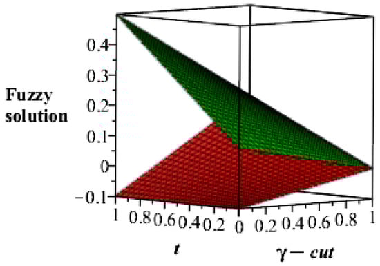
Figure 1. Lower and upper bounds fuzzy solutions of $\psi \left(t\right)$ at $\alpha =1$.

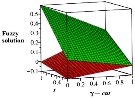
Figure 2. Lower and upper bounds fuzzy solutions of $\xi \left(t\right)$ at $\alpha =1$.

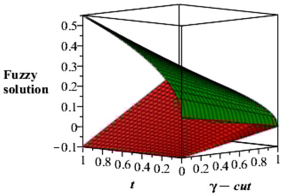
Figure 3. Lower and upper bounds fuzzy solutions of $\psi \left(t\right)$ at $\alpha =0.5$.

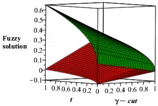
Figure 4. Lower and upper bounds fuzzy solutions of $\xi \left(t\right)$ at $\alpha =0.5$.

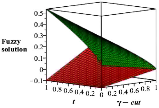
Figure 5. Lower and upper bounds fuzzy solutions of $\psi \left(t\right)$ at $\alpha =0.75$.

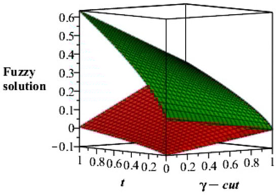
Figure 6. Lower and upper bounds fuzzy solutions of $\xi \left(t\right)$ at $\alpha =0.75$.

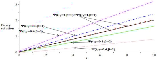
Figure 7. Lower and upper bounds interval solutions of $\psi \left(t\right)$ at $\alpha =1$.

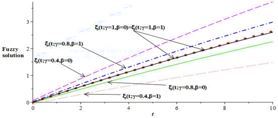
Figure 8. Lower and upper bounds interval solutions of $\xi \left(t\right)$ at $\alpha =1$.

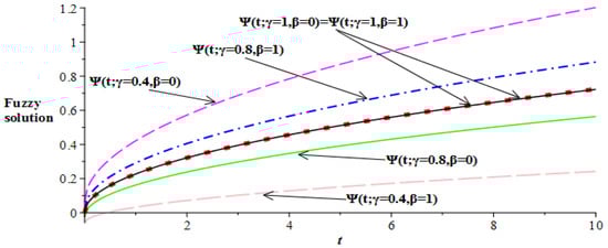
Figure 9. Lower and upper bounds interval solutions of $\psi \left(t\right)$ at $\alpha =0.5$.

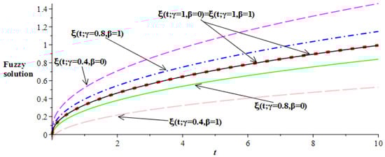
Figure 10. Lower and upper bounds interval solutions of $\xi \left(t\right)$ at $\alpha =0.5$.

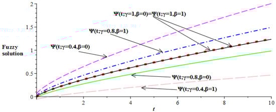
Figure 11. Lower and upper bounds interval solutions of $\psi \left(t\right)$ at $\alpha =0.75$.

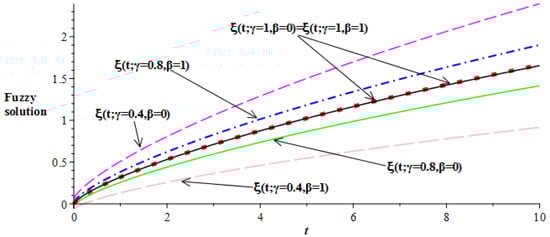
Figure 12. Lower and upper bounds interval solutions of $\xi \left(t\right)$ at $\alpha =0.75$.

Also, it can be seen that the central line (crisp result, i.e., at $\gamma -cut=1$) of Figure 7, Figure 8, Figure 9, Figure 10, Figure 11 and Figure 12 gradually decreased with a decrease in $\alpha$. Alternatively, we may say that a decrease in the values of $\alpha$ decreased the adoration of man or woman for his/her partner. From Table 1, Table 2, Table 3, Table 4, Table 5 and Table 6, it is clear that the lower and upper bounds at different values of $\alpha$ were the same at $\gamma =1$ and the obtained results matched with the solutions of Singh et al. [16] and Goyal et al. [17].

Table 1. Fuzzy and crisp solution of $\psi \left(t\right)$ at $\alpha =1$ and $\gamma =1$.

$\mathit{t}$ No of Approximation	0	0.2	0.4	0.6	0.8	1
$n=1$$\lfloor \underset{\_}{\psi },\overline{\psi }\rfloor$	[0,0]	[0.04,0.03999]	[0.08,0.07999]	[0.12,0.119999]	[0.16,0.159999]	[0.20,0.199999]
$n=2$$[\underset{\_}{\psi },\overline{\psi }\rfloor$	[0,0]	[0.04,0.04003]	[0.0801,0.0802]	[0.1203,0.120359]	[0.1606,0.16064]	[0.2009,0.20099]
$n=3$$\lfloor \underset{\_}{\psi },\overline{\psi }\rfloor$	[0,0]	[0.04,0.04003]	[0.0801,0.08015]	[0.1203,0.120342]	[0.1606,160599]	[0.2009,0.20092]
$n=4$$\lfloor \underset{\_}{\psi },\overline{\psi }\rfloor$	[0,0]	[0.04,0.04004]	[0.0801,0.08015]	[0.1203,0.120342]	[0.1606,160597]	[0.2009,0.20092]
$n=5$$\lfloor \underset{\_}{\psi },\overline{\psi }\rfloor$	[0,0]	[0.04,0.04004]	[0.0801,0.08015]	[0.1203,0.120342]	[ 0.1606,160597]	[0.2009,0.20092]
Refs. [16,17] Crisp value at $\gamma =1$	0	0.04	0.0801	0.1203	0.1606	0.2009

Table 2. Fuzzy and crisp solution of $\xi \left(t\right)$ at $\alpha =1$ and $\gamma =1$.

$\mathit{t}$ No of Approximation	0	0.2	0.4	0.6	0.8	1
$n=1$$\lfloor \underset{\_}{\xi },\overline{\xi }\rfloor$	[0,0]	[0.06,0.059999]	[0.12,0.1199]	[0.18,0.179999]	[0.24,0.239999]	[0.30,0.29999]
$n=2$$\lfloor \underset{\_}{\xi },\overline{\xi }\rfloor$	[0,0]	[0.0598,0.0598]	[0.1192,0.1197]	[0.1783,0.178389]	[0.2371,0.237189]	[0.2954,0.29549]
$n=3$$\lfloor \underset{\_}{\xi },\overline{\xi }\rfloor$	[0,0]	[0.0598,0.0598]	[0.1192,0.1192]	[0.1784,0.178406]	[0.2371,0.237182]	[0.2956,0.29562]
$n=4$$\lfloor \underset{\_}{\xi },\overline{\xi }\rfloor$	[0,0]	[0.0598,0.0598]	[0.1192,0.1192]	[0.1784,0.178405]	[0.2371,0.237179]	[0.2956,0.29561]
$n=5$$\lfloor \underset{\_}{\xi },\overline{\xi }\rfloor$	[0,0]	[0.0598,0.0598]	[0.1192,0.1192]	[0.1784,0.178405]	[0.2371,0.237179]	[0.2956,0.29561]
Refs. [16,17] Crisp value at $\gamma =1$	0	0.0598	0.1192	0.1784	0.2371	0.2956

Table 3. Fuzzy and crisp solution of $\psi \left(t\right)$ at $\alpha =0.5$.

$\mathit{t}$ $\mathit{\gamma }-\mathbf{cut}$	0	0.2	0.4	0.6	0.8	1
$\gamma =0$$\lfloor \underset{\_}{\psi },\overline{\psi }\rfloor$	[−0.1,0.1]	[−0.991,0.3016]	[−0.0985,0.3853]	[−0.0980,0.4496]	[−0.0975,0.5038]	[−0.0970,0.5515]
$\gamma =0.2$$\lfloor \underset{\_}{\psi },\overline{\psi }\rfloor$	[−0.08,0.08]	[−0.059,0.2616]	[−0.0501,0.3370]	[−0.0432,0.3949]	[−0.0373,0.4437]	[−0.0321,0.4867]
$\gamma =0.4$$\lfloor \underset{\_}{\psi },\overline{\psi }\rfloor$	[−0.06,0.06]	[−0.0189,0.2215]	[−0.0017,0.2886]	[0.0115,0.3401]	[0.0228,0.3836]	[0.0328,0.4219]
$\gamma =0.6$$\lfloor \underset{\_}{\psi },\overline{\psi }\rfloor$	[−0.04,0.04]	[0.0211,0.1814]	[0.0467,0.2402]	[0.0663,0.2854]	[0.0829, 0.3234]	[0.0976,0.3570]
$\gamma =0.8$$\lfloor \underset{\_}{\psi },\overline{\psi }\rfloor$	[−0.02,0.02]	[0.0613,0.1414]	[0.0950,0.1918]	[0.1211,0.2306]	[0.1431,0.2633]	[0.1625, 0.2922]
$\gamma =1$$\lfloor \underset{\_}{\psi },\overline{\psi }\rfloor$	[0,0]	[0.1013,0.1013]	[0.1434, 0.1434]	[0.1759, 0.1758]	[0.2032, 0.2032]	[0.2273, 0.2273]
Refs. [16,17] Crisp value at $\gamma =1$	0	0.1013	0.1434	0.1759	0.2032	0.2273

Table 4. Fuzzy and crisp solution of $\xi \left(t\right)$ at $\alpha =0.5$.

$\mathit{t}$ $\mathit{\gamma }-\mathbf{cut}$	0	0.2	0.4	0.6	0.8	1
$\gamma =0$$\lfloor \underset{\_}{\xi },\overline{\xi }\rfloor$	[−0.1,0.1]	[−0.0500,0.3493]	[−0.0299,0.4511]	[−0.0146,0.5288]	[−0.0019,0.5938]	[0.0092,0.6509]
$\gamma =0.2$$\lfloor \underset{\_}{\xi },\overline{\xi }\rfloor$	[−0.08,0.08]	[−0.0101,0.3094]	[0.0182,0.4030]	[0.0397,0.4744]	[0.0577, 0.5343]	[0.0734,0.5867]
$\gamma =0.4$$\lfloor \underset{\_}{\xi },\overline{\xi }\rfloor$	[−0.06,0.06]	[0.0298,0.2694]	[0.0663,0.3549]	[0.0940,0.4200]	[0.1172,0.4747]	[0.1375,0.5226]
$\gamma =0.6$$\lfloor \underset{\_}{\xi },\overline{\xi }\rfloor$	[−0.04,0.04]	[0.0698,0.2295]	[0.1144,0.3068]	[0.1484,0.3657]	[0.1768,0.4151]	[0.2017, 0.4584]
$\gamma =0.8$$\lfloor \underset{\_}{\xi },\overline{\xi }\rfloor$	[−0.02,0.02]	[0.1097,0.1896]	[0.1625,0.2587]	[0.2027,0.3114]	[0.2364,0.355]	[0.2659, 0.3942]
$\gamma =1$$\lfloor \underset{\_}{\xi },\overline{\xi }\rfloor$	[0,0]	[0.1496,0.1496]	[0.2106,0.2106]	[0.2570,0.2570]	[0.2960,0.2960]	[0.3300,0.3300]
Refs. [16,17] Crisp value at $\gamma =1$	0	0.1496	0.2106	0.2570	0.2960	0.3300

Table 5. Fuzzy and crisp solution of $\psi \left(t\right)$ at $\alpha =0.75$.

$\mathit{t}$ $\mathit{\gamma }-\mathbf{cut}$	0	0.2	0.4	0.6	0.8	1
$\gamma =0$$\lfloor \underset{\_}{\psi },\overline{\psi }\rfloor$	[−0.1,0.1]	[−0.0995,0.2210]	[−0.0991,0.3187]	[−0.0986,0.3965]	[−0.0980,0.4681]	[−0.0974,0.5353]
$\gamma =0.2$$\lfloor \underset{\_}{\psi },\overline{\psi }\rfloor$	[−0.08,0.08]	[−0.0666,0.1970]	[−0.0573,0.2769]	[−0.0491,0.3470]	[−0.0414,0.4115]	[−0.0342,0.4720]
$\gamma =0.4$$\lfloor \underset{\_}{\psi },\overline{\psi }\rfloor$	[−0.06,0.06]	[−0.0336,0.1640]	[−0.0155,0.2351]	[0.0005,0.2975]	[0.0152,0.3549]	[0.0291,0.4087]
$\gamma =0.6$$\lfloor \underset{\_}{\psi },\overline{\psi }\rfloor$	[−0.04,0.04]	[−0.0007,0.1311]	[0.0263,0.1933]	[0.0410,0.2480]	[0.0718,0.2983]	[0.0924,0.3455]
$\gamma =0.8$$\lfloor \underset{\_}{\psi },\overline{\psi }\rfloor$	[−0.02,0.02]	[0.0323,0.0982]	[0.0680,0.1516]	[0.0995,0.1985]	[0.12843,0.2417]	[0.1557,0.2822]
$\gamma =1$$\lfloor \underset{\_}{\psi },\overline{\psi }\rfloor$	[0,0]	[0.0652,0.0652]	[0.1098,0.1098]	[0.1490,0.1490]	[0.1850,0.1850]	[0.2189,0.2189]
Refs. [16,17] Crisp value at $\gamma =1$	0	0.0652	0.1098	0.1490	0.1850	0.2189

Table 6. Fuzzy and crisp solution of $\xi \left(t\right)$ at $\alpha =0.75$.

$\mathit{t}$ $\mathit{\gamma }-\mathbf{cut}$	0	0.2	0.4	0.6	0.8	1
$\gamma =0$$\lfloor \underset{\_}{\xi },\overline{\xi }\rfloor$	[−0.1,0.1]	[−0.0675,0.2615]	[−0.0457,0.3707]	[−0.0268,0.4658]	[−0.0097,0.5526]	[0.0063,0.6336]
$\gamma =0.2$$\lfloor \underset{\_}{\xi },\overline{\xi }\rfloor$	[−0.08,0.08]	[−0.0346,0.2286]	[−0.0040,0.3290]	[0.0225,0.4165]	[0.0466,0.4963]	[0.0690,0.5709]
$\gamma =0.4$$\lfloor \underset{\_}{\xi },\overline{\xi }\rfloor$	[−0.06,0.06]	[−0.0017,0.1957]	[0.0376,0.2874]	[0.0717,0.3672]	[0.1028,0.4401]	[0.1317,0.5081]
$\gamma =0.6$$\lfloor \underset{\_}{\xi },\overline{\xi }\rfloor$	[−0.04,0.04]	[0.0312,0.1628]	[0.0792,0.2457]	[0.1210,0.3179]	[0.1590,0.3839]	[0.1945,0.4454]
$\gamma =0.8$$\lfloor \underset{\_}{\xi },\overline{\xi }\rfloor$	[−0.02,0.02]	[0.0641,0.1299]	[0.1209,0.2041]	[0.1702,0.2687]	[0.2152,0.3276]	[0.2572,0.3827]
$\gamma =1$$\lfloor \underset{\_}{\xi },\overline{\xi }\rfloor$	[0,0]	[0.0970,0.0970]	[0.1625,0.1625]	[0.2195, 0.2195]	[0.2714,0.2714]	[0.3199,0.3199]
Refs. [16,17] Crisp value at $\gamma =1$	0	0.097	0.1625	0.2195	0.2714	0.3199

6. Conclusions

In this paper, approximate solutions of a fuzzy FDMM were found with the help of an efficient method, namely FRDTM. In the procedure, the DPF of fuzzy number was applied. This methodology was found to be straight forward as it converted FDEs to an advantageous form involving two parameters that controlled the uncertainty. Attained outcomes were compared with the existing results and were found to be in agreement. The main benefit of applying this method is that it does not require any assumption, perturbation, or discretization for solving the governing time-fractional dynamical model. Also, the computation time was less compared to other techniques. From this study, it is concluded that the decrease in the values of $\alpha$ decreased romantic relations between the couple.

References

- Jena, R.M.; Chakraverty, S.; Jena, S.K. Dynamic Response Analysis of Fractionally Damped Beams Subjected to External Loads using Homotopy Analysis Method. J. Appl. Comput. Mech. 2019, 5, 355–366. [Google Scholar]
- Jena, R.M.; Chakraverty, S. Solving time-fractional Navier–Stokes equations using homotopy perturbation Elzaki transform. SN Appl. Sci. 2019, 1, 16. [Google Scholar] [CrossRef]
- Jena, R.M.; Chakraverty, S. Residual Power Series Method for Solving Time-fractional Model of Vibration Equation of Large Membranes. J. Appl. Comput. Mech. 2019, 5, 603–615. [Google Scholar]
- Jena, R.M.; Chakraverty, S. A new iterative method based solution for fractional Black–Scholes option pricing equations (BSOPE). SN Appl. Sci. 2019, 1, 95–105. [Google Scholar] [CrossRef]
- Edeki, S.O.; Motsepa, T.; Khalique, C.M.; Akinlabi, G.O. The Greek parameters of a continuous arithmetic Asian option pricing model via Laplace Adomian decomposition method. Open Phys. 2018, 16, 780–785. [Google Scholar] [CrossRef]
- Podlubny, I. Fractional Differential Equations; Academic Press: San Diego, CA, USA, 1999. [Google Scholar]
- Kilbas, A.A.; Srivastava, H.M.; Trujillo, J.J. Theory and Applications of Fractional Differential Equations; North-Holland Mathematical Studies; Elsevier Science Publishers: Amsterdam, The Netherlands; London, UK; New York, NY, USA, 2006; Volume 204. [Google Scholar]
- Baleanu, D.; Diethelm, K.; Scalas, E.; Trujillo, J.J. Fractional Calculus: Models and Numerical Methods; World Scientific: Boston, MA, USA: 2012. [Google Scholar]
- Baleanu, D.; Machado, J.A.T.; Luo, A.C. Fractional Dynamics and Control; Springer: Berlin, Germany, 2012. [Google Scholar]
- Miller, K.S.; Ross, B. An Introduction to the Fractional Calculus and Fractional Differential Equations; A Wiley-Interscience Publication; John Wiley and Sons: New York, NY, USA; Chichester, UK; Brisbane, Australian; Toronto, ON, Canada; Singapore, 1993. [Google Scholar]
- Barley, K.; Cherif, A. Stochastic nonlinear dynamics of interpersonal and romantic relationships. Appl. Math. Comput. 2011, 217, 6273–6281. [Google Scholar] [CrossRef]
- Rinaldi, S. Love dynamics: The case of linear couples. Appl. Math. Comput. 1998, 95, 181–192. [Google Scholar] [CrossRef]
- Ozalp, N.; Koca, I. A fractional order nonlinear dynamical model of interpersonal relationships. Adv. Differ. Equ. 2012, 189, 1–7. [Google Scholar] [CrossRef]
- Khader, M.M.; Alqahtani, R. Approximate solution for system of fractional non-linear dynamical marriage model using Bernstein polynomials. J. Nonlinear Sci. Appl. 2017, 10, 865–873. [Google Scholar] [CrossRef][Green Version]
- Khader, M.M.; Shloof, A.; Ali, H. On the numerical simulation and convergence study for system of non-linear fractional dynamical model of marriage. NTMSCI 2017, 5, 130–141. [Google Scholar] [CrossRef]
- Singh, J.; Kumar, D.; Qurashi, M.A.; Baleanu, D. A Novel Numerical Approach for a Nonlinear Fractional Dynamical Model of Interpersonal and Romantic Relationships. Entropy 2017, 19, 375. [Google Scholar] [CrossRef]
- Goyal, M.; Prakash, A.; Gupta, S. Numerical simulation for time-fractional nonlinear coupled dynamical model of romantic and interpersonal relationships. Pramana J. Phys. 2019, 92, 82. [Google Scholar] [CrossRef]
- Martin, M.T.C.; Bumpass, B.L. Recent trends in marital disruption. Demography 1989, 26, 37–51. [Google Scholar] [CrossRef] [PubMed]
- Strogatz, S.H. Nonlinear Dynamics and Chaos: With Applications to Physics, Biology, Chemistry and Engineering; Reading, M.A., Ed.; Addison-Wesley: Boston, MA, USA, 1994. [Google Scholar]
- Gottman, J.M.; Murray, J.D.; Swanson, C.C.; Tyson, R.; Swanson, K.R. The Mathematics of Marriage; MIT Press: Cambridge, MA, USA, 2002. [Google Scholar]
- Chang, S.L.; Zadeh, L.A. On fuzzy mapping and control. IEEE Trans. Syst. Man Cybern. 1972, 2, 30–34. [Google Scholar] [CrossRef]
- Dubois, D.; Prade, H. Towards fuzzy differential calculus part 3: Differentiation. Fuzzy Sets Syst. 1982, 8, 225–233. [Google Scholar] [CrossRef]
- Kaleva, O. The Cauchy problem for fuzzy differential equations. Fuzzy Sets Syst. 1990, 35, 389–396. [Google Scholar] [CrossRef]
- Seikkala, S. On the fuzzy initial value problem. Fuzzy Sets Syst. 1987, 24, 319–330. [Google Scholar] [CrossRef]
- Chakraverty, S.; Tapaswini, S.; Behera, D. Fuzzy Arbitrary Order System: Fuzzy Fractional Differential Equations and Applications; John Wiley & Sons Inc.: Hoboken, NJ, USA, 2016. [Google Scholar]
- Chakraverty, S.; Tapaswini, S.; Behera, D. Fuzzy Differential Equations and Applications for Engineers and Scientists; Taylor and Francis Group: Boca Raton, FL, USA, 2016. [Google Scholar]
- Chakraverty, S.; Sahoo, D.M.; Mahato, N.R. Concepts of Soft Computing: Fuzzy and ANN with Programming; Springer: Singapore, 2019. [Google Scholar]
- Momani, S.; Odibat, Z. A generalized differential transform method for linear partial differential equations of fractional order. Appl. Math. Lett. 2008, 21, 194–199. [Google Scholar]
- Singh, B.K.; Kumar, P. FRDTM for numerical simulation of multi-dimensional, time-fractional model of Navier–Stokes equation. Ain Shams Eng. J. 2018, 9, 827–834. [Google Scholar] [CrossRef]
- Singh, J.; Kumar, D.; Swroop, R.; Kumar, S. An efficient computational approach for time-fractional Rosenau–Hyman equation. Neural Comput. Appl. 2018, 30, 3063–3070. [Google Scholar] [CrossRef]
- Rawashdeh, M.S. An Efficient Approach for Time–Fractional Damped Burger and Time—Sharma—Tasso—Olver Equations Using the FRDTM. Appl. Math. Inf. Sci. 2015, 9, 1239–1246. [Google Scholar]
- Keskin, Y.; Oturan, G. Reduced Differential Transform Method for Partial Differential Equations. Int. J. Nonlinear Sci. Numer. Simul. 2009, 10, 741–749. [Google Scholar] [CrossRef]
© 2019 by the authors. Licensee MDPI, Basel, Switzerland. This article is an open access article distributed under the terms and conditions of the Creative Commons Attribution (CC BY) license (http://creativecommons.org/licenses/by/4.0/).