Non-Stationary Fractal Interpolation

Center of Mathematics, Technical University of Munich, 85748 Garching, Germany
Mathematics 2019, 7(8), 666; https://doi.org/10.3390/math7080666
Submission received: 1 July 2019
/
Revised: 17 July 2019
/
Accepted: 24 July 2019
/
Published: 25 July 2019
(This article belongs to the Special Issue Fractals: Geometry, Analysis and Mathematical Physics)
Abstract
:We introduce the novel concept of a non-stationary iterated function system by considering a countable sequence of distinct set-valued maps where each maps and arises from an iterated function system. Employing the recently-developed theory of non-stationary versions of fixed points and the concept of forward and backward trajectories, we present new classes of fractal functions exhibiting different local and global behavior and extend fractal interpolation to this new, more flexible setting.
1. Introduction
Contractive operators on complete function spaces play a crucial role in the theory of differential and integral equations and are essential for the development of iterative solvers. One class of such contractive operators is defined on the graphs of functions using a particular type of iterated function system (IFS). The fixed points of such IFSs are graphs of functions that exhibit fractal characteristics. There exists an extensive literature on IFSs and fractal functions including, for instance, [1,2,3].
Up to now, the construction of contractive operators on sets or functions uses primarily sequences of iterates of one operator. Recently, motivated by non-stationary subdivision algorithms, a more general class of sequences consisting of different contractive operators was introduced in [4] and their limit properties studied. These ideas were then extended in [5] to sequences of different contractive operators mapping between different spaces. Using different contractive operators provide one with the ability to construct limit attractors that have different shapes or features at different scales.
This article uses the aforementioned new ideas to introduce the novel concept of non-stationary IFS and non-stationary fractal interpolation. These new ideas widen the applicability of fractal functions and fractal interpolation as they now include scale- and location-dependent features.
The outline of this paper is as follows. After providing some necessary preliminaries in Section 2, some results from [4] are presented in Section 3. In Section 4, (stationary) fractal interpolation and the associated (stationary) IFSs are reviewed. Non-stationary fractal functions are constructed in Section 5, and non-stationary fractal interpolation is introduced in Section 6. The final Section 7 defines non-stationary fractal functions on the Bochner–Lebesgue -spaces with .
2. Preliminaries
Let be a complete metric space. Given a map , the Lipschitz constant associated with f is defined by:
The map f is called Lipschitz if and a contraction on X if .
Definition 1.
Let be a complete metric space and a finite family of contractions on X. Then, the pair is called a contractive iterated function system (IFS) on X.
Remark 1.
As we deal exclusively with contractive IFSs in this article, we drop the adjective “contractive” in the following.
Remark 2.
In order to avoid trivialities, we henceforth assume that the number of maps in an IFS is an integer greater than one.
With an IFS and its point maps , we can associate a set-valued mapping, also denoted by , as follows. Let be the hyperspace of all nonempty compact subsets of X endowed with the Hausdorff–Pompeiu metric:
where .
It is known that for contractive mappings , the set-valued map defined by (1) is a contractive Lipschitz map on with Lipschitz constant . Here, we set . Moreover, the completeness of implies the completeness of .
The next definition is motivated by the validity of the Banach fixed point theorem in the above setting.
Definition 2.
The unique fixed point of the contractive set-valued map is called the attractor of the IFS .
Note that since A satisfies the self-referential equation:
the attractor is in general a fractal set.
It follows directly from the proof of the Banach fixed point theorem that the attractor A is obtained as the limit (in the Hausdorff–Pompeiu metric) of the iterative process , :
for an arbitrary . Here, denotes the k-fold composition of with itself.
3. Systems of Function Systems
In [4], a generalization of IFSs was presented. The idea for this generalization comes from the theory of subdivision schemes. Instead of using only one set-valued map to obtain an iterative process with initial , a sequence of function systems consisting of different families is considered.
To this end, let be a complete metric space and a sequence of transformations .
Definition 3.
([4], Definition 3.6) Let be a sequence of transformations . A subset of X is called an invariant set of the sequence if:
A criterion for obtaining an invariant domain for a sequence of transformations on X is given below.
Proposition 1.
([4], Lemma 3.7) Let be a sequence of transformations on . Suppose there exists a such that for all :
for some and . Then, the ball of radius centered at q is an invariant set for .
Proof.
For the proof, we refer the interested reader to [4]. □
Now, suppose that is a sequence of set-valued maps defined by:
where is a family of contractions constituting an IFS on a complete metric space . Setting , we obtain that .
The following definitions are taken from [4] (Section 4).
Definition 4.
Let . The sequences:
and:
are called the forward and backward trajectories of , respectively.
For our current setting, it was shown in ([4], Corollary 4.2) that if:
- (i)
- , for all ;
- (ii)
- there exists a common nonempty compact invariant set for the maps , , , such that converges uniformly on to as ;
- (iii)
- the IFS with is contractive on ;
then the forward trajectory converges for an arbitrary to the unique attractor of .
It was observed in [4] that the limits of forward trajectories do not lead to new classes of fractals. On the other hand, backward trajectories converge under rather mild conditions, even when forward trajectories do not converge to a (contractive) IFS, and generate new types of fractal sets.
As the convergence of backward trajectories is important for this article, we summarize the result in the next theorem, whose proof the reader can find in [4].
Theorem 1.
([4], Corollary 4.4) Let be a family of set-valued maps of the form (4) whose elements are collections of contractions constituting IFSs on a complete metric space . Suppose that:
- (i)
- there exists a nonempty closed invariant set for , , ;
- (ii)
- and:
Then, the backward trajectories converge for any initial to a unique attractor .
Remark 3.
Remark 4.
The conditions for convergence of the forward and backward trajectories are more general in [4]. For our purposes and setting, the above criteria are however sufficient.
Remark 5.
Fractals generated by backwards trajectories allow for more flexibility in their shapes. By a proper choice of IFSs, one can construct fractals exhibiting different local behavior (cf. [4]). This is due to the fact that in the sequence:
the global shape of the attractor is determined by the initial maps , whereas the local shape is given by the final maps . Thus, scaling the attractor by , , reveals the behavior of the attractor of . See also [4] (Example 5.1).
Remark 6.
A comparison to V-variable fractals [7] was also undertaken in [4] (Section 4.1), showing that systems of function systems (SFSs) have weaker prerequisites than V-variable fractals.
4. Fractal Interpolation
Before introducing the new concept of non-stationary fractal interpolation, we need to briefly recall the rudimentaries of (stationary) fractal interpolation and (stationary) fractal functions. This is the purpose of the current section.
4.1. Stationary Fractal Interpolation
Suppose we are given a finite family of injective contractions generating a partition of X in the sense that:
Let be a complete metric space with metric . A map is called bounded (with respect to the metric ) if there exists a constant such that for all , .
Recall that the set becomes a complete metric space when endowed with the metric:
Remark 7.
Under the usual addition and scalar multiplication of functions, the space is actually a metric linear space, i.e., a vector space for which the operations of vector addition and scalar multiplication are continuous (see, for instance, [8]).
For , let be a mapping that is uniformly contractive in the second variable, i.e., there exists a so that for all :
Define an operator by:
where denotes the characteristic function of a set M. Such operators are referred to as Read–Bajractarević (RB) operators. The operator T is well defined, and since g is bounded and each contractive in the second variable, .
Equivalently, (12) can also be expressed in the form:
To achieve notational simplicity, we set in the above equation.
Therefore, by the Banach fixed point theorem, T has a unique fixed point in . This unique fixed point is called the bounded fractal function (generated by T), and it satisfies the self-referential equation:
or, equivalently,
The fixed point is obtained as the limit of the sequence of mappings:
where is arbitrary.
Next, we would like to consider a special choice for the mappings . To this end, we require the concept of an F-space. We recall that a metric is called complete if every Cauchy sequence in Y converges (with respect to d) to a point of Y, and translation-invariant if:
Now, assume that Y is an F-space, i.e., a topological vector space whose topology is induced by a complete translation-invariant metric d and, in addition, that this metric is homogeneous. This setting allows us to consider mappings of the form:
where and is a function.
The metric is homogeneous, and therefore, the mappings (18) satisfy condition (11) if the functions are assumed to be bounded on X with bounds in . For then:
Here, denotes the supremum norm and . Henceforth, we will assume that all functions are bounded above by .
Next, we exhibit the relationship between the graph of the fixed point of the operator T given by (12) and the attractor of an associated contractive IFS.
To this end, consider the complete metric space , and define mappings by:
Assume that the mappings in addition to being uniformly contractive in the second variable are also uniformly Lipschitz continuous in the first variable, i.e., there exists a constant such that for all ,
Denote by the largest of the contractivity constants of the , and let . Then, the mapping given by:
is a metric on compatible with the product topology on .
The next theorem is a special case of a result presented in [9].
Theorem 2.
Conversely, assume that is an IFS whose maps are of the form (21) where the functions are contractive injections satisfying (8) and (9), and the mappings are uniformly Lipschitz continuous in the first variable and uniformly contractive in the second variable. Thus, an RB operator of the form (12) can be associated with the IFS . The attractor of is then the graph of the fixed point f of (this was the original approach in [10] to define a fractal interpolation function on a compact interval in ). The diagram (23) is then commutative with replaced by and T replaced by .
We now specialize even further and choose arbitrary and set:
Then, the RB operator T becomes:
and under the assumption that , its unique fixed point satisfies the self-referential equation:
Remark 8.
The functions f and b are referred to as the seed and base function, respectively.
Remark 9.
The fixed point in (26) clearly depends on the seed function f, the base function b, and the scaling functions . Fixing f and b, but varying generate an uncountable family of fractal functions originating from .
In the case of univariate fractal interpolation on the real line with , , the base function b can be chosen to be the affine function whose graph connects the points and .
If we consider the complete metric space of continuous functions instead of , define:
and impose the join-up conditions:
the fixed point will be a continuous function whose graph interpolates the set . Such functions are usually referred to as fractal interpolation functions [6,10]. As the RB operator is the same at each level of recursion (17), we refer to this as stationary fractal interpolation.
5. Non-Stationary Fractal Functions
Here, we introduce non-stationary versions of the concepts of fractal functions as presented in the previous section.
To this end, consider a doubly-indexed family of injective contractions from generating a partition of X for each in the sense of (8) and (9).
Suppose that Y is an F-space, and is such that:
For each , define an RB operator by:
It is straightforward to verify that each RB operator is a contraction on with Lipschitz constant:
Proposition 2.
Let be a sequence of RB operators of the form (28) on . Suppose that the elements of satisfy:
for some . Then, the ball of radius centered at is an invariant set for .
Proof.
Note that since Y is an F-space, we have for all ,
Now, let . Then, there exists an with . Thus, for any ,
By (31), is uniformly bounded in by . As the metric is homogeneous,
which shows, after taking the sup over , that . Proposition 1 now yields the statement. □
Considering the backward trajectories of the sequence of RB operators defined above and using Theorem 1, we obtain the next result.
Theorem 3.
The backwards trajectories converge for any initial to a unique attractor , where is the closed ball in of radius centered at zero.
Proof.
By Theorem 1, it remains to show that converges. This, however, follows directly from (30):
□
A fixed point generated by a sequence of different RB operators will be called a non-stationary fractal function (of class ).
Remark 10.
Item (b) in Remark 3, of course, also applies to a sequence of RB operators , thus allowing the construction of more general fractal functions exhibiting different local behavior at different scales.
Example 1.
Let and . Consider the two RB operators:
and:
For both operators, , .
It is known that , where τ denotes the Takagi function [11], and that , where .
Consider the alternating sequence of RB operators given by:
Two images of this hybrid attractor of the backward trajectory starting with are shown in Figure 1.
6. Non-Stationary Fractal Interpolation
Let us now consider the case and . Both spaces are metrizable under the usual Euclidean distance. In the following, we consider a sequence of RB operators of the form (25) acting on an appropriate metric subspace of . Our emphasis here lies in the construction of attractors that are continuous functions on . For this purpose, we need to impose conditions on the RB operators that guarantee global continuity of the iterates across .
For , let be a family of injections from generating a partition of in the sense of (8) and (9). Assume w.l.o.g. that and , and define:
where and . By relabeling, if necessary, we may assume that .
Let be arbitrary. Define a metric subspace of by:
and note that becomes a complete linear metric space when endowed with the metric induced by the sup-norm on continuous functions. Additionally, let be the unique affine function whose graph connects the points and :
Further, let , where , be a family of sets of points in . For , define an RB operator by:
where such that
Note that we have the continuity of at the points :
For,
and
Therefore, , and interpolates in the sense that:
Remark 11.
Denote by the IFS given by the maps , and observe that, for each , the attractor of is the interval . The invariant set, in , for is given by . Hence, all backward trajectories converge to as (as do all forward trajectories).
Proposition 3.
Proof.
In connection with Theorem 3, the above arguments prove the next result.
Theorem 4.
We refer to the fixed point as a continuous non-stationary fractal interpolation function.
To illustrate the above results, we refer to Remark 3(c) and present the following example.
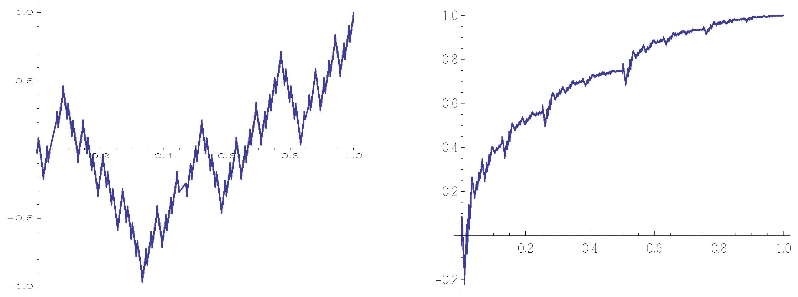
Example 2.
Here, we consider the two RB operators , , given by:
and
The RB operators and generate Kiesswetter’s fractal function [12] and a Casino function [13], respectively.
Consider again the alternating sequence of RB operators given by:
Two images of the hybrid attractor of the backward trajectory starting with the function , , are shown below in Figure 2.
Remark 12.
Theorem 2 holds in the case of non-stationary fractal functions as well. For , a non-stationary IFS is associated with by setting:
The conditions imposed on and the form of the second component allow the immediate transfer of the proof of Theorem 2. Hence, even in the non-stationary case, one may choose the geometry (IFS) or the analytic (RB operator) approach when defining non-stationary fractal functions.
7. Non-Stationary Fractal Functions in Bochner–Lebesgue Spaces
In this section, we construct non-stationary fractal functions in the Bochner–Lebesgue spaces with . To this end, suppose that X is a closed subspace of a Banach space and a measure space. Further, suppose that is a Banach space.
Recall that the Bochner–Lebesgue space , is comprised of all Bochner measurable functions such that:
and
For , the spaces are defined using a metric instead of a norm to obtain completeness. More precisely, for , define by:
Then, becomes an F-space (note that the inequality holds for all ). For more details, we refer to [14,15].
In order to work in both cases simultaneously, we define by:
with the usual modification for .
We use the notation and terminology of Section 5 and assume that:
- (A1)
- ;
- (A2)
- ;
- (A3)
If we define for each an RB operator on of the form (28), whose maps satisfy assumptions (A1), (A2), and (A3), then a straightforward computation shows that has the following Lipschitz constants on :
where denotes the Lipschitz constant of and D the Fréchet derivative on X.
Now, set:
Imposing the condition:
for some and further requiring that:
yield by Proposition 2 an invariant set for , namely the closed -ball:
The above elaborations now prove the following theorem.
Theorem 5.
Proof.
Only (7) needs to be established. This, however, carries over directly from the proof of Theorem 3 with instead of s. □
The attractor whose existence is guaranteed by Theorem 5 is called a non-stationary fractal function of class .
Funding
This research received no external funding.
Acknowledgments
The author would like to thank Nira Dyn and David Levin for two visits to the Mathematics Department of Tel Aviv University, where the mathematical ideas for this article originated.
Conflicts of Interest
The author declares no conflict of interest.
References
- Barnsley, M.F. Fractals Everywhere; Academic Press: Orlando, FL, USA, 1988. [Google Scholar]
- Massopust, P.R. Interpolation and Approximation with Splines and Fractals; Oxford University Press: Oxford, MA, USA, 2010. [Google Scholar]
- Massopust, P.R. Fractal Functions, Fractal Surfaces, and Wavelets, 2nd ed.; Academic Press: San Diego, CA, USA, 2016. [Google Scholar]
- Levin, D.; Dyn, N.; Viswanathan, P. Non-stationary versions of fixed-point theory, with applications to fractals and subdivision. J. Fixed Point Theory Appl. 2019, 21, 1–25. [Google Scholar] [CrossRef]
- Dira, N.; Levin, D.; Massopust, P. Attractors of Trees of Maps and of Sequences of Maps between Spaces and Applications to Subdivision. Available online: http://arxiv.org/abs/1902.03407 (accessed on 9 February 2019).
- Hutchinson, J.E. Fractals and self-similarity. Indiana Univ. Math. J. 1981, 30, 713–747. [Google Scholar] [CrossRef]
- Barnsley, M.F.; Hutchinson, J.E.; Stenflo, Ö. V-variable fractals: Fractals with partial self-similarity. Adv. Math. 2008, 218, 2015–2088. [Google Scholar] [CrossRef]
- Rolewicz, S. Metric Linear Spaces; Kluwer Academic: Warsaw, Poland, 1985. [Google Scholar]
- Barnsley, M.F.; Hegland, M.; Massopust, P.R. Numerics and Fractals. Bull. Inst. Math. Acad. Sin. (N.S.) 2014, 9, 389–430. [Google Scholar]
- Barnsley, M.F. Fractal functions and interpolation. Constr. Approx. 1986, 2, 303–329. [Google Scholar] [CrossRef]
- Takagi, T. A simple example of the continuous function without derivative. Proc. Phys. Math. Soc. Jpn. 1903, 1, 176–177. [Google Scholar]
- Kiesswetter, K. Ein einfaches Beispiel für eine Funktion welche überall stetig und nicht differenzierbar ist. Math. Phys. Semesterber. 1966, 13, 216–221. [Google Scholar]
- Dubins, L.E.; Savage, L.J. Inequalities for Stochastic Processes; Dover Publications: New York, NY, USA, 1976. [Google Scholar]
- Rudin, W. Functional Analysis; McGraw–Hill: New York, NY, USA, 1991. [Google Scholar]
- Adams, R.; Fourier, J. Sobolev Spaces, 2nd ed.; Academic Press: New York, NY, USA, 2003. [Google Scholar]
Figure 1.
The hybrid attractor. It is smooth at one scale (Left), but fractal at another (Right).
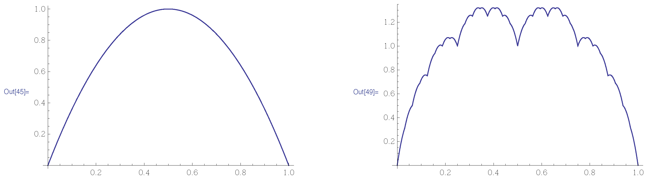
Figure 2.
The hybrid Kiesswetter–Casino attractor. The graph of the Casino function (Right) contains at the fine scale images of the Kiesswetter function (Left).
Figure 2.
The hybrid Kiesswetter–Casino attractor. The graph of the Casino function (Right) contains at the fine scale images of the Kiesswetter function (Left).
© 2019 by the author. Licensee MDPI, Basel, Switzerland. This article is an open access article distributed under the terms and conditions of the Creative Commons Attribution (CC BY) license (http://creativecommons.org/licenses/by/4.0/).
Share and Cite
MDPI and ACS Style
Massopust, P. Non-Stationary Fractal Interpolation. Mathematics 2019, 7, 666. https://doi.org/10.3390/math7080666
AMA Style
Massopust P. Non-Stationary Fractal Interpolation. Mathematics. 2019; 7(8):666. https://doi.org/10.3390/math7080666
Chicago/Turabian StyleMassopust, Peter. 2019. "Non-Stationary Fractal Interpolation" Mathematics 7, no. 8: 666. https://doi.org/10.3390/math7080666
APA StyleMassopust, P. (2019). Non-Stationary Fractal Interpolation. Mathematics, 7(8), 666. https://doi.org/10.3390/math7080666
Note that from the first issue of 2016, this journal uses article numbers instead of page numbers. See further details here.