On the Gibbs Effect Based on the Quasi-Affine Dual Tight Framelets System Generated Using the Mixed Oblique Extension Principle

Abstract

Gibbs effect represents the non-uniform convergence of the nth Fourier partial sums in approximating functions in the neighborhood of their non-removable discontinuities (jump discontinuities). The overshoots and undershoots cannot be removed by adding more terms in the series. This effect has been studied in the literature for wavelet and framelet expansions. Dual tight framelets have been proven useful in signal processing and many other applications where translation invariance, or the resulting redundancy, is very important. In this paper, we will study this effect using the dual tight framelets system. This system is generated by the mixed oblique extension principle. We investigate the existence of the Gibbs effect in the truncated expansion of a given function by using some dual tight framelets representation. We also give some examples to illustrate the results.

1. Introduction

The Gibbs effect was first recognized over a century ago by Henry Wilbraham in 1848 (see Ref. [1]). However, in 1898 Albert Michelson and Samuel Stratton (see Ref. [2]) observed it via a mechanical machine that they used to calculate the Fourier partial sums of a square wave function. Soon after, Gibbs explained this effect in two publications [3,4]. In his first short paper, Gibbs failed to notice the phenomenon and the limits of the graphs of the Fourier partial sums was inaccurate. In the second paper, he published a correction and gave the description of overshoot at the point of jump discontinuity. In fact, Gibbs did not provide a proof for his argument but only in 1906 a detailed mathematical description of the effect was introduced and named after Gibbs phenomenon by Maxime (see Ref. [5]) as he believed Gibbs to be the first person noticing it. This phenomenon has been studied extensively in Fourier series and many other situations such as the classical orthogonal expansions (see Refs. [6,7,8]), spline expansion (see Refs. [9,10]), wavelets and framelets series (see Refs. [11,12,13,14,15,16,17]), sampling approximations (see Ref. [18]), and many other theoretical investigations (see Refs. [19,20,21,22,23]). By considering Fourier series, it is impossible to recover accurate point values of a periodic function with many finitely jump discontinuities from its Fourier coefficients. Wavelets and their generalizations (framelets) have great success in coefficients recovering and have many applications in signal processing and numerical approximations (see Refs. [24,25,26,27]). However, many of these applications are represented by smooth functions that have jump discontinuities. However, expanding these functions will create (most often) unpleasant ringing effect near the gaps. It is the aim of this article to analyze the Gibbs effect of dual tight framelets using a different/higher order of vanishing moments.

Let us recall the preliminary background by introducing some notations (e.g., see Refs. [28,29,30]). Let $L_2\left(\mathbb{R}\right)$ denote the space of all square integrable functions over the space $\mathbb{R}$, where

$$L_2\left(\mathbb{R}\right)=\left\{f:\mathbb{R}\to \mathbb{R};{\int }_{\mathbb{R}}{\left|f\right|}^2<\infty \right\}.$$

Definition 1

([31]). Let $\psi \in L_2\left(\mathbb{R}\right)$. For $j,k\in \mathbb{Z}$, define the function ${\psi }_{j,k}$ by

$${\psi }_{j,k}=2^{j/2}\psi (2^j·-k).$$

Then, we say the function ψ is a wavelet if the set ${\left\{{\psi }_{j,k}\right\}}_{j,k\in \mathbb{Z}}$ forms an orthonormal basis for $L_2\left(\mathbb{R}\right)$.

Every square integrable function $f\in L_2\left(\mathbb{R}\right)$ has a wavelet representation and this requires an orthonormal basis. However, the existence of such complete orthonormal basis is in general hard to construct and their representation is too restrictive and rigid. Therefore, frames were defined by the idea of an additional lower bound of the Bessel sequence which does not constitute an orthonormal set and are not linearly independent. In this paper, we will use dual tight framelets constructed by the mixed oblique extension principle (MOEP) (see Ref. [32]) which enables us to construct dual tight framelets for $L_2\left(\mathbb{R}\right)$ of the form ${\{{\psi }_{j,k}^{\ell },{\tilde{\psi }}_{j,k}^{\ell },\ell =1,\cdots ,r\}}_{j,k}$. The MOEP provides an important method to construct dual framelets from refinable functions and gives us a better number of vanishing moments for ${\psi }_{\ell }$ and therefore a better imation orders. In fact, using the unitary extension principle UEP (see Ref. [32]), it is known that the approximation order of the system will not exceed 2, whereas the MOEP will give us a better approximation (see Ref. [33]). Please note that the MOEP is a generalization of the UEP and the oblique extension principle OEP. extension principle OEP (see Ref. [34]), which is again given to ensure that the system

$${\{{\psi }_{j,k}^{\ell },{\tilde{\psi }}_{j,k}^{\ell },\ell =1,\cdots ,r\}}_{j,k\in \mathbb{Z}},$$

forms a dual tight framelets for $L_2\left(\mathbb{R}\right)$. We refer the reader to Ref. [34] for the general setup of the MOEP.

Definition 2

([31]). A sequence $\mathsf{\Psi }={\{{\psi }_{j,k}^{\ell },\ell =1,\cdots ,r\}}_{j,k}$ of elements in $L_2\left(\mathbb{R}\right)$ is a framelet for $L_2\left(\mathbb{R}\right)$ if there exists constants $A,B>0$ such that

$${A\parallel f\parallel }^2\le \sum _{\ell =1}^r\sum _{j,k}^{\infty }|⟨f,{\psi }_{j,k}^{\ell }⟩{|}^2\le B{\parallel f\parallel }^2,\forall f\in L_2\left(\mathbb{R}\right).$$

(1)

The numbers $A,B$ are called frame bounds. If we can choose $A=B=1$, then $\mathsf{\Psi }$ is called a tight framelet for $L_2\left(\mathbb{R}\right)$.

Please note that we obtain a family of functions $\tilde{\mathsf{\Psi }}={\{{\tilde{\psi }}_{j,k}^{\ell },\ell =1,\cdots ,r\}}_{j,k}$ such that

$$B^{-1}{\parallel f\parallel }^2\le \sum _{\ell =1}^r\sum _{j,k}|⟨f,{\tilde{\psi }}_{j,k}^{\ell }⟩{|}^2\le A^{-1}{\parallel f\parallel }^2,\forall f\in L_2\left(\mathbb{R}\right).$$

(2)

The family $\tilde{\mathsf{\Psi }}$ is called dual (reciprocal) framelet of the framelet $\mathsf{\Psi }$. Equations (1) and (2) implies, respectively, the following equation

$$⟨f,g⟩=\sum _{\ell =1}^r\sum _{j,k}⟨f,{\tilde{\psi }}_{j,k}^{\ell }⟩⟨{\psi }_{j,k}^{\ell },g⟩$$

(3)

It follows directly from Equation (3) that any function $f\in L_2\left(\mathbb{R}\right)$ has the following framelet representation

$$f=\sum _{\ell =1}^r\sum _{j\in \mathbb{Z}}\sum _{k\in \mathbb{Z}}⟨f,{\tilde{\psi }}_{j,k}^{\ell }⟩{\psi }_{j,k}^{\ell }=\sum _{\ell =1}^r\sum _{j\in \mathbb{Z}}\sum _{k\in \mathbb{Z}}⟨f,{\psi }_{j,k}^{\ell }⟩{\tilde{\psi }}_{j,k}^{\ell }.$$

(4)

The framelet constructions of $\mathsf{\Psi }$ and $\tilde{\mathsf{\Psi }}$ require mother wavelets, called refinable functions $\varphi$ and $\tilde{\varphi }$, where a compactly supported function $\varphi \in L_2\left(\mathbb{R}\right)$ is said to be refinable if

$$\varphi \left(x\right)=2\sum _{k\in \mathbb{Z}}{h}_0\left[k\right]\varphi (2x-k),$$

(5)

for some finite supported sequence $h_0\left[k\right]\in {\ell }_2\left(\mathbb{Z}\right)$. The sequence $h_0$ is called the low pass filter of $\varphi$. For convenience, we define ${\psi }_{0,k}^{\ell }(·)={\varphi }_{0,k}(·)$ and ${\tilde{\psi }}_{0,k}^{\ell }(·)={\tilde{\varphi }}_{0,k}(·)$. Therefore, Equation (4) can be rewritten as

$$\begin{array}{ccc}\hfill f& =& \sum _k⟨f,\tilde{\varphi }(·-k)⟩\varphi (·-k)+\sum _{\ell =1}^r\sum _{j=1}^{\infty }\sum _{k\in \mathbb{Z}}⟨f,{\tilde{\psi }}_{j,k}^{\ell }⟩{\psi }_{j,k}^{\ell }\hfill \end{array}$$

(6)

The above series expansion (6) can be truncated as

$${\mathcal{Q}}_{n}f=\sum _{\ell =1}^r\sum _{j<n}\sum _{k\in \mathbb{Z}}⟨f,{\tilde{\psi }}_{j,k}^{\ell }⟩{\psi }_{j,k}^{\ell }.$$

(7)

which is typical in kernel-based system identification approaches (see Ref. [35]).

Please note that ${\mathcal{Q}}_{n}f$ can be described by a reproducing kernel Hilbert space which is given by a linear combination of its frame and dual frame product.

$$\begin{array}{c}\hfill {\mathcal{Q}}_{n}f\left(x\right)={\int }_{\mathbf{R}}f\left(y\right){\mathcal{D}}_n\left(x,y\right)dy,\end{array}$$

(8)

where

$$\begin{array}{c}\hfill {\mathcal{D}}_n\left(x,y\right)=\sum _{\ell =1}^r\sum _{j<n}\sum _{k\in \mathbb{Z}}{\tilde{\psi }}_{j,k}^{\ell }\left(y\right){\psi }_{j,k}^{\ell }\left(x\right),\end{array}$$

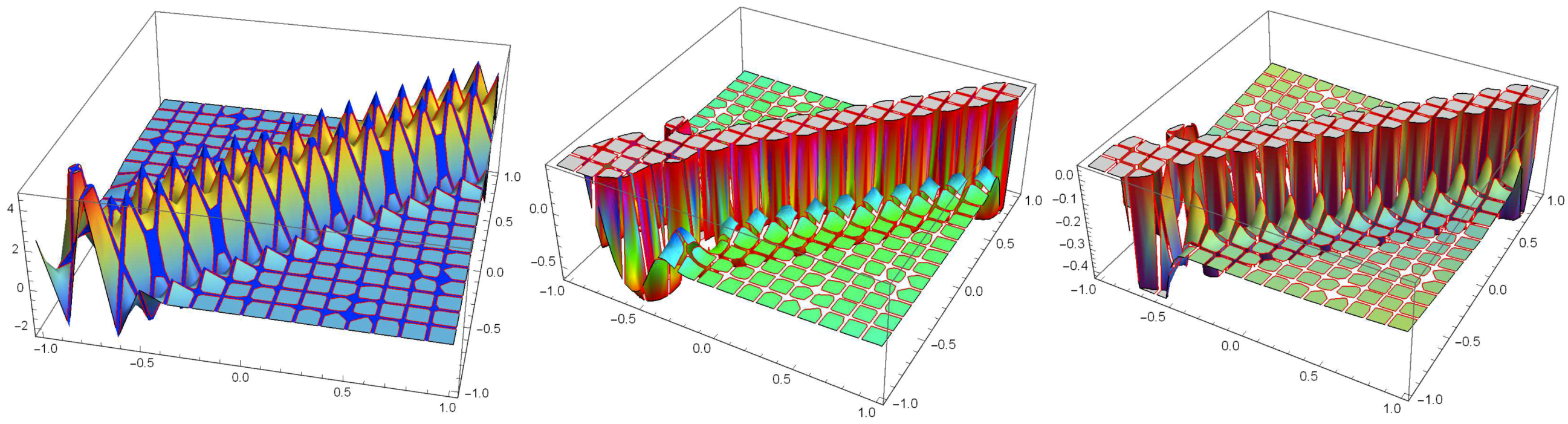
is called the kernel of ${\mathcal{Q}}_{n}f$. Figure 1 shows the graphs of the kernel ${\mathcal{D}}_2\left(x,y\right)$ for different framelets.

Figure 1. The graphs of the kernel, ${\mathcal{D}}_2(x,y)$, using the framelets of Example 2, 3 and 4, respectively.

It is known from the approximation theory, see e.g., Refs. ([28,35]), that the truncated expansion (7) is equivalent to

$${\mathcal{Q}}_{n}f=\sum _{k\in \mathbb{Z}}⟨f,{\tilde{\varphi }}_{n,k}⟩{\varphi }_{n,k},n\in {\mathbb{Z}}^{+},f\in L_2\left(\mathbb{R}\right).$$

(9)

The general setup is to construct a set of functions as the form of $\mathsf{\Psi }$, which can be summarized as follows: Let $V_0$ be the closed space generated by ${\left\{\varphi (·-k)\right\}}_{k\in \mathbb{Z}}$, i.e., $V_0=\overline{span}{\left\{\varphi (·-k)\right\}}_{k\in \mathbb{Z}}$, and $V_j=\left\{f\left(2^{j}x\right):f\left(x\right)\in V_0,x\in \mathbb{R}\right\}$. Let ${\left\{V_j,\varphi \right\}}_{j\in \mathbb{Z}}$ be the multiresolution analysis (MRA) generated by the function $\varphi$ and $\mathrm{\Psi }\subset V_1$ such that

$${\psi }^{\ell }=2\sum _{k\in \mathbb{Z}}{h}_{\ell }\left[k\right]\varphi (2·-k),$$

(10)

where ${\left\{h_{\ell }\left[k\right],k\in \mathbb{Z}\right\}}_{\ell =1}^r$ is a finitely supported sequence called high pass filters of the system. Please note that from Equation (7), the functions $\varphi ,{\psi }^{\ell }$ and $\tilde{\varphi },{\tilde{\psi }}^{\ell }$ are playing a great role. They are used for computing the coefficients of the expansion of the function f in terms of $\varphi$ and $\psi$, and recovering the projection of f onto $V_j$ from the coefficients $⟨f,{\tilde{\psi }}_{j,k}^{\ell }⟩$. The Fourier transform of a function $f\in L_2\left(\mathbb{R}\right)$ is defined to be

$$\mathcal{F}\left(f\right)\left(\omega \right)=\widehat{f}\left(\omega \right)={\int }_{\mathbb{R}}f\left(x\right)e^{-i\omega x}dx,\omega \in \mathbb{R},$$

and the Fourier series of a sequence $h\in {\ell }_2\left(\mathbb{Z}\right)$ is defined by

$$\mathcal{F}\left(h\right)\left(\omega \right)=\widehat{h}\left(\omega \right)=\sum _{k\in \mathbb{Z}}h\left[k\right]e^{-i\omega k},\omega \in \mathbb{R}.$$

2. Gibbs Effect in Quasi-Affine Dual Tight Framelet Expansions

In this section, we study the Gibbs effect by using dual tight framelet in the quasi-affine tight framelet expansions generated via the MOEP. In general, and by using the expansion in Equation (7), we have ${lim}_{n\to \infty }{\mathcal{Q}}_{n}f\left(x\right)=f\left(x\right)$ around x, where f is continuous except at many finite points. Hence, it is sufficient to study this effect by considering the following function

$$\begin{array}{c}\hfill f\left(x\right)=\left\{\begin{array}{cc}1-x,& 0<x\le 1\\ -1-x,& -1\le x<0\\ 0,& \mathrm{else}\end{array}\right..\end{array}$$

In fact, this function is useful in the sense that other functions that have the same type of gaps, can be represented as expansions in terms of f plus a continuous function at $x=0$. Please note that if we define $\mathcal{S}$ as

$$\begin{array}{c}\hfill \mathcal{S}\left(x\right)=\left\{\begin{array}{cc}\xi +1-x,& \xi <x\le \xi +1\\ \xi -1-x,& \xi -1\le x<\xi \\ 0,& \mathrm{else}\end{array}\right.,\end{array}$$

then, $\mathcal{S}$ has a jump discontinuity at the point $\xi$ and $\mathcal{S}\left(x\right)=f(x-\xi )$. Thus, we have the following result.

Theorem 1.

Any function with finitely many jump discontinuities can be written in terms of $\mathcal{S}$ plus a continuous function at the origin.

Proof. 

Let g be a discontinuous function with a jump discontinuity, say at $x=\xi$, of magnitude D. We could put several of these together for g but we would likely only be looking at one such function at a time. Suppose that $\mathcal{S}$ and g are in the same direction of the needed jump (i.e., if $g\left({\xi }^{+}\right)>g\left({\xi }^{-}\right)$, then $J\left({\xi }^{+}\right)>J\left({\xi }^{-}\right)$, and similarly for $g\left({\xi }^{+}\right)<g\left({\xi }^{-}\right)$) or multiply $\mathcal{S}$ by (− or +)D to create the needed jump in the same direction. Define

$$\begin{array}{c}\hfill F\left(x\right)=(+or-)D\mathcal{S}\left(x\right)+d,\end{array}$$

so that d is a constant that makes the jump endpoints of F and g matched at $x=\xi$. Our continuous function in the neighborhood of the point $\xi$ will then be $g\left(x\right)-F\left(x\right)$. □

The definition of the Gibbs effect under the quasi-projection approximation ${\mathcal{Q}}_n$ is defined as follows.

Definition 3.

Suppose a function f is smooth and continuous everywhere except at $x_{\circ }$, i.e., limits ${lim}_{x\to x_{\circ }^{+}}f\left(x\right)$ and ${lim}_{x\to x_{\circ }^{-}}f\left(x\right)$ exist, and that $f\left(x_{\circ }^{+}\right)$ & $\ne \&f\left(x_{\circ }^{-}\right)$. Define ${\mathcal{Q}}_{n}f$ to be the truncated partial sum of Equation (7). We say that the framelet expansion of f exhibits the Gibbs effect at the right-hand side of $x_{\circ }$ if there is a sequence $d_s>0$ converging to $x_{\circ }$, and

$$\underset{n,s\to \infty }{lim}{\mathcal{Q}}_{n}f\left(d_s\right)\left\{\begin{array}{cc}>f\left(x_{\circ }^{+}\right),& iff\left(x_{\circ }^{+}\right)>f\left(x_{\circ }^{-}\right)\\ <f\left(x_{\circ }^{+}\right),& iff\left(x_{\circ }^{+}\right)<f\left(x_{\circ }^{-}\right)\end{array}\right..$$

Similarly, we can define the Gibbs effect on the left-hand side of $x_{\circ }$.

Let $\mathsf{\Psi }$ to be the system defined by Definition 2. Thus, the corresponding quasi-affine system $X^J\left(\mathsf{\Psi }\right)$ generated by $\mathsf{\Psi }$ is defined by a collection of translations and dilation of the elements in $\mathsf{\Psi }$ such that

$$X^J\left(\mathsf{\Psi }\right)=\left\{{\psi }_{j,k}^{\ell }:1\le \ell \le r,j,k\in \mathbb{Z},\right\}$$

where

$${\psi }_{j,k}^{\ell }=\left\{\begin{array}{cc}{2}^{j/2}{\psi }^{\ell }(2^j·-k),& j\ge J\\ 2^j{\psi }^{\ell }(2^j·-2^{j}k)),& j<J\end{array}\right..$$

In the study of our expansion, we consider $J=0$. Many applications in framelet and approximation theory are modeled by non-negative functions. One family of such important functions are the B-splines, where the B-spline $B_m$ of order m is defined by

$$B_m=B_{m-1}\ast B_1={\int }_{(0,1]}{B}_{m-1}(·-x)dx$$

where

$$B_1={\chi }_{(0,1]}.$$

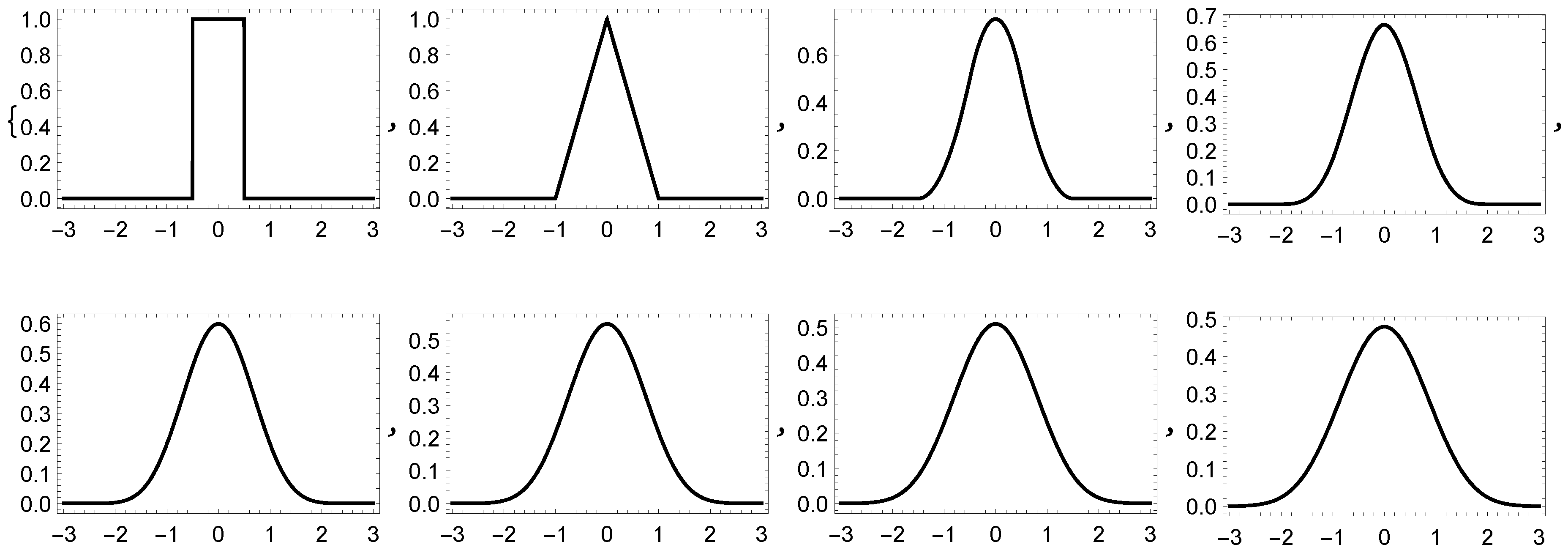
Figure 2 shows the graphs of the B-splines $B_m$ for different order.

Figure 2. B-splines of order 1 through 8, respectively.

It is known that sparsity of the framelets representations is due to the vanishing moments of the underling refinable wavelet (see Ref. [29]). We say $\psi$ has N vanishing moments if

$$\int x^r{\psi }_{j,k}^{\ell }\left(x\right)dx=0,forr=0,1,\cdots ,N-1,$$

(11)

which is equivalent to that ${\widehat{\psi }}_{j,k}^{\left(r\right)}\left(0\right)=0$, for all $r=0,1,\cdots ,N-1$. This implies that the framelet ${\psi }_{j,k}^{\ell }\left(x\right)$ is orthogonal to the polynomials $1,x,\cdots ,x^{N-1}$. The following statement is well known in the literature [13] for wavelets, but we present the proof for the reader’s convenience by considering the general quasi-affine dual framelet system.

Proposition 1.

Assume that $\tilde{\mathsf{\Psi }},\mathsf{\Psi }$ is a quasi-affine dual framelet system for $L_2\left(\mathbb{R}\right)$ and that ψ, where $\psi \in \mathsf{\Psi }$ has a vanishing moment of order N. Then for any polynomial $d\left(x\right)$ of degree at most $N-1$, we have

$$\mathcal{Q}d=d,$$

where $\mathcal{Q}={\mathcal{Q}}_0$ is defined by Equation (9) for $n=0$.

Proof. 

From the definition of $\tilde{\mathsf{\Psi }},\mathsf{\Psi }$, we know that all the generators must have a compact support. Therefore, we can find a positive integer A such that the support of all these generators lie in the interval $[-A,A]$. Define

$$C_B={\chi }_{[-B,B]},whereB\ge A.$$

(12)

Let $d(·)$ be a polynomial of degree at most $N-1$. Then, by the vanishing moment property of ${\psi }_{j,k}^{\ell }$ we have

$${\int }_{\mathbb{R}}{C}_{B}d\left(x\right){\psi }_{j,k}^{\ell }dx={\int }_{-B}^{B}d\left(x\right){\psi }_{j,k}^{\ell }dx=0,wherex<|B-A|.$$

(13)

Now, the proof is completed by taking $B\to \infty$ and using Equations (6) and (13). Thus, we have

$$d(·)=C_{B}d(·)=\sum _k⟨d,{\tilde{\varphi }}_{0,k}⟩{\varphi }_{0,k}(·)=\mathcal{Q}d(·).$$

 □

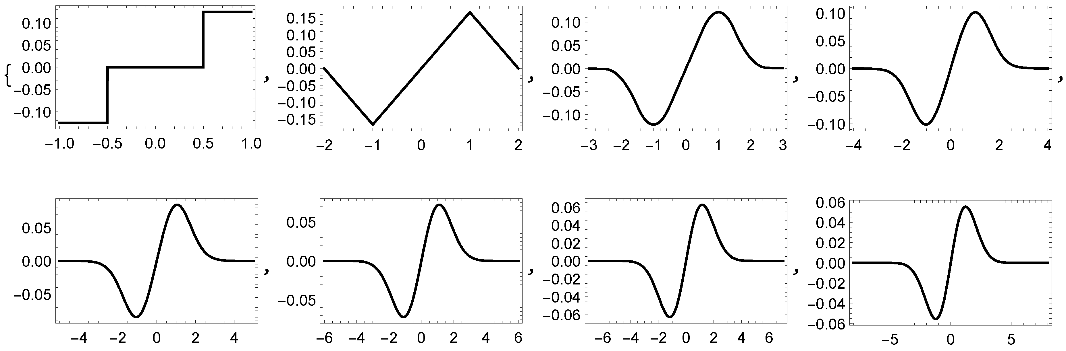
Now, we present some examples of dual tight framelets constructed by the MOEP in Ref. [34].

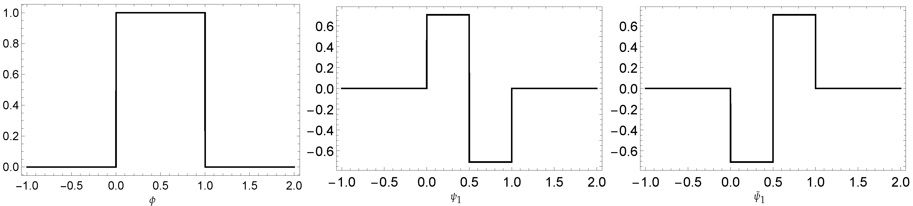
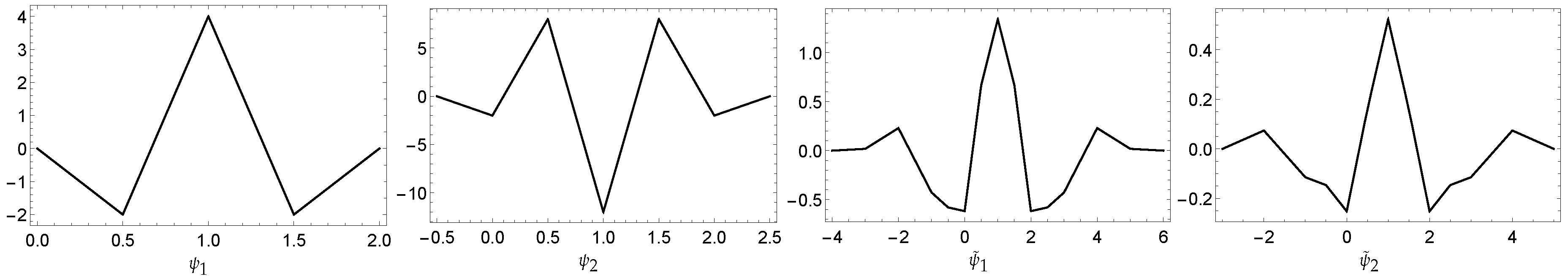
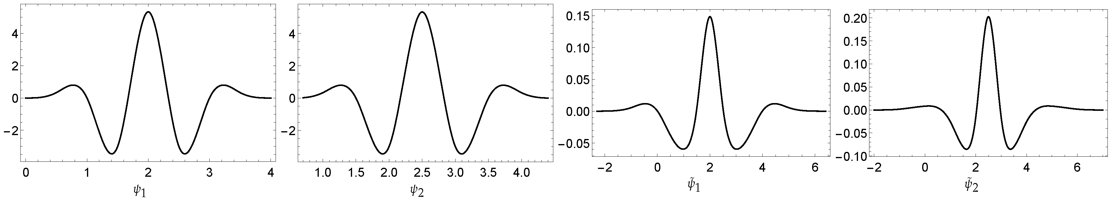
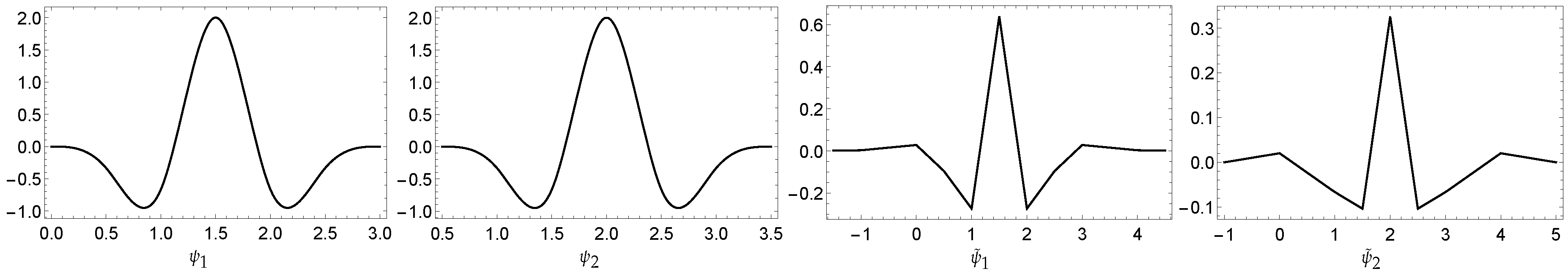
Example 1.

Let $B_1=\varphi ={\chi }_{[0,1)}$. Define,

$$\begin{array}{ccc}\hfill {\psi }_1\left(x\right)& =& \frac{529}{1497}{\chi }_{[0,1)}\left(2x\right)+\frac{-173}{489}{\chi }_{[0,1)}(2x-1),\hfill \\ \hfill {\tilde{\psi }}_1\left(x\right)& =& \frac{-1208}{3415}{\chi }_{[0,1)}\left(2x\right)+\frac{489}{1384}{\chi }_{[0,1)}(2x-1).\hfill \end{array}$$

Then, the resulting system generates a dual tight framelet for $L_2\left(\mathbf{R}\right)$. We illustrate the framelet and its dual framelet generators in Figure 3.

Figure 3. The graph of the Haar dual tight framelet of Example 1.

Example 2.

Let $B_2=\varphi =\tilde{\varphi }$. Then,

$$\mathcal{F}\left(h_0\right)\left(\xi \right)=\widehat{h_0}\left(\xi \right)=\widehat{{\tilde{h}}_0}\left(\xi \right)=0.25{(1+cos\left(\xi \right)-isin\left(\xi \right))}^2.$$

Thus, by using the MOEP, one can find the following high pass filters,

$$\begin{array}{ccc}\hfill {\widehat{h}}_1\left(\xi \right)& =& -{(1-cos\left(\xi \right)+isin\left(\xi \right))}^2,\hfill \\ \hfill {\widehat{h}}_2\left(\xi \right)& =& -16{sin}^4(\xi /2)(cos\left(\xi \right)-isin\left(\xi \right)),\hfill \\ \hfill {\widehat{\tilde{h}}}_1\left(\xi \right)& =& \frac{1}{480}{e}^{-i\xi }{sin}^4(\xi /2)(\mathrm{32,668}+\mathrm{57,569}cos\left(\xi \right)+\mathrm{39,422}cos\left(2\xi \right)+\mathrm{21,191}cos\left(3\xi \right)+\hfill \\ & & 8428cos\left(4\xi \right)+2233cos\left(5\xi \right)+426cos\left(6\xi \right)+71cos\left(7\xi \right)),\hfill \\ \hfill {\widehat{\tilde{h}}}_2\left(\xi \right)& =& -\frac{1}{480}{e}^{-i\xi }{sin}^2(\xi /2)(-614-726cos\left(\xi \right)+85cos\left(2\xi \right)+412cos\left(3\xi \right)+458cos\left(4\xi \right)\hfill \\ & & +284cos\left(5\xi \right)+71cos\left(6\xi \right)).\hfill \end{array}$$

Then, ${\psi }^{\ell },{\tilde{\psi }}^{\ell },\ell =1,2$ forms a dual tight framelets for $L_2\left(\mathbb{R}\right)$. These functions have vanishing moments (vm) as follows, $vm({\psi }_1)=vm({\tilde{\psi }}_2)=2$ while $vm({\psi }_2)=vm({\tilde{\psi }}_1)=4$. See Figure 4 for their graphs.

Figure 4. The graphs of the framelets and its dual framelets of Example 2.

Example 3.

Let $B_4=\varphi =\tilde{\varphi }$. Then,

$${\widehat{h}}_0\left(\xi \right)={\widehat{\tilde{h}}}_0\left(\xi \right)=0.0625{(1+cos\left(\xi \right)-isin\left(\xi \right))}^4.$$

We have the following high pass filters,

$$\begin{array}{ccc}\hfill {\widehat{h}}_1\left(\xi \right)& =& {(1-cos\left(\xi \right)+isin\left(\xi \right))}^4,\hfill \\ \hfill {\widehat{h}}_2\left(\xi \right)& =& 16{sin}^4(\xi /2)(cos\left(3\xi \right)-isin\left(3\xi \right)).\hfill \end{array}$$

The high pass filters for the dual framelets in ${\ell }_2\left(\mathbb{Z}\right)$, where $k\in \mathbb{Z}$, is given by

$$\begin{array}{c}\hfill \left\{\begin{array}{c}{\tilde{h}}_1\left[k\right]=[\frac{311}{\mathrm{3,870,720}},\frac{311}{\mathrm{967,680}},\frac{865}{\mathrm{387,072}},\frac{473}{\mathrm{64,512}},\frac{1783}{\mathrm{483,840}},\frac{-\mathrm{19,967}}{\mathrm{967,680}},\frac{-\mathrm{67,453}}{\mathrm{1,935,360}},\frac{-\mathrm{17,887}}{\mathrm{967,680}},\frac{\mathrm{233,473}}{\mathrm{1,935,360}},\frac{\mathrm{17,887}}{\mathrm{967,680}},\hfill \\ \frac{\mathrm{67,453}}{\mathrm{1,935,360}},\frac{\mathrm{19,967}}{\mathrm{967,680}},\frac{1783}{\mathrm{483,840}},\frac{473}{\mathrm{64,512}},\frac{865}{\mathrm{387,072}},\frac{311}{\mathrm{967,680}},\frac{311}{\mathrm{3,870,720}}],\hfill \\ {\tilde{h}}_2\left[k\right]=[\frac{311}{\mathrm{483,840}},\frac{311}{\mathrm{120,960}},\frac{2119}{\mathrm{483,840}},\frac{47}{\mathrm{10,080}},\frac{-4111}{\mathrm{483,840}},\frac{-5687}{\mathrm{120,960}},\frac{-\mathrm{21,103}}{\mathrm{483,840}},\frac{2627}{\mathrm{15,120}},\frac{-\mathrm{21,103}}{\mathrm{483,840}},\frac{-5687}{\mathrm{120,960}},\hfill \\ \frac{-4111}{\mathrm{483,840}},\frac{47}{\mathrm{10,080}},\frac{2119}{\mathrm{483,840}},\frac{311}{\mathrm{120,960}},\frac{311}{\mathrm{483,840}}].\hfill \end{array}\right.\end{array}$$

Then, ${\psi }^{\ell },{\tilde{\psi }}^{\ell },\ell =1,2$ forms a dual tight framelets for $L_2\left(\mathbb{R}\right)$. Here we have $vm({\psi }_1)=vm({\psi }_2)=vm({\tilde{\psi }}_1)=vm({\tilde{\psi }}_2)=4$. Their graphs are depicted in Figure 5.

Figure 5. The graphs of the framelets and its dual framelets of Example 3.

Example 4.

Let $B_4=\varphi$, and $B_2=\tilde{\varphi }$. Thus,

$${\widehat{h}}_0\left(\xi \right)=0.0625{(1+cos\left(\xi \right)-isin\left(\xi \right))}^4,and{\widehat{\tilde{h}}}_0\left(\xi \right)=0.25{(1+cos\left(\xi \right)-isin\left(\xi \right))}^2.$$

Then, we have the following tight framelets,

$${\psi }_1\left(x\right)=\left\{\begin{array}{cc}-8x^3/3\hfill & if0\le x\le 1/2\hfill \\ -2+12x-24x^2+40x^3/3\hfill & if1/2<x\le 1\hfill \\ 38-108x+96x^2-80x^3/3\hfill & if1<x<3/2\hfill \\ -142+252x-144x^2+80x^3/3\hfill & if3/2\le x<2\hfill \\ 178-228x+96x^2-40x^3/3\hfill & if2\le x<5/2\hfill \\ (8/3){(-3+x)}^3\hfill & if5/2\le x\le 3\hfill \\ 0\hfill & ifotherwise,\hfill \end{array}\right.$$

$${\psi }_2\left(x\right)=\left\{\begin{array}{cc}-(1/3){(-1+2x)}^3\hfill & if1/2\le x\le 1\hfill \\ -47/3+46x-44x^2+40x^3/3\hfill & if1<x<3/2\hfill \\ 358/3-224x+136x^2-80x^3/3\hfill & if3/2\le x<2\hfill \\ (2/3)(-461+624x-276x^2+40x^3)\hfill & if2\le x<5/2\hfill \\ 953/3-334x+116x^2-40x^3/3\hfill & if5/2\le x\le 3\hfill \\ (1/3){(-7+2x)}^3\hfill & if3<x\le 7/2\hfill \\ 0\hfill & ifotherwise\hfill \end{array}\right.$$

and the high pass filters for its dual tight framelets in ${\ell }_2\left(\mathbb{Z}\right)$, where $k\in \mathbb{Z}$, are given by:

$$\begin{array}{c}\hfill \left\{\begin{array}{c}{\tilde{h}}_1\left[k\right]=[\frac{13}{\mathrm{15,360}},\frac{13}{7680},\frac{61}{7680},\frac{109}{7680},\frac{-733}{\mathrm{15,360}},\frac{-35}{256},\frac{409}{1280},\frac{-35}{256},\frac{-733}{\mathrm{15,360}},\frac{109}{7680},\frac{61}{7680},\frac{13}{7680},\frac{13}{\mathrm{15,360}},],\hfill \\ {\tilde{h}}_2\left[k\right]=[\frac{13}{2560},\frac{13}{1280},\frac{-89}{7680},\frac{-1}{30},\frac{-199}{3840},\frac{313}{1920},\frac{-199}{3840},\frac{-1}{30},\frac{-89}{7680},\frac{13}{1280},\frac{13}{2560}].\hfill \end{array}\right.\end{array}$$

Then, again ${\psi }^{\ell },{\tilde{\psi }}^{\ell },\ell =1,2$ forms a dual tight framelets for $L_2\left(\mathbb{R}\right).$ Here we have $vm({\psi }_1)=vm({\psi }_2)=2,vm({\tilde{\psi }}_1)=vm({\tilde{\psi }}_2)=4$. Their graphs are depicted in Figure 6.

Figure 6. The graphs of the framelets and its dual framelets of Example 4.

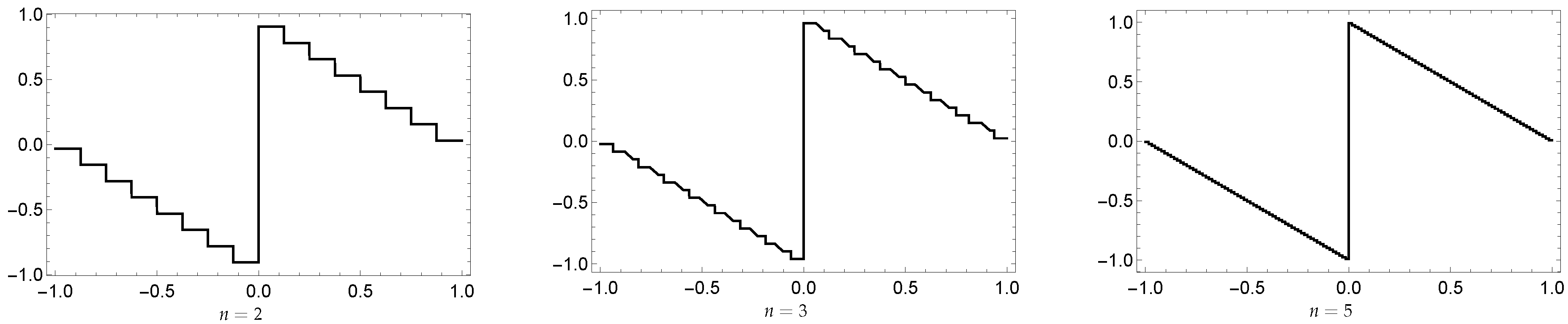
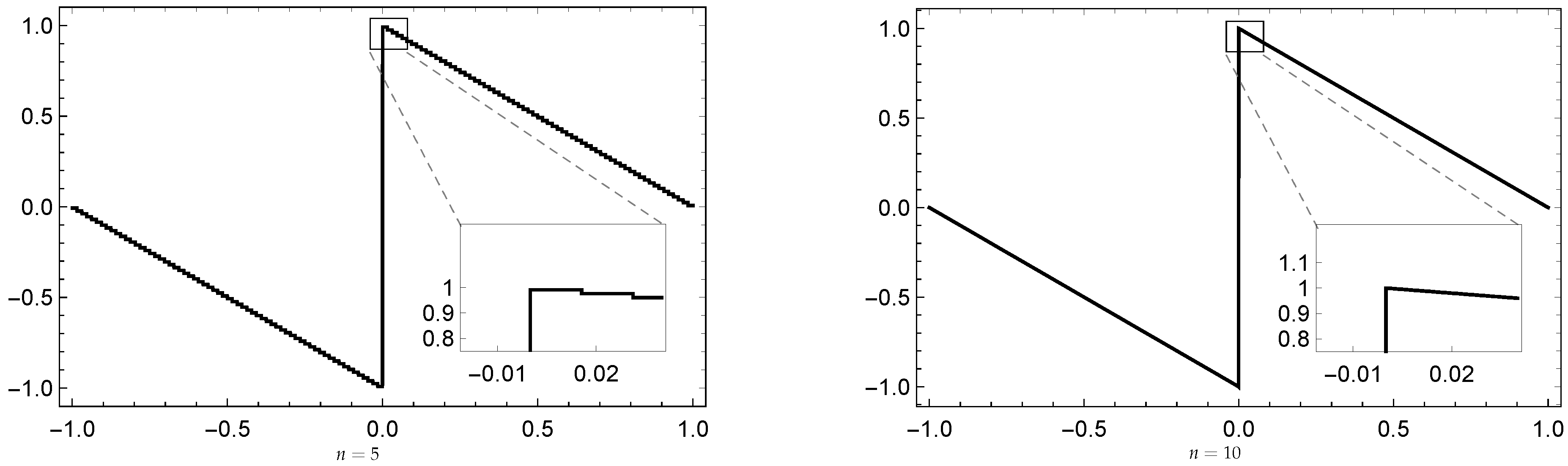
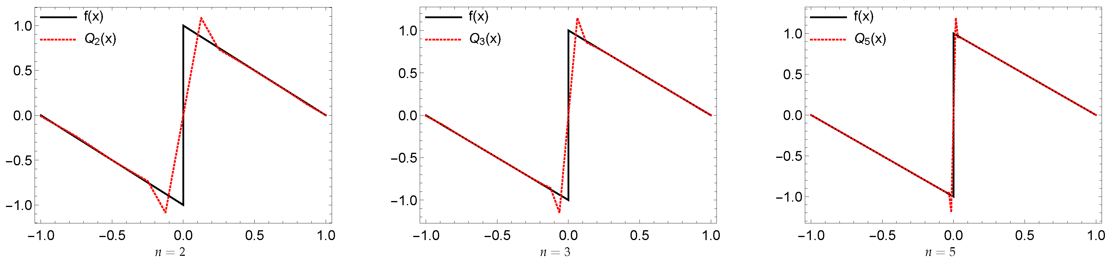
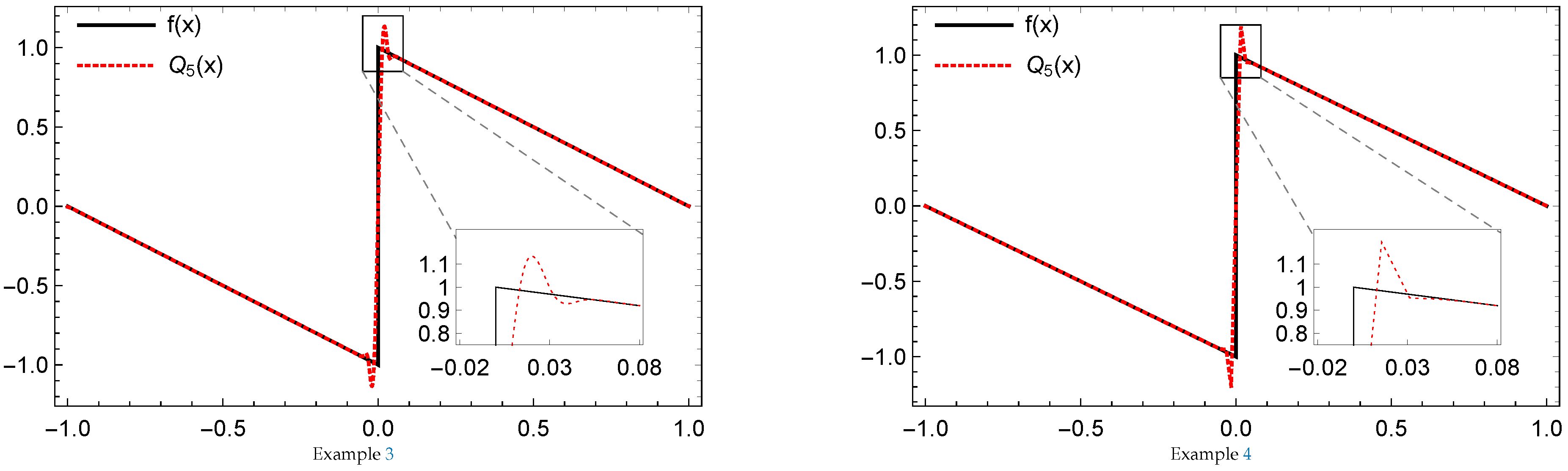
We will use the framelet expansion defined by Equation (7) to present the numerical evidence of the Gibbs effect by determining the maximal overshoot and undershoot of the truncated expansion ${\mathcal{Q}}_{n}f$ near the origin. The behavior of the truncated functions ${\mathcal{Q}}_n$ of a function with jump discontinuities is related to the existence of the Gibbs phenomenon, which is unpleasant in application, and not so easy to avoid. Therefore, examining a series of representations to avoid it or at least reduce it, is very important.

Proposition 2.

For any two refinable compactly supported functions ϕ and $\tilde{\varphi }$ in $L_2\left(\mathbb{R}\right)$. If

$$\mathcal{Q}sgn\le 1on(x_{\circ },\infty )and\mathcal{Q}sgn\ge -1on(-\infty ,x_{\circ }),$$

then ${\mathcal{Q}}_{n}f$ exhibits no Gibbs effect.

Proof. 

Please note that $\left({\mathcal{Q}}_{n}f\right)\left(2^{-n}x\right)=\mathcal{Q}\left(f\left(2^{-n}x\right)\right)$ for all $n\in \mathbb{N}$. In particular, $({\mathcal{Q}}_{n}sgn)\left(2^{-n}x\right)=\mathcal{Q}(sgn\left(2^{-n}x\right))$. Suppose that the truncated function ${\mathcal{Q}}_{n}f$ do exhibit the Gibbs effect near $x_{\circ }^{+}$. Thus, there exists an open interval $\mathcal{U}\subseteq (x_{\circ },\infty )$ such that $\mathcal{Q}f\left(x\right)>1,\forall x\in \mathcal{U}$. Therefore, $\exists u>x_{\circ }$ such that ${max}_{x\in (x_{\circ },u)}\mathcal{Q}f\left(x\right)=U>1$. Define a sequence $u_n>x_{\circ },\forall n$ such that $u_n\to x_{\circ }$ as $n\to \infty$ (one can take $u_n={ϵ}_n+x_{\circ }$ such that ${ϵ}_n\to 0$ as $n\to \infty$). Hence, ${max}_{x\in (x_{\circ },u_n)}{\mathcal{Q}}_{n}f\left(x\right)={max}_{x\in (x_{\circ },u)}\mathcal{Q}f\left(x\right)=U>1$, a contradiction. Similarly, we can prove the case when $x<x_{\circ }^{-}$ in the same fashion. □

Please note that it is important to use non-negative functions in framelet analysis due to its use in a variety of applications. One of those functions is the B-splines. The following statement will require such non-negativity to avoid the Gibbs effect.

Theorem 2.

Let ϕ and $\tilde{\varphi }$ be any two non-negative refinable real valued compactly supported functions in $L_2\left(\mathbb{R}\right)$ such that

$$\int sgn\left(x\right)\varphi (x-k)>0and\int sgn\left(x\right)\tilde{\varphi }(x-k)>0on\mathbb{R}.$$

Assume further ${\sum }_k\varphi (x-k)=1$. If the vanishing moment of ϕ and $\tilde{\varphi }$ is one, then $\tilde{\mathcal{Q}}f$ exhibit no Gibbs effect.

Proof. 

It suffices to show this for $sgn\left(x\right)$ as $f\left(x\right)=sgn\left(x\right)-x$ on $[-1,1]$. Please note that Proposition 1 is held for $d=1$, i.e.,

$$\tilde{Q}1=1.$$

Now, for $x\in \mathbb{R}$, and since

$$⟨sgn\left(x\right),\varphi (x-k)⟩=\widehat{\varphi }\left(0\right),$$

by assumption, we have

$$\begin{array}{ccc}\hfill \tilde{\mathcal{Q}}sgn\left(x\right)-1& =& \sum _k⟨sgn\left(x\right),\varphi (x-k)⟩\tilde{\varphi }(x-k)\hfill \\ & =& -\sum _k\left({\int }_{-\infty }^{-k}\varphi \left(x\right)dx\right)\tilde{\varphi }(x-k)<0.\hfill \end{array}$$

The other side is analogue. Thus, $-1\le \tilde{\mathcal{Q}}sgn\le 1$ for all $x\in \mathbb{R}$. □

3. Results and Discussion

We present some numerical illustration by using the dual tight framelets which will generalize the result in Ref. [14]. The results show that if the dual framelet has vanishing moments of order of at least two, then ${\mathcal{Q}}_{n}f$ must exhibit the Gibbs effect. However, ${\mathcal{Q}}_{n}f$ has no Gibbs effect by using dual tight framelets of vanishing moments of order one.

Now we present an illustration for the Gibbs effect using the above dual tight framelets by showing the maximum overshoots, undershoots of $f\left(x\right)$, and some related graphs. This is to showcase the absence of the effect in Table 1 and Figure 7 and Figure 8.

Table 1. Approximate maximum overshoot and undershoot in neighborhoods of $x=0$ using ${\mathcal{Q}}_{n}f$ of Example 1.

Level	Maximum	Minimum
$n=2$	$0.907276$	$-0.907276$
$n=3$	$0.964562$	$-0.964562$
$n=5$	$0.994801$	$-0.994802$
$n=10$	$0.999968$	$-0.999972$

Figure 7. Illustration for the absence of the Gibbs effect using the quasi-operator ${\mathcal{Q}}_{n}f$ of Example 1.

Figure 8. Illustration for the absence of the Gibbs effect using the quasi-operator ${\mathcal{Q}}_{n}f$ of Example 1 for $n=5,10$, respectively.

In Figure 9 and Figure 10 we illustrate the graphs of the function $\mathcal{Q}f$ and $\mathcal{Q}sgn$, receptively, generated using the B-splines dual tight framelets. In Table 2, Table 3 and Table 4 we show the approximated values for the overshoots and undershoots of ${\mathcal{Q}}_{n}f$. Figure 11, Figure 12, Figure 13 and Figure 14 illustrate the graphs of the Gibbs effect.

Figure 9. Graphs of $\mathcal{Q}f\left(x\right)$ by the B-splines of order 1 through 8, respectively.

Figure 10. Graphs of $\mathcal{Q}sgn\left(x\right)$ by the B-splines of order 1 through 8, respectively.

Table 2. Approximate maximum overshoot and undershoot in neighborhoods of $x=0$ using ${\mathcal{Q}}_{n}f$ of Example 2 for $n=2,3,5,10$.

Level	Maximum	Minimum
$n=2$	$1.0021$	$-1.01204$
$n=3$	$1.12708$	$-1.12708$
$n=5$	$1.22083$	$-1.18958$
$n=10$	$1.25111$	$-1.25111$

Table 3. Approximate maximum overshoot and undershoot in neighborhoods of $x=0$ using ${\mathcal{Q}}_{n}f$ of Example 3 for $n=2,3,5,10$.

Level	Maximum	Minimum
$n=2$	$0.997622$	$-0.996194$
$n=3$	$1.07451$	$-1.07451$
$n=5$	$1.13384$	$-1.13384$
$n=10$	$1.15337$	$-1.15337$

Table 4. Approximate maximum overshoot and undershoot in neighborhoods of $x=0$ using ${\mathcal{Q}}_{n}f$ of Example 4 for $n=2,3,5,10$.

Level	Maximum	Minimum
$n=2$	$1.08519$	$-1.08526$
$n=3$	$1.14823$	$-1.14823$
$n=5$	$1.19514$	$-1.19514$
$n=10$	$1.21028$	$-1.21028$

Figure 11. Illustration of the Gibbs effect using the quasi-operator ${\mathcal{Q}}_{n}f$ of Example 2.

Figure 12. Illustration of the Gibbs effect using the quasi-operator ${\mathcal{Q}}_{n}f$ of Example 3.

Figure 13. Illustration of the Gibbs effect using the quasi-operator ${\mathcal{Q}}_{n}f$ of Example 4.

Figure 14. Gibbs effect illustrations by ${\mathcal{Q}}_{5}f\left(x\right)$ of Example 3 and 4, respectively.

4. Conclusions

According to the above results, we show that the Gibbs effect is absent when the dual tight framelets of vanishing moments of order one are used to represent a function with jump discontinuities at the origin. Please note that increasing the vanishing moments, e.g., using the MOEP, will increase the approximation order of the framelet representation ${\mathcal{Q}}_{n}f$ that used to expand the function f; however, the Gibbs effects cannot be avoided for any level of n. Quite a few examples of dual tight framelets, numerical results, and graphical illustrations have been presented for the absence and presence of Gibbs effect.