Natural Test for Random Numbers Generator Based on Exponential Distribution

Abstract

We will prove that when uniformly distributed random numbers are sorted by value, their successive differences are a exponentially distributed random variable Ex(λ). For a set of n random numbers, the parameters of mathematical expectation and standard deviation is λ = n⁻¹. The theorem was verified on four series of 200 sets of 101 random numbers each. The first series was obtained on the basis of decimals of the constant e = 2.718281…, the second on the decimals of the constant π = 3.141592…, the third on a Pseudo Random Number generated from Excel function RAND, and the fourth series of True Random Number generated from atmospheric noise. The obtained results confirm the application of the derived theorem in practice.

1. Introduction

Random numbers generators are applicable in various areas, such as: Computer simulation, Monte-Carlo method, multiple integration, nonconvex global optimization, scientific computing, commercial finance, electronic gambling equipment (including on-line gambling), and other fields. The modern world ’exploits’ a huge amount of random numbers. Especially in the field of information security, which is based on the cryptography where encryption key randomness is essential [1,2], the quality of random numbers is directly related to the secure transmission of information [3].

One of the basic functions of the human brain is the ability to generate random numbers [4,5]. There are significant differences in activities of particular brain centers during the processes of generating ordinal numbers and random numbers. The inability of a person to generate random numbers may indicate possible disorders. Furthermore, distinctions in brain functions while generating random numbers may significantly imply certain diseases: Dementia of the Alzheimer type, schizophrenia, multiple sclerosis, and Parkinson’s disease [6,7,8,9]. Nonetheless, the human brain as the natural source of random numbers does not represent a significant quantitative capacity. The ability to mimic natural entropy is obviously an extremely intellectual demand. However, materialized mental models with computers completely eliminate this deficit.

Random sequences are produced by two basic types of generators: The True or Physical Random Number Generator (TRNG) and the Pseudo-Random Number Generator (PRNG). True or physical random numbers are generated by a stochastic physical entropy source in the natural world, such as radioactive decay, thermal noise in resistors, the frequency jitter in an oscillator, single photon splitting on a beam-splitter, amplified spontaneous emissions, chaotic laser, and so on [9]. The natural source of TRNGs is number π [10,11]. TRNGs usually need some post-processing functions for producing random sequences in physical quantities. Everyday life requires converting physical quantities into digital ones. The generation of random numbers in total meets the demand [12]. The quality of a PRNG is defined as the randomness of its outputs, whereby high-quality, cryptographically strong PRNGs are practically indistinguishable from TRNG [13].

Generating pseudo-random numbers by using computers is a fast and cheap way to provide substantial quantities. Pseudo-random numbers generated in that way must comply with the following criteria: A certain sequence length without repetition, uniformity, and resolution, etc., [14]. For generating pseudo-random numbers, a large number of PRNGs is used, as well as a large number of tests which must verify the randomness of generated numbers [15,16,17,18,19,20], i.e., quality of the random number generator. Diehard contains 12 tests, with confirmation that the generators that pass the three tests (GCD-greatest common divisor, The Gorilla Test, and The Birthday Spacings Test) seem to pass all the tests in the Diehard Battery of Tests [21]. TESTU01 offers three batteries of tests called ‘Small Crush’ (which consists of 10 tests), ‘Crush’ (60 tests), and ‘Big Crush’ (45 tests) [22]. The NIST battery contains 15 tests: The Frequency (Monobit) Test, The Discrete Fourier Transform (Spectral) Test, Maurer’s “Universal Statistical” Test, The Approximate Entropy Test, Cusums Test, etc., [23]. The reference distributions of tests are dominated by Normal, half-Normal, andχ² distributions. In accordance with the CLT—Central Limit Theorem—, this outcome is partially expected. However, The Birthday Spacings Test from the Diehard Battery is asymptotically exponentially distributed. The first question is: Why does the Birthday Spacings Test have a hard-shell against the CLT attitude?

According to the de Moivre-Laplace theorem (the earliest version of CLT), the Binomial distribution of binary sequences (the original input string of zero and one to be tested) has a Normal distribution. Now, another question arises: If χ² is the reference distribution in 10 of the 15 NIST tests, then why the Normal distribution not prevalent?

On the other hand, the Binomial distribution B(p, n) can be approximated by the Poisson distribution P(λ), np = λ. Exponential distribution with parameter λ is the basis of Poison’s processes with the identical parameter λ. Thus, the Binomial distribution of binary sequences can be approximated by an Exponential distribution, Ex(np).

An important property of a set of random numbers is a complete mutual independence of the previous and subsequent generated digits. Such a “longitudinal” lack of influence or unpredictability is the known property of exponential distribution (1):

$$f(t;\lambda )=\{\begin{array}{cc}\lambda e^{-\lambda t},& t\ge 0\\ 0,& t<0\end{array},F(t;\lambda )=\{\begin{array}{cc}1-e^{-\lambda t},& t\ge 0\\ 0,& t<0\end{array}$$

(1)

described with memoryless properties (2):

$$P\left(\raisebox{1ex}{$T>a+b$}\!\left/ \!\raisebox{-1ex}{$T>a$}\right.\right)=\frac{P(T>a+b)}{P(T>a)}=\frac{{\displaystyle \underset{a+b}{\overset{\infty }{\int }}\lambda e^{-\lambda t}dt}}{{\displaystyle \underset{a}{\overset{\infty }{\int }}\lambda e^{-\lambda t}dt}}=\frac{e^{-\lambda (a+b)}}{e^{-\lambda a}}={\displaystyle \underset{b}{\overset{\infty }{\int }}\lambda e^{-\lambda t}dt}=P(T>b).$$

(2)

In the class of random variables whose densities are positive at [0, ∞) and with an equal expectation, the highest differential entropy has an exact exponential distribution.

Wide use of exponential distribution has long been known in natural and technical processes [24,25,26,27,28]. The recognition period of significance of exponential distribution corresponds with the occurrence of first tests of random numbers [29]. An analogy of the natural entropy and differential entropy of information theory points to potential of exponential distribution. Furthermore, if we adopt the difference between stochasticity and randomness [30] or, respectively, TRNG/PRNG, then the application of Poisson processes in randomness testing, the essential relation between the Poisson and exponential distribution and the maximal differential entropy of exponential distribution, spontaneously forms an idea of the application of a memoryless characteristic (2) in the testing of random numbers. The next theorem proves the existence of these two stated ideas.

2. Exponential Distribution of the Successive Difference Between Random Numbers

Let us denote by T_i−1 the interval between two random adjacent events {t_i−1, t_i} in the stream of the independent events {t₁, t₂, t₃, …, t_n, t_n+1} in which the event S has been realized by the random selection of intervals (Figure 1):

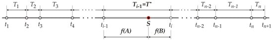
Figure 1. Stream of the independent events t_i, intervals T_i, and the independent choice of an interval T^•.

Theorem 1.

If the random events {t₁, t₂, t₃, …, t_n, t_n+1} are independent and uniformly distributed on the arbitrary interval, arranged so that ∀i∈[1, n], t_i ≤ t_i+1, then the intervals between the successive random events T_i−1 = (t_i − t_i−1) are such that ∀i∈[1, n], t_i ≤ t_i+1 has the exponential distribution with the values of mathematical expectation and standard deviation reciprocal to the number of random events n.

Proof. 

The procedure of proving the Theorem will be derived by mathematical induction. For this purpose, we need to find the first, second, and third moment of the distribution of intervals between the successive random events T_i−1.

Let the distribution function and the density distribution of the random variable T be equal to F(T) if (T) = F′(T). We need to find the density f(T^•) of the interval T, that is, the point S randomly distributed in the intervals A and B.

Random variables T and T^•, do not have the same functions and density distributions, f(T) ≠ f(T^•) and F(T) ≠ F(T^•). The probability of an arbitrary choice of the interval from the point S is proportional to the length of the interval. In a greater number of repetitions, the point S will more often fall on the longer intervals than on the shorter ones. Therefore, we can conclude that the choice probability of the interval T^• is higher than the average choice probability of the interval E(T) ≤ E(T^•).

The density distribution of the event T^• in the interval (t_i−1, t_i) is equal to f(T^•)dT. If n intervals are defined, then the average number of intervals is equal to n⋅f(t)dt, and the average length of all intervals is equal to t⋅n⋅f(t)dt. If the average f(T) is equal to E(T), then the average length of all n intervals is equal to n⋅E(T). Probability f(T^•)dT is approximately equal to the ratio between the sum of intervals with the length between t_i−1 and t_i and the total length of all intervals between the moments of the event appearance. This approximate equality is more accurate if the interval (t_i−1, t_i) is longer and the number of intervals greater. The density of the random variable T^• is equal to (3) [31]:

$$f(T^{•})dT\approx \frac{n\cdot T\cdot f(T)dT}{n\cdot E(T)}=\frac{T}{E(T)}f(T)dT,f(T^{•})=\{\begin{array}{cc}\frac{1}{E(T)}f(T),& T>0\\ 0,& T<0\end{array}.$$

(3)

In order to determine the mathematical expectation and variance of the random variable T^• it is necessary to determine the characteristic function of the random variable T (4):

$$k_T(x)=E(e^{ixT})={\displaystyle \underset{-\infty }{\overset{+\infty }{\int }}{e}^{ixT}f(t)dt}$$

(4)

Since $E(T^r)=\frac{k_T^{(r)}(0)}{i^r}$, the E(T) and V(T) of the random variable T are equal to (5):

$$E(T)=-{k^{\prime }}_T(0);E(T^2)=-{k^{″}}_T(0);V(T)=-{k^{″}}_T(0)+{[-{k^{\prime }}_T(0)]}^2.$$

(5)

The characteristic function of the random variable T^• is equal to (6):

$$k_{T^{•}}(x)={\displaystyle \underset{-\infty }{\overset{+\infty }{\int }}{e}^{ixt}f(T^{•})dT}={\displaystyle \underset{-\infty }{\overset{+\infty }{\int }}{e}^{ixt}\frac{t}{E(T)}f(T)dT}.$$

(6)

Since $T{e}^{Txt}=-i\frac{\partial }{\partial x}{e}^{ixT}$, it follows that (7):

$$k_{T^{•}}(x)=-i\frac{\partial }{\partial x}{\displaystyle \underset{-\infty }{\overset{+\infty }{\int }}{e}^{ixt}\frac{1}{E(T)}f(t)dt}=\frac{{k^{\prime }}_T(x)}{iE(T)}=\frac{{k^{\prime }}_T(x)}{{k^{\prime }}_T(0)}$$

(7)

So that the average value is equal to (8):

$$E(T^{•})=\frac{{k^{\prime }}_{T^{•}}(0)}{i}=\frac{{k^{″}}_{T^{•}}(0)}{i{k^{\prime }}_{T^{•}}(0)}=-\frac{E(T^2)}{i^{2}E(T)}=\frac{E(T^2)}{E(T)}=\frac{E{(T)}^2+D(t)}{E(T)}=E(T)+\frac{V(T)}{E(T)}$$

(8)

Since (9)

$${k^{″}}_{T^{•}}(x)=\frac{{k^{‴}}_T(x)}{iE(T)}\iff {k^{″}}_{T^{•}}(0)=\frac{{k^{‴}}_T(0)}{iE(T)}=-\frac{iE(T^3)}{iE(T)},$$

(9)

The variance of the random variable T^• is (10):

$$V(T^{•})=-{k^{″}}_T(0)+{[{k^{\prime }}_{T^{•}}(0)]}^2=\frac{E(T^3)}{E(T)}-\frac{{[E(T^2)]}^2}{E{(T)}^2}.$$

(10)

If we divide the interval T^•, whose event S has been implemented, into two intervals A and B, so that

→	• The interval A is equal from the previous event ti−1 to the event S
→	• The interval B is equal from the event S to the following event ti.

The density of the random variable B on the interval T^• equals:

$$f(T^{•},B)=f(T^{•})\varphi (B/T^{•}).$$

Due to stationarity, it applies (11):

$$\varphi (B/T^{•})=\{\begin{array}{cc}\frac{1}{T^{•}},& B\in (0,T^{•})\\ 0,& B\notin (0,T^{•})\end{array}\iff \varphi (B)={\displaystyle \underset{-\infty }{\overset{\infty }{\int }}f(T^{•},B)d{T}^{•}}={\displaystyle \underset{-\infty }{\overset{\infty }{\int }}{f}^{•}(T^{•})\varphi (B/T^{•})d{T}^{•}}.$$

(11)

Subintegral function is greater than zero only for values $T^{•}>B$, so we get (12):

$$\varphi (B)={\displaystyle \underset{S}{\overset{\infty }{\int }}\frac{T^{•}}{E(T)}}f(T^{•})\frac{1}{T^{•}}d{T}^{•}=\frac{1-F(B)}{E(T)}$$

(12)

where F(T) is distribution function of the random variable T, i.e., $F(T)={\displaystyle \underset{0}{\overset{T}{\int }}f(T)dT}$. Thus, the density of a probability distribution for the rest of the variable B from the random point S to the next event is (13):

$$\varphi (B)=\{\begin{array}{cc}\frac{1-F(B)}{E(T)},& B>0\\ 0,& B<0\end{array}.$$

(13)

The characteristic function of the random variable B equals (14):

$$k_B(x)={\displaystyle \underset{0}{\overset{\infty }{\int }}{e}^{ixB}\varphi (B)dB}=\frac{1}{E(T)}{\displaystyle \underset{0}{\overset{\infty }{\int }}{e}^{ixB}[1-F(B)]dB}.$$

(14)

Using the partial integration, we get (15):

$$k_B(x)=\frac{1}{E(T)}\left\{{[1-F(x)]\frac{e^{ixB}}{ix}|}_0^{\infty }+{\displaystyle \underset{0}{\overset{\infty }{\int }}\frac{e^{ixB}}{ix}f(B)dB}\right\}=\frac{k_T(x)-1}{ixE(T)}=\frac{k_T(x)-k_T(0)}{x{k^{\prime }}_T(0)}.$$

(15)

The mathematical expectation of the random variable B equals (16):

$$E(B)=\frac{1}{i^{2}E(T)}{\left\{\frac{\partial }{\partial x}\left[\frac{k_T(x)-1}{x}\right]\right\}}_{x=0}=-\frac{1}{E(T)}{\left\{\frac{{k^{\prime }}_T(x)\cdot x-k_T(x)+1}{x^2}\right\}}_{x=0}.$$

(16)

Since for x = 0 we get the vagueness in the form of “0/0”, thus by applying L’Hopital’s rule we get (17) [31]:

$$E(B)=-\frac{{k^{″}}_T(0)}{2E(T)}=\frac{V(T)+E{(T)}^2}{2E(T)}=\frac{1}{2}\left[E(T)+\frac{V(T)}{E(T)}\right]=\frac{E(T^{•})}{2}.$$

(17)

Using the connection ${k^{″}}_B(0)=-\frac{E(T^3)}{3E(T)}$ for variance of the random variable B, we get (18):

$$V(B)=-{k^{″}}_B(0)+{\left[{k^{\prime }}_B(0)\right]}^2=\frac{E(T^3)}{3E(T)}-\frac{{[E(T^2)]}^2}{4E^2(T)}.$$

(18)

The same applies for the random variable A (19):

$$E(A)=\frac{E(T^{•})}{2},V(A)=-{k^{″}}_A(0)+{\left[{k^{\prime }}_A(0)\right]}^2=\frac{E(T^3)}{3E(T)}-\frac{{[E(T^2)]}^2}{4E^2(T)}.$$

(19)

The density of distribution for the random variables A and B are identical. Provided that the characteristics of the uniform distribution of random events have not changed, the probability distributions T, A, and B are identical. From (17), (18), and (19) we get (20) and (21):

$$E(A)=E(B)=E(T)=\frac{E(T^{•})}{2}=\frac{E^2(T)+V(T)}{2E(T)}$$

(20)

$$V(A)=V(B)=V(T)=\frac{E(T^3)}{3E(T)}-\frac{{[E(T^2)]}^2}{4E^2(T)}$$

(21)

The uniformity requirement enables us to form a system of equations with the solutions (22):

$$E(T)=\frac{E^2(T)+V(T)}{2E(T)}=\frac{E^2(T)+E(T^2)-E^2(T)}{2E(T)}\iff E(T^2)=2E^2(T).$$

(22)

When we introduce the obtained relationship from Equations (20) and (21), we get (23):

$$V(T)=E(T^2)-E^2(T)=\frac{E(T^3)}{3E(T)}-\frac{{[E(T^2)]}^2}{4E^2(T)}\iff E(T^2)-E^2(T)=\frac{E(T^3)}{3E(T)}-\frac{{[2E^2(T)]}^2}{4E^2(T)}.$$

(23)

The expression for $E(T^3)$ from (22) and (23) is (24):

$$E(T^2)-E^2(T)=\frac{E(T^3)}{3E(T)}-E^2(T)\iff E(T^2)=2E^2(T)=\frac{E(T^3)}{3E(T)}\iff 6E^3(T)=E(T^3).$$

(24)

By mathematical induction we establish for k = 1, k = 2 and k = 3. The basic conditions of the division of n intervals, from (6), imply mathematical expectation for k = 1 as (25):

$${\displaystyle \sum _{i=1}^n{T}_i^{k}P(T_i)}={\displaystyle \sum _{i=1}^n{T}_i^{1}P(T_i)}=E(T^1)=1E^1(T)=1!E^1(T)=\frac{1}{n}.$$

(25)

From (22), it follows that for k = 2 (26):

$${\displaystyle \sum _{i=1}^n{T}_i^{k}P(T_i)}={\displaystyle \sum _{i=1}^n{T}_i^{2}P(T_i)}=E(T^2)=2E^2(T)=2!E^2(T)=\frac{1\cdot 2}{n^2}.$$

(26)

From (24), it follows that for k = 3 (27):

$${\displaystyle \sum _{i=1}^n{T}_i^{k}P(T_i)}={\displaystyle \sum _{i=1}^n{T}_i^{3}P(T_i)}=E(T^3)=6E^3(T)=3!E^3(T)=\frac{1\cdot 2\cdot 3}{n^3}.$$

(27)

Let us assume that for the integer k is fulfilled (28):

$${\mathsf{\Lambda }}_k={\displaystyle \sum _{i=1}^n{T}_i^{k}P(T_i)}=E(T^k)=k!E^k(T)=\frac{k!}{n^k}.$$

(28)

With the assumption for k, for (k+1) it follows (29):

$${\displaystyle \sum _{i=1}^n{T}_i^{k+1}P(T_i)}=E(T^{k+1})=(k+1)!E^{k+1}(T)=\left[(k+1)E(T)\right]k!E^k(T)=\frac{(k+1)!}{n^{k+1}}.$$

(29)

This proves that for every integer ∀n∈N, it is valid (30):

$${\displaystyle \sum _{i=1}^n{T}_i^{k+1}P(T_i)}=\left[(k+1)E(T)\right]{\displaystyle \sum _{i=1}^n{T}_i^{k}P(T_i)}=\frac{k!}{n^k}.$$

(30)

The distribution of a random variable T_i is exponential because the ratio of moments of the exponential distribution is equal to $E(T^k)=k!E^k(T)$. The condition results in the following: The variance and the standard deviation of the distribution of the random variable T is equal to (31):

$$V(T)={\displaystyle \sum _{i=1}^n{T}_i^3}-\frac{1}{n^2}={\displaystyle \sum _{i=1}^n{T}_i^2}P(T_i)-\frac{1}{n^2}=\frac{2!}{n^2}-\frac{1}{n^2}=\frac{1}{n^2}\iff \sigma (T)=\sqrt{V(T)}=\frac{1}{n}=E(T)$$

(31)

These are the identifiable parameters of the exponential distribution (Figure 2).

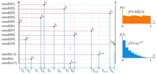
Figure 2. Fundamental concept is based on the theorem proof.

Random events {t₁, t₂, t₃, …, t_n, t_n+1} are independent. Distribution interval {T₁, T₂, …, T_n} between successive values of the random events {t₁, t₂, t₃, …, t_n, t_n+1} is exponential. Independence of random events {t₁, t₂, t₃, …, t_n, t_n+1} comes directly from (2)—the memoryless of the exponential distribution.

3. Application of Theorem

Pursuant to the theorem proof, successive differences {T₁, T₂, …, T_n} of n independent random numbers {t₁, t₂, t₃, …, t_n, t_n+1} have an exponential distribution with mathematical expectation and function of distribution density (32):

$$E(T)=\frac{1}{\lambda }=\frac{1}{n}\iff \lambda =n,f(T)=n{e}^{-nT}.$$

(32)

Four series of random numbers were prepared for testing. The first series is formed by successive decimals of the constant e = 2.718281…, the second series is formed by successive decimals of the constant π = 3.141592… The third series of Pseudo Random Numbers, PRNG was generated from Microsoft Excel’s RAND function. The fourth series of True Random Numbers, TRNG was generated from atmospheric noise [32]. Table 1 contains a series of these numbers.

Table 1. Series of random numbers.

“e” decimals	271828182845904523536028747135266249775724709369995957496696762772407663035354759457138217852516642742746639193200305992181741359662904357290033429526059563073813232862794349076323382988075319525101901157383418793070215408914993488416750924476146066808226480016847741185374234544243710753907774499206955…
“π” decimals	314159265358979323846264338327950288419716939937510582097494459230781640628620899862803482534211706798214808651328230664709384460955058223172535940812848111745028410270193852110555964462294895493038196442881097566593344612847564823378678316527120190914564856692346034861045432664821339360726024914127372…
PRNG	7259227051902899760820653695717034400802758150121933828161585021229157597171018544683160397426233882495837244083781905313129529407819631027568084023355456995655961036454261291377117301740011443026315431314350950726053529878643963583104666483673482473576217179604102739202744182506031608391653276202184739…
TRNG	5702321834924319698039224328949632170253798713293486165903367803756808794325594419963116773060031715966487336963199719730183382190863756390073297420987570798457304675443797726780701009434479393354064614498365777658458194195989924883287287212182011407782292143460981825932571746610515092283157440087522747…

Numbers are formed by taking five consecutive decimals. For example, from constant “e” the first random number is 0.271828, the second random number is 0.718281, the third random number is 0.182818, the fourth random number is 0.828182, etc. Through this process, 300 random numbers in series “e” were formed. The first set consists of numbers beginning with the first to the 101st decimal, the second set consists of numbers starting from the 2nd to 102nd decimals, the third set consists of numbers from the 3rd to 103rd decimals, etc. The 200th set consists of numbers starting from the 200th to the 300th decimal. The sets are formed by translating the decimal. Each subsequent set is obtained by ejecting the first number from the previous set and introducing the next decimal from the series, which enables successive testing of the decimal points.

Table 2 gives an example of the formation of the first six and last two sets of 101 random numbers derived from consecutive decimals of constant e. In total, 200 such sets e(i), i∈[1, 200] with 101 random numbers were formed.

Table 2. Two hundred sets of random numbers e(i), i∈[1, 200].

	e(1)	e(2)	e(3)	e(4)	e(5)	e(6)	…	e(199)	e(200)
1	0.271828	0.718281	0.182818	0.828182	0.281828	0.818284	…	0.901157	0.011573
2	0.718281	0.182818	0.828182	0.281828	0.818284	0.182845	…	0.011573	0.115738
3	0.182818	0.828182	0.281828	0.818284	0.182845	0.828459	…	0.115738	0.157383
4	0.828182	0.281828	0.818284	0.182845	0.828459	0.284590	…	0.157383	0.573834
5	0.281828	0.818284	0.182845	0.828459	0.284590	0.845904	…	0.573834	0.738341
6	0.818284	0.182845	0.828459	0.284590	0.845904	0.459045	…	0.738341	0.383418
7	0.182845	0.828459	0.284590	0.845904	0.459045	0.590452	…	0.383418	0.834187
8	0.828459	0.284590	0.845904	0.459045	0.590452	0.904523	…	0.834187	0.341879
9	0.284590	0.845904	0.459045	0.590452	0.904523	0.045235	…	0.341879	0.418793
10	0.845904	0.718281	0.182818	0.828182	0.281828	0.818284	…	0.418793	0.187930
…	…	…	…	…	…	…	…	…	…
92	0.525166	0.251664	0.516642	0.166427	0.664274	0.642742	…	0.077744	0.777449
93	0.251664	0.516642	0.166427	0.664274	0.642742	0.427427	…	0.777449	0.774499
94	0.516642	0.166427	0.664274	0.642742	0.427427	0.274274	…	0.774499	0.744992
95	0.166427	0.664274	0.642742	0.427427	0.274274	0.742746	…	0.744992	0.449920
96	0.664274	0.642742	0.427427	0.274274	0.742746	0.427466	…	0.449920	0.499206
97	0.642742	0.427427	0.274274	0.742746	0.427466	0.274663	…	0.499206	0.992069
98	0.427427	0.274274	0.742746	0.427466	0.274663	0.746639	…	0.992069	0.920695
99	0.274274	0.742746	0.427466	0.274663	0.746639	0.466391	…	0.920695	0.206955
100	0.742746	0.427466	0.274663	0.746639	0.466391	0.663919	…	0.206955	0.069551
101	0.427466	0.274663	0.746639	0.466391	0.663919	0.639193	…	0.069551	0.695517

The resulting sets are then sorted by value. Table 3 gives an example of sorting the first six and last two sets with 101 random numbers derived from consecutive decimals of a constant ↓[e(i)], i∈[1, 200], which are shown in the previous Table 2.

Table 3. Sorted random numbers ↓[e(i)], i∈[1, 200].

	↓[e(1)]	↓[e(2)]	↓[e(3)]	↓[e(4)]	↓[e(5)]	↓[e(6)]	…	↓[e(199)]	↓[e(200)]
1	0.028747	0.028747	0.028747	0.028747	0.028747	0.028747	…	0.001684	0.001684
2	0.035354	0.035354	0.035354	0.035354	0.035354	0.035354	…	0.011573	0.011573
3	0.045235	0.045235	0.045235	0.045235	0.045235	0.045235	…	0.016847	0.016847
4	0.076630	0.076630	0.076630	0.076630	0.076630	0.076630	…	0.021540	0.021540
5	0.093699	0.093699	0.093699	0.093699	0.093699	0.093699	…	0.066808	0.066808
6	0.135266	0.135266	0.135266	0.135266	0.135266	0.135266	…	0.069551	0.069551
7	0.138217	0.138217	0.138217	0.138217	0.138217	0.138217	…	0.070215	0.070215
8	0.166427	0.166427	0.166427	0.166427	0.166427	0.166427	…	0.075390	0.075390
9	0.178525	0.178525	0.178525	0.178525	0.178525	0.178525	…	0.077744	0.077744
10	0.182818	0.182818	0.182818	0.182845	0.182845	0.182845	…	0.082264	0.082264
…	…	…	…	…	…	…	…	…	…
92	0.904523	0.904523	0.904523	0.904523	0.904523	0.904523	…	0.891499	0.884167
93	0.936999	0.936999	0.936999	0.936999	0.936999	0.936999	…	0.901157	0.891499
94	0.945713	0.945713	0.945713	0.945713	0.945713	0.945713	…	0.907774	0.907774
95	0.957496	0.957496	0.957496	0.957496	0.957496	0.957496	…	0.914993	0.914993
96	0.959574	0.959574	0.959574	0.959574	0.959574	0.959574	…	0.920695	0.920695
97	0.966967	0.966967	0.966967	0.966967	0.966967	0.966967	…	0.924476	0.924476
98	0.967627	0.967627	0.967627	0.967627	0.967627	0.967627	…	0.930702	0.930702
99	0.977572	0.977572	0.977572	0.977572	0.977572	0.977572	…	0.934884	0.934884
100	0.995957	0.995957	0.995957	0.995957	0.995957	0.995957	…	0.992069	0.992069
101	0.999595	0.999595	0.999595	0.999595	0.999595	0.999595	…	0.993488	0.993488

In each sorted set ↓[e(i)], i∈[1, 200] with 101 random numbers 100 successive differences are formed Δ↓[e(i)], i∈[1, 200]. An example of consecutive differences in the first six and last two sets is given in Table 4.

Table 4. Consecutive differences of sorted random numbers Δ↓[e(i)], i∈[1, 200].

	Δ↓[e(1)]	Δ↓[e(2)]	Δ↓[e(3)]	Δ↓[e(4)]	Δ↓[e(5)]	Δ↓[e(6)]	…	Δ↓[e(199)]	↓[e(200)]
1	0.006607	0.006607	0.006607	0.006607	0.006607	0.006607	…	0.009889	0.009889
2	0.009881	0.009881	0.009881	0.009881	0.009881	0.009881	…	0.005274	0.005274
3	0.031395	0.031395	0.031395	0.031395	0.031395	0.031395	…	0.004693	0.004693
4	0.017069	0.017069	0.017069	0.017069	0.017069	0.017069	…	0.045268	0.045268
5	0.041567	0.041567	0.041567	0.041567	0.041567	0.041567	…	0.002743	0.002743
6	0.002951	0.002951	0.002951	0.002951	0.002951	0.002951	…	0.000664	0.000664
7	0.028210	0.028210	0.028210	0.028210	0.028210	0.028210	…	0.005175	0.005175
8	0.012098	0.012098	0.012098	0.012098	0.012098	0.012098	…	0.002354	0.002354
9	0.004293	0.004293	0.004293	0.004320	0.004320	0.004320	…	0.004520	0.004520
10	0.000027	0.000027	0.000027	0.035007	0.035007	0.035007	…	0.009889	0.009889
…	…	…	…	…	…	…	…	…	…
91	0.029810	0.029810	0.029810	0.029810	0.029810	0.029810	…	0.009658	0.007332
92	0.032476	0.032476	0.032476	0.032476	0.032476	0.032476	…	0.006617	0.016275
93	0.008714	0.008714	0.008714	0.008714	0.008714	0.008714	…	0.007219	0.007219
94	0.011783	0.011783	0.011783	0.011783	0.011783	0.011783	…	0.005702	0.005702
95	0.002078	0.002078	0.002078	0.002078	0.002078	0.002078	…	0.003781	0.003781
96	0.007393	0.007393	0.007393	0.007393	0.007393	0.007393	…	0.006226	0.006226
97	0.000660	0.000660	0.000660	0.000660	0.000660	0.000660	…	0.004182	0.004182
98	0.009945	0.009945	0.009945	0.009945	0.009945	0.009945	…	0.057185	0.057185
99	0.018385	0.018385	0.018385	0.018385	0.018385	0.018385	…	0.001419	0.001419
100	0.003638	0.003638	0.003638	0.003638	0.003638	0.003638	…	0.009658	0.007332

Based on the theorem, the exponential distributions of a set Δ↓[e(i)], i∈[1, 200] of random numbers are verified by a χ² test.

Figure 3 gives an example of verification of Δ↓[e(1)] with a significance threshold of p = 0.22811, i.e., of a set of random numbers Δ↓[e(199)] with a significance threshold of p = 0.57509. Verifications of the exponential distributions are given in Figure 3.

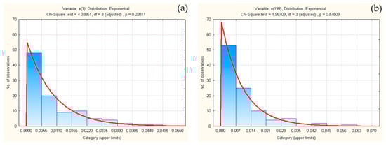
Figure 3. Verifications of exponential distributions for sets Δ↓[e(1)] (a) and Δ↓[e(199)] (b).

Figure 4 shows verifications of exponential distributions of all 200 sets of random numbers obtained from the successive decimals of constant e. All verifications were performed by χ² test, with a mandatory standard of 10 classes. The distribution of all 200 obtained significance thresholds is given in Figure 4. The distribution of all 200 obtained significance thresholds is given in Figure 4. From Figure 4 it is obvious that the verifications of the sets of random counts have periods of low verification. From Figure 4 it is obvious that the verifications of the sets of random counts have periods of low verification p < 0.05. These are the verifications (with the set index): p < 0.05. These are the verifications (with the set index): p₁₅₇ = 0.03111, p₁₅₈ = 0.00740, p₁₅₉ = 0.00740, p₁₆₀ = 0.00900, p₁₆₁ = 0.02863, p₁₆₂ = 0.01072, p₁₆₃ = 0.01072, p₁₆₄ = 0.01017, p₁₆₅ = 0.02065, p₁₆₉ = 0.03327, p₁₇₀ = 0.03327, p₁₇₂ = 0.03705, p₁₈₀ = 0.03282, p₁₈₁ = 0.02265, p₁₈₂ = 0.03890, p₁₈₃ = 0.04056, p₁₈₄ = 0.02192, p₁₈₅ = 0.03890, p₁₈₆ = 0.03890, p₁₈₇ = 0.03890, p₁₈₉ = 0.00865, p₁₉₁ = 0.03546 and p₁₉₂ = 0.02889. Out of a total of 200 sets of random numbers obtained on the basis of decimals of constant e, 23 sets have a significance threshold less than 0.05.

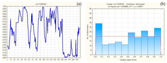
Figure 4. Exponential distributions of all 200 sets Δ↓[e(i)] (a), verifications, and distribution of verifications (b).

By the same procedure, consecutive differences were formed in 200 sets of random numbers obtained on the basis of successive decimals of a constant π(i), PRNG(i), and TRNG(i), i∈[1, 200].Figure 5 shows the results of 200 verifications of exponential distributions obtained from differences Δ↓[π(i)], i∈[1, 200] formed on the basis of successive decimals of a constant π(i), previously sorted ↓[π(i)].

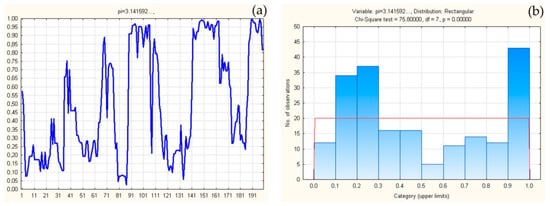
Figure 5. Exponential distributions of all 200 sets Δ↓[π(i)] (a), verifications, and distribution of verifications (b).

All verifications were performed by χ² test, according to the established standard of 10 classes. The distribution of all 200 obtained significance thresholds is given in Figure 5.

From Figure 5, it is obvious that the verifications of sets of random numbers are low verifications p < 0.05. These are the verifications (with the set index): p₈₃ = 0.00809 < 0.05, p₈₄ = 0.00809 < 0.05.

From a total of 200 sets of random numbers obtained based on the decimals of a constant π(i), i∈[1, 200], two sets have a significance threshold of less than 0.05.

Figure 6 shows the results of 200 verifications of exponential distributions obtained from differences Δ↓[PRNG(i)], i∈[1, 200], previously sorted ↓[PRNG(i)].

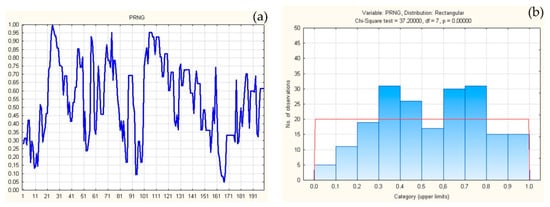
Figure 6. Exponential distributions of all 200 sets Δ↓[PRNG(i)] (a), verifications, and distribution of verifications (b).

All verifications were performed by χ² test, according to the established standard of 10 classes. The distribution of all 200 obtained significance thresholds is given in Figure 6.

From Figure 6 it is obvious that the verification of sets of random numbers has one low verification p < 0.05. This is the verification (with set index): p₁₆₇ = 0.04777 < 0.05. Out of a total of i∈[1, 200], one set has a significance threshold of less than 0.05.

Figure 7 shows the results of 200 verifications of exponential distributions obtained from differences Δ↓[TRNG(i)], i∈[1, 200], previously sorted ↓[TRNG(i)].

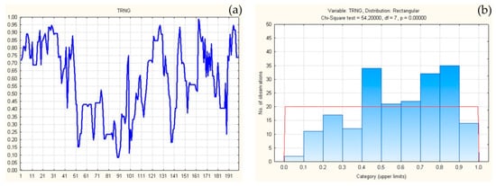
Figure 7. Exponential distributions of all 200 sets Δ↓[TRNG(i)] (a), verifications, and distribution of verifications (b).

All verifications were performed by χ² test, according to the established standard of 10 classes. The distribution of all 200 obtained significance thresholds is given in Figure 7.

All sets have a significant exponential distribution for the significance threshold p_i > 0.05, i∈[1, 200].

4. Discussion and Conclusions

The procedure for the application of exponential distribution in the testing of sets of random numbers is as follows: The series of n generated random numbers needs to be sorted by value. Next, succcessive differences are calculated for random numbers sorted by value. The random variable of successive differences needs to have a significant exponential distribution. If the exponential distribution with parameters E(n⁻¹, n⁻¹) is not verified, the set of generated random numbers are dependent and cannot be used.

Although it is the basis of many probabilistic functions, in this particular case it was proven that the constant e cannot be applied as a transcendental source of random numbers. With the fact that it is a sequence of e² purely-periodic with a period length of 40 [33], the sensitivity of the theorem is indirectly confirmed. For random numbers obtained from consecutive decimals of constant π, a significant departure from a uniform distribution [34] and randomness [35] was found. For random numbers generated from successive decimals of a constant e over 11.50% of sets are not exponentially distributed with a significance threshold p = 0.05, and for constant π this condition is not fulfilled in 1% of sets. According to results from the Diehard Battery of Tests (monkey tests, GCD, birthday spacing’s tests, parking lot test, squeeze test, etc.) the first 10⁹ digits of π and e all seem to pass the test very well [36].

It should be noted here that the mean of the significance threshold of all 200 verifications for the number e was E(p_e) = 0.526329 and was greater than the mean value of the significance threshold of all 200 verifications for the number π which was E(p_π) = 0.501486. The TRNG series did not meet the condition of exponential distribution in 0.5% (1 of 200), while the TRNG series fully met the condition of the theorem. The mean significance threshold of all 200 verifications for the PRNG series was E(p_PRNG) = 0.543097. Although higher E(p_e) and E(p_π), it was smaller than the mean significance threshold of 200 exponential distribution verification for TRNG sets-E(p_TRNG) = 0.589363. In total, the TRNG series had all significant verifications in all 200 sets of random numbers and had the highest mean of verifications.

The results of the first tests and the comparative results confirm the validity of the theorem. The idea based on the entropy of the exponential distribution and its memoryless properties is expressed in the mutual independence between the generated random numbers. The test is natural because a stochastic function with the highest entropy, an exponential distribution, is introduced into the quality testing of a set of random numbers.

Certainly, the standard test of the uniform distribution U[0,1] of generated random numbers is also a stochastic test. However, the test of the exponential distribution of consecutive differences between generated random numbers, absorbs the test of uniform distribution. In the case of the non-uniform distribution of generated random numbers, a large number of small and big consecutive differences will appear in the set of generated random numbers, which will prevent the verification of the exponential distribution with a significant threshold. In the case of repeating the same decimals while generating random numbers, a large number of small differences with the same non-verification outcome also occur, etc.

However, in the case of extremely large sets of generated random numbers, their consecutive differences converge to zero. According to the theorem and the parameters of the exponential distribution, the standard deviation of consecutive differences in large sets also converges to zero. This means that the proposed test has limitations, which need to be established. Despite this limitation, the proposed test can be applied for the primary selection of a series of generated random numbers. The estimated limit is based on the rare event standard [37] for the exponential distribution parameter λ = 10⁻⁶, or 1,000,000 consecutive random decimals.

References

- Gallager, R.G. Principles of Digital Communication, 1st ed.; Cambridge University Press: Cambridge, UK, 2008. [Google Scholar]
- Ferguson, N.; Schneier, B.; Kohno, T. Cryptography Engineering: Design Principles and Practical Applications, 1st ed.; John Wiley & Sons: New York, NY, USA, 2010. [Google Scholar]
- Wang, J.; Liang, J.; Li, P.; Yang, L.; Wang, Y. All-optical random number generating using highly nonlinear fibers by numerical simulation. Opt. Commun. 2014, 321, 1–5. [Google Scholar] [CrossRef]
- Joppich, G.; Däuper, J.; Dengler, R.; Johannes, S.; Rodriguez-Fornells, A.; Münte, T.F. Brain potentials index executive functions during random number generation. Neurosci. Res. 2004, 49, 57–164. [Google Scholar] [CrossRef] [PubMed]
- Bains, W. Random number generation and creativity. Med. Hypotheses 2008, 70, 186–190. [Google Scholar] [CrossRef] [PubMed]
- Brugger, P.; Monsch, A.U.; Salmon, D.P.; Butters, N. Random number generation in dementia of the Alzheimer type: A test of frontal executive functions. Neuropsychologia 1996, 34, 97–103. [Google Scholar] [CrossRef]
- Koike, S.; Takizawa, R.; Nishimura, Y.; Marumo, K.; Kinou, M.; Kawakubo, Y.; Rogers, M.A.; Kasai, K. Association between severe dorsolateral prefrontal dysfunction during random number generation random number generation and earlier onset in schizophrenia. Clin. Neurophysiol. 2011, 122, 1533–1540. [Google Scholar] [CrossRef]
- Anzak, A.; Gaynor, L.; Beigi, M.; Foltynie, T.; Limousin, P.; Zrinzo, L.; Brown, P.; Jahanshahi, M. Subthalamic nucleus gamma oscillations mediate a switch from automatic to controlled processing: A study of random number generation in Parkinson’s disease. NeuroImage 2013, 64, 284–289. [Google Scholar] [CrossRef] [PubMed]
- Linnebank, M.; Brugger, P. Random number generation deficits in patients with multiple sclerosis: Characteristics and neural correlates. Cortex 2016, 82, 237–243. [Google Scholar]
- Yadolah, D. A Natural Random Number Generator. Int. Stat. Rev. 1996, 64, 329–344. [Google Scholar]
- Yadolah, D.; Melfi, G. Random numbergenerators and rare events in the continued fraction of π. J. Stat. Comput. Simul. 2005, 75, 189–197. [Google Scholar]
- Kanter, I.; Aviad, Y.; Reidler, I.; Cohen, E.; Rosenbluh, M. An optical ultrafast random bit generator. Nat. Photonics 2010, 4, 58–61. [Google Scholar] [CrossRef]
- Lucian, L. FPGA optimized cellular automaton random number generator. J. Parallel Distrib. Comput. 2018, 111, 251–259. [Google Scholar]
- Panneton, F.; L’Ecuyer, P. Resolution-stationary random number generators. Math. Comput. Simul. 2010, 80, 1096–1103. [Google Scholar] [CrossRef]
- Fleischer, K. Two tests of pseudo random number generators for independence and uniform distribution. J. Stat. Comput. Simul. 1995, 52, 311–322. [Google Scholar] [CrossRef]
- Geisseler, O.; Pflugshaupt, T.; Buchmann, A.; Bezzola, L.; Reuter, K.; Schuknecht, B.; Weller, D.; L’Ecuyer, P. Tests based on sum-functions of spacings for uniform random numbers. J. Stat. Comput. Simul. 1997, 59, 251–269. [Google Scholar]
- Tomassini, M.; Sipper, M.; Zolla, M.; Perrenoud, M. Generating high-quality random numbers in parallel by cellular automata. Future Gener. Comput. Syst. 1999, 16, 291–305. [Google Scholar] [CrossRef]
- Díaz, N.C.; Gil, A.V.; Vargas, M.J. Assessment of the suitability of different random number generators for Monte Carlo simulations in gamma-ray spectrometry. Appl. Radiat. Isot. 2010, 68, 469–473. [Google Scholar] [CrossRef] [PubMed]
- Van Bever, G. Simplicial bivariate tests for randomness. Stat. Probab. Lett. 2016, 112, 20–25. [Google Scholar] [CrossRef]
- Knuth, D. The Art of Computer Programming: Seminumerical Algorithms, 3rd ed.; Addison-Wesley Longman Publishing Co., Inc.: Boston, MA, USA, 1997. [Google Scholar]
- Marsaglia, G.; Tsang, W. Some Difficult-to-pass Tests of Randomness. J. Stat. Softw. 2002, 7, 1–9. [Google Scholar] [CrossRef]
- McCullough, B.D. A Review of TestU01. J. Appl. Econ. 2006, 21, 677–682. [Google Scholar] [CrossRef]
- Rukhin, A.; Soto, J.; Nechvatal, J.; Smid, M.; Barker, E.; Leigh, S.; Levenson, M.; Vangel, M.; Banks, D.; Heckert, A.; et al. A Statistical Test Suite for Random and Pseudorandom Number Generators for Cryptographic Applications; National Institute of Standards and Technology; U.S. Department of Commerce: Washington, DC, USA, 2010.
- Steffensen, J.F. Some Recent Research in the Theory of Statistics and Actuarial Science; Cambridge University Press: Cambridge, UK, 1930. [Google Scholar]
- Kinzer, J.P. Application of The Theory of Probability to Problems of Highway Traffic, B.C.E. Doctoral Thesis, Polytechnic Institute of Brooklyn, New York, NY, USA, 1933. [Google Scholar]
- Teissier, F. Researches sur le vieillissement et sur les lios se mortalit. Ann. Phys. Biol. Phys. Chemestry 1934, 10, 237–264. [Google Scholar]
- Adams, W.F. Road Traffic Considered as a Random Series. J. Inst. Civ. Eng. 1936, 4, 121–130. [Google Scholar] [CrossRef]
- Weibull, W. The phenomenon of rupture in solids. Ingeniorsvetenskapsakademienshandlingar 1939, 153, 1–55. [Google Scholar]
- Kendall, M.G.; Smith, B.; Babington, B. Randomness and Random Sampling Numbers. J. R. Stat. Soc. 1938, 101, 147–166. [Google Scholar] [CrossRef]
- Kjos-Hanssen, B.; Taveneaux, A.; Thapen, N. How much randomness is needed for statistics? Ann. Pure Appl. Log. 2014, 165, 1470–1483. [Google Scholar] [CrossRef]
- Vukadinović, S. Queueing Systems; NaučnaKnjiga: Beograd, Serbia, 1988. [Google Scholar]
- Random Sequence Generator. Available online: https://www.random.org/sequences (accessed on 19 May 2019).
- Girstmair, K. Jacobi symbols and Euler′s number e. J. Number Theory 2014, 135, 155–166. [Google Scholar] [CrossRef]
- Khodabin, M. Some Wonderful Statistical Properties of Pi-number decimal digits. J. Math. Sci. Adv. Appl. 2011, 11, 69–77. [Google Scholar]
- Ganc, E.R. The Decimal Expansion of π Is Not Statistically Random. Exp. Math. 2014, 23, 99–104. [Google Scholar]
- Marsaglia, G. On the randomness of pi and other decimal expansions. InterStat: Statistics on the Internet, p. 17, October 2005. ISSN 1941-689X. Available online: http://interstat.statjournals.net/YEAR/2005/articles/ 0510005.pdf (accessed on 25 September 2019).
- Tanackov, I.; Jevtić, Ž.; Stojić, G.; Feta, S.; Ercegovac, P. Rare events queueing system. Oper. Res. Eng. Sci. Theory Appl. 2019, 2, 1–11. [Google Scholar] [CrossRef]
© 2019 by the authors. Licensee MDPI, Basel, Switzerland. This article is an open access article distributed under the terms and conditions of the Creative Commons Attribution (CC BY) license (http://creativecommons.org/licenses/by/4.0/).