Computation of Topological Indices of Some Special Graphs

Abstract

There are several chemical indices that have been introduced in theoretical chemistry to measure the properties of molecular topology, such as distance-based topological indices, degree-based topological indices and counting-related topological indices. Among the degree-based topological indices, the atom-bond connectivity ($ABC$) index and geometric–arithmetic ($GA$) index are the most important, because of their chemical significance. Certain physicochemical properties, such as the boiling point, stability and strain energy, of chemical compounds are correlated by these topological indices. In this paper, we study the molecular topological properties of some special graphs. The indices $(ABC)$, $(AB{C}_4)$, $(GA)$ and $(G{A}_5)$ of these special graphs are computed.

1. Introduction

Graph theory, as applied in the study of molecular structures, represents an interdisciplinary science called chemical graph theory or molecular topology. By using tools taken from graph theory, set theory and statistics, we attempt to identify structural features involved in structure–property activity relationships. Molecules and modeling unknown structures can be classified by the topological characterization of chemical structures with desired properties. Much research has been conducted in this area in the last few decades. The topological index is a numeric quantity associated with chemical constitutions purporting the correlation of chemical structures with many physicochemical properties, chemical reactivity or biological activity. Topological indices are designed on the grounds of the transformation of a molecular graph into a number that characterizes the topology of the molecular graph. We study the relationship between the structure, properties, and activity of chemical compounds in molecular modeling. Molecules and molecular compounds are often modeled by molecular graphs. A chemical graph is a model used to characterize a chemical compound. A molecular graph is a simple graph whose vertices correspond to the atoms and whose edges correspond to the bonds. It can be described in different ways, such as by a drawing, a polynomial, a sequence of numbers, a matrix or by a derived number called a topological index. The topological index is a numeric quantity associated with a graph, which characterizes the topology of the graph and is invariant under a graph automorphism. Some major types of topological indices of graphs are degree-based topological indices, distance-based topological indices and counting-related topological indices. The degree-based topological indices, the atom-bond connectivity ($ABC$) and geometric–arithmetic ($GA$) indices, are of great importance, with a significant role in chemical graph theory, particularly in chemistry. Precisely, a topological index $Top(G)$ of a graph is a number such that, if H is isomorphic to G, then $Top(H)$ = $Top(G)$. It is clear that the number of edges and vertices of a graph are topological indices [1,2,3,4,5,6,7]. We let $G=(V,E)$ be a simple graph, where $V(G)$ denotes its vertex set and $E(G)$ denotes its edge set. For any vertex $u\in V(G)$, we call the set $N_G(u)=\{v\in V(G)|uv\in E(G)\}$ the open neighborhood of u; we denote by $d_u$ the degree of vertex u and by $S_u={\sum }_{v\in N_G(u)}d(v)$ the degree sum of the neighbors of u. The number of vertices and number of edges of the graph G are denoted by $|V(G)|$ and $|E(G)|$, respectively. A simple graph of order n in which each pair of distinct vertices is adjacent is called a complete graph and is denoted by $K_n$. The notation in this paper is taken from the books [3,8,9,10].

In this paper, we study the molecular topological properties of some special graphs: Cayley trees, ${\Gamma }_n^2$; square lattices, $S{L}_n$; a graph $G_n$; and a complete bipartite graph, $K_{m,n}$. Additionally, the indices $(ABC)$, $(AB{C}_4)$, $(GA)$ and $(G{A}_5)$ of these special graphs, whose definitions are discussed in the materials and methods section, are computed.

Definition 1.

[11] The oldest degree-based topological index, the Randi’c index, denoted by $R_{-}\frac{1}{2}(G)$, is defined as

$$R_{-\frac{1}{2}}(G)=\sum _{uv\in E(G)}\frac{1}{\sqrt{d_u{d}_v}}.$$

(1)

Definition 2.

[12] For any real number $\alpha \in \mathbb{R}$, the general Randi’c index, $R_{\alpha }(G)$, is defined as

$$R_{\alpha }(G)=\sum _{uv\in E(G)}{(d_u{d}_v)}^{\alpha }.$$

(2)

Definition 3.

[13]. The degree-based topological ABC index is defined as

$$ABC(G)=\sum _{uv\in E(G)}\sqrt{\frac{d_u+d_v-2}{d_u{d}_v}}.$$

(3)

Definition 4.

[2]. The degree-based topological GA index is defined as

$$GA(G)=\sum _{uv\in E(G)}\frac{2\sqrt{d_u{d}_v}}{d_u+d_v}.$$

(4)

Recently, several authors have introduced new versions of the $ABC$ and $GA$ indices, which we derive in the two definitions below.

Definition 5.

[14]. The fourth version $(AB{C}_4)$ of the ABC index is defined as

$$AB{C}_4(G)=\sum _{uv\in E(G)}\sqrt{\frac{S_u+S_v-2}{S_u{S}_v}}.$$

(5)

Definition 6.

[15]. The fifth version $(G{A}_5)$ of the GA index is defined as

$$G{A}_5(G)=\sum _{uv\in E(G)}\frac{2\sqrt{S_u{S}_v}}{S_u+S_v}.$$

(6)

The concept of topological indices came from Wiener [16] while he was working on the boiling point of paraffin and was named the index path number. Later, the path number was renamed as the Wiener index [17]. Hayat et al. [1] studied various degree-based topological indices for certain types of networks, such as silicates, hexagonals, honeycombs and oxides. Imran et al. [7] studied the molecular topological properties and determined the analytical closed formula of the $ABC$, $AB{C}_4$ , $AB{C}_5$ , $GA$, $G{A}_4$ and $G{A}_5$ indices of Sierpinski networks. M. Darafsheh [18] developed different methods to calculate the Wiener index, Szeged index and Padmakar–Ivan index for various graphs using the group of automorphisms of G. He also found the Wiener indices of a few graphs using inductive methods. A. Ayache and A. Alameri [19] provided some topological indices of $m^k$-graphs, such as the Wiener index, the hyper-Wiener index, the Wiener polarity, Zagreb indices, Schultz and modified Schultz indices and the Wiener-type invariant. Wei Gao et al. [20] obtained certain eccentricity-version topological indices of the family of cycloalkanes $C_n^{R_i}$. Recently, there has been extensive research into $ABC$ and $GA$ indices, as well as into their variants. For further studies of topological indices of various graphs and chemical structures, see [21,22,23,24,25,26].

2. Materials and Methods

2.1. The Cayley Tree ${\Gamma }^k$

The Cayley tree ${\Gamma }^k$ of order $k\ge 1$ is an infinite and symmetric regular tree, that is, a graph without cycles, from each vertex of which exactly $k+1$ edges are issued. In this paper, we consider the Cayley tree ${\Gamma }_n^2=(V,E,i)$ of order 2 and with n levels from the root $x_0$, where V is the set of vertices of ${\Gamma }_n^2$, E is the set of edges of ${\Gamma }_n^2$, and i is the incidence function associating each edge $e\in E$ with its end vertices. If $i(e)=\{x,y\}$, then x and y are adjacent vertices, and we write $e=<x,y>$. For any $x,y\in V$, the distance $d(x,y)$ is defined as

$$d(x,y)=min\{d|x=x_0,x_1,x_2,\dots ,x_{d-1},x_d=y\in V\}$$

such that the pairs $<x_0,x_1>,<x_1,x_2>,\dots ,<x_{d-1},x_d>$ are adjacent vertices [27].

For the root $x_0$ of the Cayley tree, we have

$$W_n=\{x\in V|d(x_0,x)=n\},$$

$$V_n=\{x\in V|d(x_0,x)\le n\},$$

$$E_n=\{e=<x,y>\in E|x,y\in V_n\}.$$

It is easy to compute the number of vertices reachable in step n or in level n starting from the root $x_0$, which is $|W_n|=3\times 2^{(n-1)}$. The number of vertices of ${\Gamma }_n^2$ is $|V_n|=1+3\times (2^n-1)$, and the number of edges of ${\Gamma }_n^2$ is $|E_n|=3\times (2^n-1)$, as is shown in Figure 1 below.

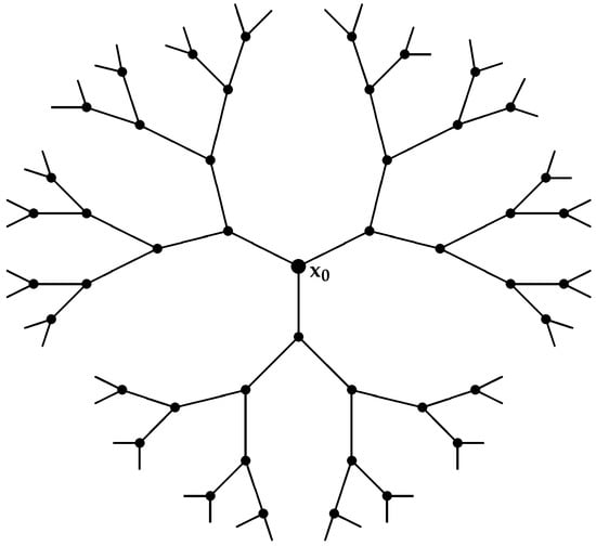
Figure 1. Cayley tree ${\Gamma }_n^2$ of order 2 with n levels, where $n\ge 1$.

2.2. The Square Lattice Graph $S{L}_n$

Lattice networks are widely used, for example, in distributed parallel computation, distributed control, wired circuits, and so forth. They are also known as grid or mesh networks. We choose a simple structure of lattice networks called a square lattice because this allows for a theoretical analysis [28].

We consider a square graph $S{L}_n(V,E)$ of size $n\times n$ vertices, where V denotes the set of vertices of $S{L}_n$ and E denotes the set of edges of $S{L}_n$, such that the number of vertices is $|V|=n^2$, and the number of edges is $|E|=2n(n-1)$, as is shown in Figure 2 below.

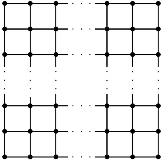
Figure 2. Square lattice ($S{L}_n$) with $n\ge 1$.

2.3. The Special Graph $G_n$

Other kinds of special graphs, denoted by $G_n$, can be obtained from other subgraphs. The structures in Figure 3 show how to obtain a graph $G_n$.

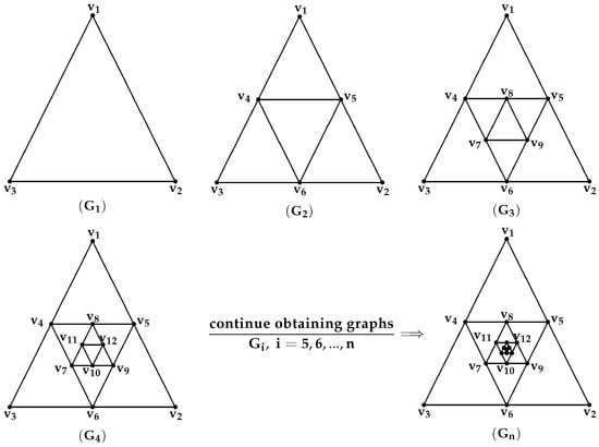
Figure 3. Structures of graphs ${\mathbf{G}}_{\mathbf{1}}$, ${\mathbf{G}}_{\mathbf{2}}$, ${\mathbf{G}}_{\mathbf{3}}$, ${\mathbf{G}}_{\mathbf{4}}$ …, ${\mathbf{G}}_{\mathbf{n}}$ of orders 3, 6, 9, 12, …, 3n.

In Figure 3, we have obtained the graph sequence $G_1,G_2,G_3,G_4,\dots ,G_n$. We let $G_1$ be a complete graph of order 3 ($G_1\equiv K_3$) and let $V(G_1)=\{v_1,v_2,v_3\}$; we have subdivided the three edges of $G_1$. The new vertices are denoted by $\{v_4,v_5,v_6\}$, and $G_2[v_4,v_5,v_6]\equiv K_3$. Thus,

• $V(G_2)=V(G_1)\cup \{v_1,v_2,v_3\},$
• $E(G_2)=\{v_1{v}_5,v_5{v}_2,v_2{v}_6,v_6{v}_3,v_3{v}_4,v_4{v}_1,v_4{v}_5,v_5{v}_6,v_6{v}_4\},$
• $G_2=G_1-\{v_1{v}_2,v_2{v}_3,v_3{v}_1\}+\{v_1{v}_5,v_5{v}_2,v_2{v}_6,v_6{v}_3,v_3{v}_4,v_4{v}_1,v_4{v}_5,v_5{v}_6,v_6{v}_4\}.$

Now, for $G_n$, we have subdivided the edges $\{v_{3n-5}{v}_{3n-4},v_{3n-4}{v}_{3n-3},v_{3n-3}{v}_{3n-5}\}$. The new vertices are denoted by $\{v_{3n-2},v_{3n-1},v_{3n}\}$ and $G_n[v_{3n-2},v_{3n-1},v_{3n}]\equiv K_3$. Thus,

• $V(G_n)=V(G_{n-1})\cup \{v_{3n-2},v_{3n-1},v_{3n}\}$,
• $G_n=G_{n-1}-\{v_{3n-5}{v}_{3n-4},v_{3n-4}{v}_{3n-3},v_{3n-3}{v}_{3n-5}\}+\{v_{3n-5}{v}_{3n},v_{3n}{v}_{3n-4},v_{3n-4}{v}_{3n-2},v_{3n-2}{v}_{3n-3},v_{3n-3}{v}_{3n-1},v_{3n-1}{v}_{3n-5},v_{3n-2}{v}_{3n-1},v_{3n-1}{v}_{3n},v_{3n}{v}_{3n-2}\}.$

It can be observed that the number of vertices of a graph $G_n$ is $3n$ and that the number of edges is $6n-3$ or, mathematically, $|V(G_n)|=3n$, and $|E(G_n)|=6n-3$, respectively, where $n\ge 1$.

2.4. The Complete Bipartite Graph $K_{m,n}$

A graph $K_{m,n}$ is a complete bipartite graph if its vertex set can be partitioned into two subsets X and Y, such that one of the two endpoints of each edge in X and the other in Y, as well as each vertex $v\in X$, is adjacent to all vertices of Y, as is shown in Figure 4 below. Clearly, if $|X|=m$ and $|Y|=n$, then $|V(K_{m,n})|=m+n$ and $|E(K_{m,n})|=mn$. For more details, see [10].

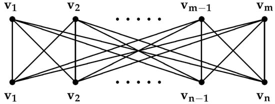
Figure 4. Complete bipartite graph $K_{m,n}$.

3. Results and Discussion

Prior to presenting our main results, the edge partitions of the Cayley tree, lattice square, $G_n$ and complete bipartite graph, on the basis of the degrees of end vertices of each edge and the degree sum of the neighbors of end vertices of each edge, are discussed below.

Referring to Figure 1, there are two types of edges in ${\Gamma }_n^2$ on the basis of the degrees of the end vertices of each edge, as follows: the first type, for $e=uv\in E({\Gamma }_n^2)$, is such that $d_u=1$ and $d_v=3$; the other type is, for $e=uv\in E({\Gamma }_n^2)$ such $d_u=d_v=3.$ In the first type, there are $3\times 2^{n-1}$ edges, and in the other type, because $|E({\Gamma }_n^2)|=3\times (2^n-1)$, there are $3\times (2^n-1)-3\times 2^{n-1}=3\times (2^n-2^{n-1}-1)=3\times (2^{n-1}-1)$ edges, as is shown in Table 1. Similarly, from Figure 1, there are three types of edges in ${\Gamma }_n^2$ on the basis of the degree sum of vertices lying at a unit distance from the end vertices of each edge, as follows: the first type, for $e=uv\in E({\Gamma }_n^2)$, is such that $S_u=3$ and $S_v=5$; the second type, for $e=uv\in E({\Gamma }_n^2)$, is such that $S_u=5$ and $S_v=9$; the third type, for $e=uv\in E({\Gamma }_n^2)$, is such that $S_u=S_v=9.$ There are $3\times 2^{n-1}$, $3\times 2^{n-2}$, and $3\times (2^n-1)-3\times 2^{n-1}-3\times 2^{n-2}=3(2^n-2^{n-1}-2^{n-2}-1)=3\times 2^{n-2}$ edges in the first, second and third types of ${\Gamma }_n^2$, respectively, as is shown in Table 2.

Table 1. Edge partition of ${\Gamma }_n^2$ on the basis of degrees of end vertices of each edge.

(${\mathit{d}}_{\mathit{u}}\mathbf{,}{\mathit{d}}_{\mathit{v}}$) Where $\mathit{u}\mathit{v}\mathbf{\in }\mathit{E}$	Number of Edges
(1, 3)	$3\times 2^{n-1}$
(3, 3)	$3\times (2^{(n-1)}-1)$

Table 2. Edge partition of ${\Gamma }_n^2$ on the basis of degree sum of neighbors of end vertices of each edge.

(${\mathit{S}}_{\mathit{u}}\mathbf{,}{\mathit{S}}_{\mathit{v}}$) Where $\mathit{u}\mathit{v}\mathbf{\in }\mathit{E}$	Number of Edges
(3, 5)	$3\times 2^{n-1}$
(5, 9)	$3\times 2^{n-2}$
(9, 9)	$3\times (2^{(n-2)}-1)$

Referring to Figure 2, there are four types of edges in $S{L}_n$ on the basis of the degrees of the end vertices of each edge, as follows: the first type, for $e=uv\in E(S{L}_n)$, is such that $d_u=2$ and $d_v=3$; the second type, for $e=uv\in E(S{L}_n)$, is such that $d_u=3$ and $d_v=3$; the third type, for $e=uv\in E(S{L}_n)$, is such that $d_u=3$ and $d_v=4$; the fourth type, for $e=uv\in E(S{L}_n)$, is such that $d_u=d_v=4$. Because $|E(S{L}_n)|=2n(n-1)$, then there are 8, $4(n-3)$, $4(n-2)$, and $2n(n-1)-[8+4(n-3)+4(n-2)]=2n^2-2n-[8+4n-12+4n-8]=2n^2-10n-12$ edges in the first, second, third and fourth types of $S{L}_n$, respectively, as is shown in Table 3.

Table 3. Edge partition of $S{L}_n$ on the basis of degrees of end vertices of each edge.

(${\mathit{d}}_{\mathit{u}}\mathbf{,}{\mathit{d}}_{\mathit{v}}$) Where $\mathit{u}\mathit{v}\mathbf{\in }\mathit{E}$	Number of Edges
(2, 3)	8
(3, 3)	$4(n-3)$
(3, 4)	$4(n-2)$
(4, 4)	$2n^2-10n+12$

Similarly, from Figure 2, there are nine types of edges in $S{L}_n$ on the basis of the degree sum of vertices lying at a unit distance from the end vertices of each edge, as follows:

• For $e=uv\in E(S{L}_n)$ such that $S_u=6$ and $S_v=9$, there are 8 edges.
• For $e=uv\in E(S{L}_n)$ such that $S_u=9$ and $S_v=10$, there are 8 edges.
• For $e=uv\in E(S{L}_n)$ such that $S_u=10$ and $S_v=10$, there are $4(n-5)$ edges.
• For $e=uv\in E(S{L}_n)$ such that $S_u=9$ and $S_v=14$, there are 8 edges.
• For $e=uv\in E(S{L}_n)$ such that $S_u=10$ and $S_v=15$, there are $4(n-4)$ edges.
• For $e=uv\in E(S{L}_n)$ such that $S_u=14$ and $S_v=15$, there are 8 edges.
• For $e=uv\in E(S{L}_n)$ such that $S_u=15$ and $S_v=15$, there are $4(n-5)$ edges.
• For $e=uv\in E(S{L}_n)$ such that $S_u=15$ and $S_v=16$, there are $4(n-4)$ edges.
• For $e=uv\in E(S{L}_n)$ such that $S_u=16$ and $S_v=16$, and because $|E(S{L}_n)|=2n(n-1)$, then there are $2n(n-1)-[32+8(n-5)+8(n-4)]=2n^2-2n-[16n-40]=2n^2-18n+40$ edges.

Table 4 shows the edge partition of the square lattice $S{L}_n$ on the basis of the degree sum of vertices lying at a unit distance from the end vertices of each edge.

Table 4. Edge partition of $S{L}_n$ on the basis of degree sum of neighbors of end vertices of each edge.

(${\mathit{S}}_{\mathit{u}}\mathbf{,}{\mathit{S}}_{\mathit{v}}$) Where $\mathit{u}\mathit{v}\mathbf{\in }\mathit{E}$	Number of Edges
(6, 9)	8
(9, 10)	8
(10, 10)	$4(n-5)$
(9, 14)	8
(10, 15)	$4(n-4)$
(14, 15)	8
(15, 15)	$4(n-5)$
(15, 16)	$4(n-4)$
(16, 16)	$2n^2-18n+40$

Referring to Figure 3, for the edge partition of $G_n$ on the basis of the degrees of the end vertices of each edge, we have two cases for $n=1$ and $n\ge 2$, as follows:

For $n=1$, because $G_1\equiv K_3$, then there are 3 edges such that $d_u=d_v=2$, as is shown in Table 5.

Table 5. Edge partition of $G_n$ $(n=1)$ on the basis of degrees of end vertices of each edge.

(${\mathit{d}}_{\mathit{u}}\mathbf{,}{\mathit{d}}_{\mathit{v}}$) Where $\mathit{u}\mathit{v}\mathbf{\in }\mathit{E}$	Number of Edges
(2, 2)	3

For $n\ge 2$, there are two types of edges in $G_n$, as follows: the first type, for $e=uv\in E(G_n)$, is such that $d_u=2$ and $d_v=4$; the other type, for $e=uv\in E(G_n)$, is such that $d_u=d_v=4$. In the first type, there are 6 edges, and in the other type, because $|E(G_n)|=6n-3$, then there are $(6n-3)-6=6n-9$ edges, as is shown in Table 6.

Table 6. Edge partition of $G_n$ $(n\ge 2)$ on the basis of degrees of end vertices of each edge.

(${\mathit{d}}_{\mathit{u}}\mathbf{,}{\mathit{d}}_{\mathit{v}}$) Where $\mathit{u}\mathit{v}\mathbf{\in }\mathit{E}$	Number of Edges
(2, 4)	6
(4, 4)	$6n-9$

Similarly, from Figure 3, for the edge partition of $G_n$ on the basis of the degree sum of vertices lying at a unit distance from the end vertices of each edge, we have three cases for $n=1$, $n=2$ and $n\ge 3$, as follows:

For $n=1$, because $G_1\equiv K_3$, then there are 3 edges such that $S_u=S_v=4$, as is shown in Table 7.

Table 7. Edge partition of $G_n$ $(n=1)$ on the basis of degree sum of neighbors of end vertices of each edge.

(${\mathit{S}}_{\mathit{u}}\mathbf{,}{\mathit{S}}_{\mathit{v}}$) Where $\mathit{u}\mathit{v}\mathbf{\in }\mathit{E}$	Number of Edges
(4, 4)	3

For $n=2$, there are two types of edges in $G_2$, as follows: the first type, for $e=uv\in E(G_2)$, is such that $S_u=8$ and $S_v=12$; the other type, for $e=uv\in E(G_2)$, is such that $S_u=S_v=12$. There are 6 edges in the first type of $G_2$ and 3 edges in the second type of $G_2$, as is shown in Table 8.

Table 8. Edge partition of $G_n$ $(n=2)$ on the basis of degree sum of neighbors of end vertices of each edge.

(${\mathit{S}}_{\mathit{u}}\mathbf{,}{\mathit{S}}_{\mathit{v}}$) Where $\mathit{u}\mathit{v}\mathbf{\in }\mathit{E}$	Number of Edges
(8, 12)	6
(12, 12)	3

For $n\ge 3$, there are three types of edges in $G_n$, as follows: the first type, for $e=uv\in E(G_n)$, is such that $S_u=8$ and $S_v=12$; the second type, for $e=uv\in E(G_n)$, is such that $S_u=12$ and $S_v=16$; the third type, for $e=uv\in E(G_n)$, is such that $S_u=S_v=16$. There are 6 $edges$ in both the first type and the second type of $G_n$, and because $|E(G_n)|=6n-3$, then there are $(6n-3)-6-6=6n-15$ edges, as is shown in Table 9.

Table 9. Edge partition of $G_n$ $(n\ge 3)$ on the basis of degree sum of neighbors of end vertices of each edge.

(${\mathit{S}}_{\mathit{u}}\mathbf{,}{\mathit{S}}_{\mathit{v}}$) Where $\mathit{u}\mathit{v}\mathbf{\in }\mathit{E}$	Number of Edges
(8, 12)	6
(12, 16)	6
(16, 16)	$6n-15$

Referring to Figure 4, for the complete bipartite graph $K_{m,n}$, because $\forall u\in X,d_u=m$ and $\forall v\in Y,d_v=n$, where $|E(K_{m,n})|=mn$, then the number of edges of $K_{m,n}$ on the basis of the degrees of the end vertices of each edge is such that $d_u=m$, and $d_v=n$ is equal to the number of edges of $K_{m,n}$ on the basis of the degree sum of the vertices lying at a unit distance from the end vertices of each edge such that $S_u=S_v=mn$ and both of them are equal to $mn$, as is shown in Table 10 and Table 11 respectively.

Table 10. Edge partition of $K_{m,n}$ on the basis of degrees of end vertices of each edge.

(${\mathit{d}}_{\mathit{u}}\mathbf{,}{\mathit{d}}_{\mathit{v}}$) Where $\mathit{u}\mathit{v}\mathbf{\in }\mathit{E}$	Number of Edges
($m,n$)	$mn$

Table 11. Edge partition of $K_{m,n}$ on the basis of degree sum of neighbors of end vertices of each edge.

(${\mathit{S}}_{\mathit{u}}\mathbf{,}{\mathit{S}}_{\mathit{v}}$) Where $\mathit{u}\mathit{v}\mathbf{\in }\mathit{E}$	Number of Edges
($mn$, $mn$)	$mn$

Using the data of the edge partition, which is presented in Table 1, Table 2, Table 3, Table 4, Table 5, Table 6, Table 7, Table 8, Table 9, Table 10 and Table 11, we can derive the following theorems.

Theorem 1.

For the Cayley tree ${\Gamma }_n^2$, the ABC index and the fourth version $(AB{C}_4)$ of the ABC index are equal to the following, respectively:

1. 

$ABC({\Gamma }_n^2)=2^{n-1}(3\sqrt{\frac{2}{3}}+2)-2$.

2. 

$AB{C}_4({\Gamma }_n^2)=3\times 2^{n-1}\left(\sqrt{\frac{6}{15}}+\frac{1}{\sqrt{15}}+\frac{2}{9}\right)-\frac{4}{3}$.

Proof 

• From Table 1, by using the edge partition of ${\Gamma }_n^2$ on the basis of the degrees of the end vertices of each edge, and because

  $$ABC(G)=\sum _{uv\in E(G)}\sqrt{\frac{d_u+d_v-2}{d_u{d}_v}},$$

  this implies that
  $ABC({\Gamma }_n^2)=3\times 2^{n-1}\sqrt{\frac{1+3-2}{1\times 3}}+3\times (2^{n-1}-1)\sqrt{\frac{3+3-2}{3\times 3}}.$
  After an easy simplification, we obtain
  $ABC({\Gamma }_n^2)=2^{n-1}(3\sqrt{\frac{2}{3}}+2)-2.$
• By using the edge partition of ${\Gamma }_n^2$ on the basis of the degree sum of the neighbors of the end vertices of each edge in Table 2, and because

  $$AB{C}_4(G)=\sum _{uv\in E(G)}\sqrt{\frac{S_u+S_v-2}{S_u{S}_v}},$$

  this implies that
  $AB{C}_4({\Gamma }_n^2)=3\times 2^{n-1}\sqrt{\frac{3+5-2}{3\times 5}}+3\times 2^{n-2}\sqrt{\frac{5+9-2}{5\times 9}}+3\times (2^{n-2}-1)\sqrt{\frac{9+9-2}{9\times 9}}.$
  After an easy simplification, we obtain
  $AB{C}_4({\Gamma }_n^2)=3\times 2^{n-1}\left(\sqrt{\frac{6}{15}}+\frac{1}{\sqrt{15}}+\frac{2}{9}\right)-\frac{4}{3}.$

By Equations (1) and (2), we complete the proof of the result. ☐

Theorem 2.

For the Cayley tree ${\Gamma }_n^2$, the GA index and the fifth version $(G{A}_5)$ of the GA index are equal to the following, respectively:

1. 

$GA({\Gamma }_n^2)=3\times 2^{n-2}(\sqrt{3}+2)-3.$

2. 

$G{A}_5({\Gamma }_n^2)=3\times 2^{n-3}(\sqrt{15}+\frac{6\sqrt{5}}{7}+2)-3.$

Proof 

• From Table 1 by using the edge partition of ${\Gamma }_n^2$ on the basis of the degrees of the end vertices of each edge, and because

  $$GA(G)=\sum _{uv\in E(G)}\frac{2\sqrt{d_u{d}_v}}{d_u+d_v},$$
  this gives that
  $GA({\Gamma }_n^2)=\frac{2\times 3\times 2^{n-1}\sqrt{1\times 3}}{1+3}+\frac{2\times 3\times (2^{n-1}-1)\sqrt{3\times 3}}{3+3}.$
  After an easy simplification, we obtain
  $GA({\Gamma }_n^2)=3\times 2^{n-2}(\sqrt{3}+2)-3.$
• By using the edge partition of ${\Gamma }_n^2$ on the basis of the degree sum of the neighbors of the end vertices of each edge shown in Table 2, and because

  $$G{A}_5(G)=\sum _{uv\in E(G)}\frac{2\sqrt{S_u{S}_v}}{S_u+S_v},$$
  this gives that
  $G{A}_5({\Gamma }_n^2)=\frac{2\times 3\times 2^{n-1}\sqrt{3\times 5}}{3+5}+\frac{2\times 3\times 2^{n-2}\sqrt{5\times 9}}{5+9}+\frac{2\times 3\times (2^{n-2}-1)\sqrt{9\times 9}}{9+9}.$
  After an easy simplification, we obtain
  $G{A}_5({\Gamma }_n^2)=3\times 2^{n-3}(\sqrt{15}+\frac{6\sqrt{5}}{7}+2)-3.$

By Equations (1) and (2), we complete the proof of the result. ☐

Theorem 3.

For the square lattice graph $S{L}_n$ the ABC index and the fourth version $(AB{C}_4)$ of the ABC index are equal to the following, respectively:

1. 

$ABC(S{L}_n)=\frac{8}{\sqrt{2}}+(n-3)\frac{8}{3}+2(n-2)\sqrt{\frac{5}{3}}+(n^2-10n+12)\frac{\sqrt{6}}{4}.$

2. 

$\begin{array}{cc}\hfill AB{C}_4(S{L}_n)& =\frac{8}{3}\sqrt{\frac{13}{6}}+\frac{8}{3}\sqrt{\frac{17}{10}}+\frac{6\sqrt{2}}{5}(n-5)+\frac{8}{3}\sqrt{\frac{3}{2}}+4\sqrt{\frac{23}{150}}(n-4)+\frac{24}{\sqrt{70}}+\frac{8\sqrt{7}}{15}(n-5)\hfill \\ & +\sqrt{\frac{29}{15}}(n-4)+\frac{\sqrt{30}}{16}(2n^2-18n+40).\hfill \end{array}$

Proof 

• From Table 3, by using the edge partition of $S{L}_n$ on the basis of the degrees of the end vertices of each edge, and because

  $$ABC(G)=\sum _{uv\in E(G)}\sqrt{\frac{d_u+d_v-2}{d_u{d}_v}},$$

  this implies that
  $ABC(S{L}_n)=8\sqrt{\frac{2+3-2}{2\times 3}}+4(n-3)\sqrt{\frac{3+3-2}{3\times 3}}+4(n-2)\sqrt{\frac{3+4-2}{3\times 4}}+(n^2-10n+12)\sqrt{\frac{4+4-2}{4\times 4}}.$
  After an easy simplification, we obtain
  $ABC(S{L}_n)=\frac{8}{\sqrt{2}}+(n-3)\frac{8}{3}+2(n-2)\sqrt{\frac{5}{3}}+(n^2-10n+12)\frac{\sqrt{6}}{4}.$
• By using the edge partition of $S{L}_n$ on the basis of the degree sum of the neighbors of the end vertices of each edge shown in Table 4, and because

  $$AB{C}_4(G)=\sum _{uv\in E(G)}\sqrt{\frac{S_u+S_v-2}{S_u{S}_v}},$$

  this implies that
  $\begin{array}{cc}\hfill AB{C}_4(S{L}_n)& =8\sqrt{\frac{6+9-2}{6\times 9}}+8\sqrt{\frac{9+10-2}{9\times 10}}+4(n-5)\sqrt{\frac{10+10-2}{10\times 10}}+8\sqrt{\frac{9+14-2}{9\times 14}}+4(n-4)\sqrt{\frac{10+15-2}{10\times 15}}\hfill \\ & +8\sqrt{\frac{14+15-2}{14\times 15}}+4(n-5)\sqrt{\frac{15+15-2}{15\times 15}}+4(n-4)\sqrt{\frac{15+16-2}{15\times 16}}+(2n^2-18n+40)\sqrt{\frac{16+16-2}{16\times 16}}.\hfill \end{array}$
  After an easy simplification, we obtain
  $\begin{array}{cc}\hfill AB{C}_4(S{L}_n)& =\frac{8}{3}\sqrt{\frac{13}{6}}+\frac{8}{3}\sqrt{\frac{17}{10}}+\frac{6\sqrt{2}}{5}(n-5)+\frac{8}{3}\sqrt{\frac{3}{2}}+4\sqrt{\frac{23}{150}}(n-4)+\frac{24}{\sqrt{70}}+\frac{8\sqrt{7}}{15}(n-5)\hfill \\ & +\sqrt{\frac{29}{15}}(n-4)+\frac{\sqrt{30}}{16}(2n^2-18n+40).\hfill \end{array}$

By Equations (1) and (2), we complete the proof of the result. ☐

Theorem 4.

For the square lattice graph $S{L}_n$ the GA index and the fifth version $(G{A}_5)$ of the GA index are equal to the following, respectively:

1. 

$GA(S{L}_n)=\frac{16\sqrt{6}}{5}+\frac{16\sqrt{3}}{7}(n-2)+(n^2-6n).$

2. 

$G{A}_5(S{L}_n)=\frac{16\sqrt{6}}{5}+\frac{48\sqrt{10}}{29}+\frac{48\sqrt{14}}{23}+\frac{8\sqrt{150}}{25}(n-4)+\frac{16\sqrt{210}}{29}+\frac{32\sqrt{15}}{31}(n-4)+(n^2-10n).$

Proof 

• From Table 3, by using the edge partition of $S{L}_n$ on the basis of the degrees of the end vertices of each edge, and because

  $$GA(G)=\sum _{uv\in E(G)}\frac{2\sqrt{d_u{d}_v}}{d_u+d_v},$$
  this gives that
  $GA(S{L}_n)=\frac{2\times 8\sqrt{2\times 3}}{2+3}+\frac{2\times 4(n-3)\sqrt{3\times 3}}{3+3}+\frac{2\times 4(n-2)\sqrt{3\times 4}}{3+4}+\frac{2\times (n^2-10n+12)\sqrt{4\times 4}}{4+4}.$
  After an easy simplification, we obtain
  $GA(S{L}_n)=\frac{16\sqrt{6}}{5}+\frac{16\sqrt{3}}{7}(n-2)+(n^2-6n).$
• By using the edge partition of $S{L}_n$ on the basis of the degree sum of the neighbors of the end vertices of each edge shown in Table 4, and because

  $$G{A}_5(G)=\sum _{uv\in E(G)}\frac{2\sqrt{S_u{S}_v}}{S_u+S_v},$$
  this gives that
  $G{A}_5(S{L}_n)=\frac{2\times 8\sqrt{6\times 9}}{6+9}+\frac{2\times 8\sqrt{9\times 10}}{9+10}+\frac{2\times 4(n-5)\sqrt{10\times 10}}{10+10}+\frac{2\times 8\sqrt{9\times 14}}{9+14}+\frac{2\times 4(n-4)\sqrt{10\times 15}}{10+15}+\frac{2\times 8\sqrt{14\times 15}}{14+15}+\frac{2\times 4(n-5)\sqrt{15\times 15}}{15+15}+\frac{2\times 4(n-4)\sqrt{15\times 16}}{15+16}+\frac{2\times (n^2-18n+40)\sqrt{16\times 16}}{16+16}.$
  After an easy simplification, we obtain
  $G{A}_5(S{L}_n)=\frac{16\sqrt{6}}{5}+\frac{48\sqrt{10}}{29}+\frac{48\sqrt{14}}{23}+\frac{8\sqrt{150}}{25}(n-4)+\frac{16\sqrt{210}}{29}+\frac{32\sqrt{15}}{31}(n-4)+(n^2-10n).$

By Equations (1) and (2), we complete the proof of the result. ☐

Theorem 5.

For the graph $G_n$, where $n=1$ and $n\ge 2$,the ABC index is equal to the following:

$$ABC(G_n)=\left\{\begin{array}{ccc}\frac{3}{2}\sqrt{2}\hfill & if\hfill & n=1,\hfill \\ 3\sqrt{2}+(6n-9)\frac{\sqrt{6}}{4}\hfill & if\hfill & n\ge 2.\hfill \end{array}\right.$$

Proof 

We prove this by using Table 5 and Table 6. We use the edge partition of $G_n$ on the basis of the degrees of the end vertices of each edge. Table 5 and Table 6 explain such a partition for the graph $G_n$ for $n=1$ and $n\ge 2$, respectively. Now by using the partitions given in Table 5 and Table 6, we can apply the formula of the $ABC$ index to compute this index for the graph $G_n$.

Because we have

$$ABC(G)=\sum _{uv\in E(G)}\sqrt{\frac{d_u+d_v-2}{d_u{d}_v}},$$

this gives, for $n=1$, $ABC(G_1)=3\sqrt{\frac{2+2-2}{2\times 2}}=3\sqrt{\frac{2}{4}}=\frac{3}{2}\sqrt{2}.$

For $n\ge 2$, because we have,

$$ABC(G)={\sum }_{uv\in E(G)}\sqrt{\frac{d_u+d_v-2}{d_u{d}_v}},$$

this gives $ABC(G_n)=6\sqrt{\frac{2+4-2}{2\times 4}}+(6n-9)\sqrt{\frac{4+4-2}{4\times 4}}=3\sqrt{2}+(6n-9)\frac{\sqrt{6}}{4}.$

This proves the result. ☐

Theorem 6.

For the graph $G_n$, where $n=1$ and $n\ge 2$, the GA index is equal to the following:

$$GA(G_n)=\left\{\begin{array}{ccc}3\hfill & if\hfill & n=1,\hfill \\ 4\sqrt{2}+(6n-9)\hfill & if\hfill & n\ge 2.\hfill \end{array}\right.$$

Proof 

We prove this by using Table 5 and Table 6. We use the edge partition of $G_n$ on the basis of the degrees of the end vertices of each edge. Table 5 and Table 6 explain such a partition for the graph $G_n$ for $n=1$ and $n\ge 2$, respectively. Now by using the partitions given in Table 5 and Table 6, we can apply the formula of the $GA$ index to compute this index for the graph $G_n$.

Because we have

$$GA(G)=\sum _{uv\in E(G)}\frac{2\sqrt{d_u{d}_v}}{d_u+d_v},$$

this implies, for $n=1$, $GA(G_1)=\frac{2\times 3\sqrt{2\times 2}}{2+2}=\frac{2\times 3\sqrt{4}}{4}=3.$

For $n\ge 2$, because we have

$$GA(G)={\sum }_{uv\in E(G)}\frac{2\sqrt{d_u{d}_v}}{d_u+d_v},$$

this implies that $GA(G_n)=\frac{2\times 6\sqrt{2\times 4}}{2+4}+\frac{2\times (6n-9)\sqrt{4\times 4}}{4+4}=4\sqrt{2}+(6n-9).$

This proves the result.  ☐

Theorem 7.

For the graph $G_n$, where $n=1, n=2$ and $n\ge 3$, the fourth version $(AB{C}_4)$ of the ABC index is equal to the following:

$$AB{C}_4(G_n)=\left\{\begin{array}{ccc}\frac{3}{4}\sqrt{6}\hfill & if\hfill & n=1,\hfill \\ \frac{3\sqrt{3}}{2}+\frac{\sqrt{22}}{4}\hfill & if\hfill & n=2,\hfill \\ \frac{3\sqrt{3}}{2}+\frac{3}{2}\sqrt{\frac{13}{6}}+(6n-15)\frac{\sqrt{30}}{16}\hfill & if\hfill & n\ge 3.\hfill \end{array}\right.$$

Proof 

We prove this by using Table 7, Table 8 and Table 9. We use the edge partition of $G_n$ on the basis of the degree sum of the neighbors of the end vertices of each edge. Table 7, Table 8 and Table 9 explain such a partition for the graph $G_n$ for $n=1$, $n=2$ and $n\ge 3$, respectively. Now by using the partitions given in Table 7, Table 8 and Table 9, we can apply the formula of the $AB{C}_4$ index to compute this index for the graph $G_n$.

Because we have

$$AB{C}_4(G)=\sum _{uv\in E(G)}\sqrt{\frac{S_u+S_v-2}{S_u{S}_v}},$$

this gives, for $n=1$, $AB{C}_4(G_1)=3\sqrt{\frac{4+4-2}{4\times 4}}=\frac{3}{4}\sqrt{6}.$

For $n=2$, because we have

$$AB{C}_4(G)={\sum }_{uv\in E(G)}\sqrt{\frac{S_u+S_v-2}{S_u{S}_v}},$$

this gives $AB{C}_4(G_2)=6\sqrt{\frac{8+12-2}{8\times 12}}+3\sqrt{\frac{12+12-2}{12\times 12}}.$

After an easy simplification, we obtain

$$AB{C}_4(G_2)=\frac{3\sqrt{3}}{2}+\frac{\sqrt{22}}{4}.$$

For $n\ge 3,$ because we have,

$$AB{C}_4(G)={\sum }_{uv\in E(G)}\sqrt{\frac{S_u+S_v-2}{S_u{S}_v}},$$

this gives $AB{C}_4(G_n)=6\sqrt{\frac{8+12-2}{8\times 12}}+6\sqrt{\frac{12+16-2}{12\times 16}}+(6n-15)\sqrt{\frac{16+16-2}{16\times 16}}.$

After an easy simplification, we obtain

$$AB{C}_4(G_n)=\frac{3\sqrt{3}}{2}+\frac{3}{2}\sqrt{\frac{13}{6}}+(6n-15)\frac{\sqrt{30}}{16}.$$

This proves the result.  ☐

Theorem 8.

For the graph $G_n$ where $n=1,$ $n=2$ and $n\ge 3$, the fifth version $(G{A}_5)$ of the GA index is equal to the following:

$$G{A}_5(G_n)=\left\{\begin{array}{ccc}3\hfill & if\hfill & n=1,\hfill \\ \frac{12\sqrt{6}}{5}+3\hfill & if\hfill & n=2,\hfill \\ \frac{12\sqrt{6}}{5}+\frac{12\sqrt{12}}{7}+(6n-15)\hfill & if\hfill & n\ge 3.\hfill \end{array}\right.$$

Proof 

We prove this by using Table 7, Table 8 and Table 9. We use the edge partition of $G_n$ on the basis of the degree sum of the neighbors of the end vertices of each edge. Table 7, Table 8 and Table 9 explain such a partition for the graph $G_n$ for $n=1$, $n=2$ and $n\ge 3$, respectively. Now by using the partitions given in Table 7, Table 8 and Table 9, we can apply the formula of the $G{A}_5$ index to compute this index for the graph $G_n$.

Because we have

$$G{A}_5(G)=\sum _{uv\in E(G)}\frac{2\sqrt{S_u{S}_v}}{S_u+S_v},$$

this gives, for $n=1$, $G{A}_5(G_1)=\frac{2\times 3\sqrt{4\times 4}}{4+4}=\frac{2\times 3\times 4}{8}=3.$

For $n=2,$ because we have

$$G{A}_5(G)={\sum }_{uv\in E(G)}\frac{2\sqrt{S_u{S}_v}}{S_u+S_v},$$

this gives $G{A}_5(G_2)=\frac{2\times 6\sqrt{8\times 12}}{8+12}+\frac{2\times 3\sqrt{12\times 12}}{12+12}.$

After an easy simplification, we obtain

$$G{A}_5(G_2)=\frac{12\sqrt{6}}{5}+3.$$

For $n\ge 3,$ because we have

$$G{A}_5(G)={\sum }_{uv\in E(G)}\frac{2\sqrt{S_u{S}_v}}{S_u+S_v},$$

this gives $G{A}_5(G_n)=\frac{2\times 6\sqrt{8\times 12}}{8+12}+\frac{2\times 6\sqrt{12\times 16}}{12+16}+\frac{2\times (6n-15)\sqrt{16\times 16}}{16+16}.$

After an easy simplification, we obtain

$$G{A}_5(G_n)=\frac{12\sqrt{6}}{5}+\frac{12\sqrt{12}}{7}+(6n-15).$$

This proves the result.  ☐

Theorem 9.

For the complete bipartite graph $K_{m,n}$ the ABC index and the fourth version $(AB{C}_4)$ of the ABC index are equal to the following, respectively:

1. 

$ABC(K_{m,n})=\sqrt{(mn)(m+n-2)}.$

2. 

$AB{C}_4(K_{m,n})=\sqrt{2(mn-1)}.$

Proof 

• From Table 10, by using the edge partition of $K_{m,n}$ on the basis of the degrees of the end vertices of each edge, and because

  $$ABC(G)=\sum _{uv\in E(G)}\sqrt{\frac{d_u+d_v-2}{d_u{d}_v}},$$

  this implies that $ABC(K_{m,n})=(mn)\sqrt{\frac{m+n-2}{mn}}=\sqrt{(mn)(m+n-2)}.$
• By using the edge partition of $K_{m,n}$ on the basis of the degree sum of the neighbors of the end vertices of each edge shown in Table 11, and because

  $$AB{C}_4(G)=\sum _{uv\in E(G)}\sqrt{\frac{S_u+S_v-2}{S_u{S}_v}},$$
  this gives that $AB{C}_4(K_{m,n})=(mn)\sqrt{\frac{(mn)+(mn)-2}{(mn)(mn)}}=\sqrt{2(mn-1)}.$

By Equations (1) and (2), we complete the proof of the result.  ☐

Theorem 10.

For the complete bipartite graph $K_{m,n}$, the GA index and the fifth version $(G{A}_5)$ of the GA index are equal to the following, respectively:

$GA(K_{m,n})=\frac{2{(mn)}^{\frac{3}{2}}}{m+n}.$

2. 

$G{A}_5(K_{m,n})=(mn).$

Proof 

• From Table 10, by using the edge partition of $K_{m,n}$ on the basis of the degrees of the end vertices of each edge, and because

  $$GA(G)=\sum _{uv\in E(G)}\frac{2\sqrt{d_u{d}_v}}{d_u+d_v},$$

  this implies that $GA(K_{m,n})=\frac{2\times (mn)\sqrt{mn}}{m+n}=\frac{2{(mn)}^{\frac{3}{2}}}{m+n}.$
• By using the edge partition of $K_{m,n}$ on the basis of the degree sum of the neighbors of the end vertices of each edge shown in Table 11, and because

  $$G{A}_5(G)=\sum _{uv\in E(G)}\frac{2\sqrt{S_u{S}_v}}{S_u+S_v},$$
  this gives that $G{A}_5(K_{m,n})=\frac{2\times (mn)\sqrt{(mn)(mn)}}{(mn)+(mn)}=(mn).$

By Equations (1) and (2), we complete the proof of the result.  ☐

4. Conclusions

The Randi’c index has been closely correlated with many chemical properties of molecules and has been found to parallel the boiling point and Kovats constants. The ABC index provides a good model for the stability of linear and branched alkanes as well as for the strain energy of cycloalkanes. For certain physiochemical properties, the predictive power of the $GA$ index is somewhat better than the predictive power of the Randi’c connectivity index.

In this paper, certain degree-based topological indices, namely, the ABC and GA indices, are studied. We have determined and computed the closed formulas of the $AB{C}_4$ and $G{A}_5$ indices for these special graphs and networks. We have also computed their ABC and GA indices. These results are novel and significant contributions in graph theory and network science, and they provide a good basis to understand the topology of these graphs and networks. In the future, we are interested in studying and computing topological indices of a tree with diameter d.

References

- Hayat, S.; Imran, M. Computation of topological indices of certain networks. Appl. Math. Comput. 2014, 240, 213–228. [Google Scholar] [CrossRef]
- Vukičević, D.; Furtula, B. Topological index based on the ratios of geometrical and arithmetical means of end-vertex degrees of edges. J. Math. Chem. 2009, 46, 1369–1376. [Google Scholar] [CrossRef]
- Diudea, M.V.; Gutman, I.; Jantschi, L. Molecular Topology; Nova Science Publishers: Huntington, NY, USA, 2001. [Google Scholar]
- Ghorbani, M.; Khaki, A. A note on the fourth version of geometric-arithmetic index. Optoelectron. Adv. Mater.-Rapid Commun. 2010, 4, 2212–2215. [Google Scholar]
- Gao, Y.; Liang, L.; Gao, W. Fourth ABC Index and Fifth GA Index of Certain Special Molecular Graphs. Int. J. Eng. Appl. Sci. 2015, 2, 6–12. [Google Scholar]
- Farahani, M.R. Fourth Atom-Bond Connectivity (ABC4) Index of Nanostructures. Sci-Afric J. Sci. Issue 2014, 2, 567–570. [Google Scholar]
- Imran, M.; Gao, W.; Farahani, M.R. On topological properties of sierpinski networks. Chaos Solitons Fractals 2017, 98, 199–204. [Google Scholar] [CrossRef]
- Gutman, I.; Polansky, O.E. Mathematical Concepts in Organic Chemistry; Springer Science and Business Media: Berlin, Germany, 2012. [Google Scholar]
- Trinajstic, N. Chemical Graph Theory, 2nd ed.; CRC Press: Boca Raton, FL, USA, 1992. [Google Scholar]
- Bondy, J.A.; Murty, U.S.R. Graph Theory With Applications; Macmillan: London, UK, 1976; Volume 290. [Google Scholar]
- Randic, M. Characterization of molecular branching. J. Am. Chem. Soc. 1975, 97, 6609–6615. [Google Scholar] [CrossRef]
- Bollobás, B.; Erdös, P. Graphs of extremal weights. Ars Comb. 1998, 50, 225–233. [Google Scholar] [CrossRef]
- Estrada, E.; Torres, L.; Rodriguez, L. An atom-bond connectivity index: Modelling the enthalpy of formation of alkanes. Indian J. Chem. 1998, 37A, 849–855. [Google Scholar]
- Ghorbani, M.; Hosseinzadeh, M.A. Computing ABC 4 index of nanostar dendrimers. Optoelectron. Adv. Mater. Rapid Commun. 2010, 4, 1419–1422. [Google Scholar]
- Graovac, A.; Ghorbani, M.; Hosseinzadeh, M.A. Computing fifth geometric-arithmetic index for nanostar dendrimers. J. Math. Nanosci. 2011, 1, 33–42. [Google Scholar]
- Wiener, H. Structural determination of paraffin boiling points. J. Am. Chem. Soc. 1947, 69, 17–20. [Google Scholar] [CrossRef] [PubMed]
- Deza, M.; Fowler, P.W.; Rassat, A.; Rogers, K.M. Fullerenes as tilings of surfaces. J. Chem. Inf. Comput. Sci. 2000, 40, 550–558. [Google Scholar] [CrossRef] [PubMed]
- Darafsheh, M. Computation of topological indices of some graphs. Acta Appl. Math. 2010, 110, 1225–1235. [Google Scholar] [CrossRef]
- Ayache, A.; Alameri, A. Topological indices of the mk-graph. J. Assoc. Arab Univ. Basic Appl. Sci. 2017, 24, 283–291. [Google Scholar]
- Gao, W.; Chen, Y.; Wang, W. The topological variable computation for a special type of cycloalkanes. J. Chem. 2017. [Google Scholar] [CrossRef]
- Perc, M.; Gómez-Gardeñes, J.; Szolnoki, A.; Floría, L.M.; Moreno, Y. Evolutionary dynamics of group interactions on structured populations: A review. J. R. Soc. Interface 2013, 10. [Google Scholar] [CrossRef] [PubMed]
- Perc, M.; Szolnoki, A. Coevolutionary games—A mini review. BioSystems 2010, 99, 109–125. [Google Scholar] [CrossRef] [PubMed]
- Szolnoki, A.; Perc, M.; Szabó, G. Topology-independent impact of noise on cooperation in spatial public goods games. Phys. Rev. E 2009, 80. [Google Scholar] [CrossRef] [PubMed]
- Wang, Z.; Szolnoki, A.; Perc, M. If players are sparse social dilemmas are too: Importance of percolation for evolution of cooperation. Sci. Rep. 2012, 2, 369. [Google Scholar] [CrossRef] [PubMed]
- Amić, D.; Bešlo, D. The vertex-connectivity index revisited. J. Chem. Inf. Comput. Sci. 1998, 38, 819–822. [Google Scholar] [CrossRef]
- Bača, M.; Horváthová, J.; Mokrišová, M.; Suhányiová, A. On topological indices of fullerenes. Appl. Math. Comput. 2015, 251, 154–161. [Google Scholar] [CrossRef]
- Mukhamedov, F.; Rozikov, U. On inhomogeneous p-adic Potts model on a Cayley tree. Infin. Dimens. Anal. Quantum Probab. Relat. Top. 2005, 8, 277–290. [Google Scholar] [CrossRef]
- Barrenetxea, G.; Berefull-Lozano, B.; Vetterli, M. Lattice networks: Capacity limits, optimal routing, and queueing behavior. IEEE/ACM Trans. Netw. (TON) 2006, 14, 492–505. [Google Scholar] [CrossRef]
© 2018 by the authors. Licensee MDPI, Basel, Switzerland. This article is an open access article distributed under the terms and conditions of the Creative Commons Attribution (CC BY) license (http://creativecommons.org/licenses/by/4.0/).