The Combination Projection Method for Solving Convex Feasibility Problems

Abstract

In this paper, we propose a new method, which is called the combination projection method (CPM), for solving the convex feasibility problem (CFP) of finding some $x^{*}\in C:={\cap }_{i=1}^m\{x\in \mathcal{H}|c_i(x)\le 0\}$, where m is a positive integer, $\mathcal{H}$ is a real Hilbert space, and ${\{c_i\}}_{i=1}^m$ are convex functions defined as $\mathcal{H}$. The key of the CPM is that, for the current iterate $x^k$, the CPM firstly constructs a new level set $H_k$ through a convex combination of some of ${\{c_i\}}_{i=1}^m$ in an appropriate way, and then updates the new iterate $x^{k+1}$ only by using the projection $P_{H_k}$. We also introduce the combination relaxation projection methods (CRPM) to project onto half-spaces to make CPM easily implementable. The simplicity and easy implementation are two advantages of our methods since only one projection is used in each iteration and the projections are also easy to calculate. The weak convergence theorems are proved and the numerical results show the advantages of our methods.

1. Introduction

Let $\mathcal{H}$ be a real Hilbert space with inner product $⟨·,·⟩$ and norm $\parallel ·\parallel$, respectively. Recall that the projection operator of a nonempty closed convex subset D of $\mathcal{H}$, $P_D:\mathcal{H}\to D$, is defined by

$$P_D(x):=arg\underset{y\in D}{min}{\parallel x-y\parallel }^2,x\in \mathcal{H}.$$

It is inevitable to use projections to solve convex feasibility problems (CFP) [1,2,3] split feasibility problems (SFP) [4,5], and variational inequality problems (VIP) [6,7].

If the set D is simple, such as a hyperplane or a halfspace, the projection onto D can be calculated explicitly. However, it is well known that in general, D is very complex, and $P_D$ has no closed form formula, for which, the computation of $P_D$ is rather difficult [8]. So, how to efficiently compute $P_D$ is a very important and interesting problem. Fukushima [9] suggested the half-space relaxation projection method and the idea was followed by many authors to introduce relaxed projection algorithms for solving the SFP [10,11] and the VIP [12,13].

Let m be a positive integer and ${\{C^i\}}_{i=1}^m$ be a finite family of nonempty closed convex subsets of $\mathcal{H}$ with a nonempty intersection. The convex feasibility problem [14] is to find

$$x^{*}\in C:=\bigcap _{i=1}^m{C}^i,$$

(1)

which is very common problem in diverse areas of mathematics and physical sciences [15]. In the last twenty years, there has been growing interests in the CFP since it was found to have various applications in imaging science [16,17], medical treatments [18], and statistics [19].

A great deal of literature on methods for solving the CFP have been published (e.g., [20,21,22,23]). The classical method traces back at least to the alternating projection method introduced by von Neumann [14] in 1930s, which is called the successive orthogonal projection method (SOP) in Reference [24]. The SOP in Reference [14] solves the CFP with $C^1$ and $C^2$ being two closed subspaces in $\mathcal{H}$, and generates a sequence ${\{x^k\}}_{k=1}^{\infty }$ via the iterating process:

$$x^k={(P_{C^1}{P}_{C^2})}^k{x}^0,k\ge 0,$$

(2)

where $x^0\in \mathcal{H}$ is an arbitrary initial guess. Von Neumann [14] proved that the sequence ${\{x^k\}}_{k=1}^{\infty }$ converges strongly to $P_{C^1\cap C^2}{x}^0$. In 1965, Bregman [2] extended von Neumann’s results to the case where $C^1$ and $C^2$ are closed convex subsets and proved the weak convergence. Hundal [25] showed that for two closed convex subsets $C^1$ and $C^2$, the SOP does not always converge in norm by providing an explicit counterexample. Further results on the SOP were obtained by Gubin et al. [26] and Bruck et al. [27].

The SOP is the most fundamental method to solve CFP, and many existing algorithms [24,28] can be regarded as generalizations or variants of the SOP. Let ${\{C^i\}}_{i=1}^m$ be a finite family of level sets of convex functions ${\{c_i\}}_{i=1}^m$ (i.e., $C^i=\{x|c_i(x)\le 0\}$) such that $C:={\bigcap }_{i=1}^m{C}^i\ne \varnothing$. Adopting Fukushima’s relaxed technique [9], He et al. [28] introduced a contraction type sequential projection algorithm which generates the iterating process:

$$x^{k+1}={\lambda }_{k}u+(1-{\lambda }_k)P_{C_k^m}{P}_{C_k^{m-1}}\cdots P_{C_k^2}{P}_{C_k^1}{x}^k,k\ge 0,$$

(3)

where the sequence ${\{{\lambda }_k\}}_{k=0}^{\infty }\subset (0,1)$, $u\in \mathcal{H}$ is a given point and ${\{C_k^i\}}_{i=1}^m$ is a finite family of half-spaces such that $C_k^i\supset C^i$ for $i=1,2,\cdots ,m$ and all $k\ge 0$. They proved that the sequence ${\{x^k\}}_{k=1}^{\infty }$ converges strongly to $P_{C}u$ under certain conditions. Because the projection operators onto half-spaces have closed-form formulae, the algorithm (3) seems to be easily implemented. However, one common feature of SOP-type algorithms is that they need to evaluate all the projections ${\{P_{C^i}\}}_{i=1}^m$ (or relaxed projections ${\{P_{C_k^i}\}}_{i=1}^m$) in each iteration (see, e.g., Reference [24]), which results in prohibitive computational cost for large scale problems.

Therefore, to solve the CFP (1) efficiently, it is necessary to design methods which use fewer projections in each iteration. He et al. [29,30] proposed the selective projection method (SPM) for solving the CFP (1) where C is the intersection of a finite family of level sets of convex functions. An advantage of the SPM is that we only need to compute one (appropriately selected) projection in each iteration, and the weak convergence of the algorithm is still guaranteed. More precisely, the SPM consists of two steps in each iteration. Step one, once the k-th iterate $x^k$ is obtained, according to a certain criterion, we select one set $C^{i_k}$ or $C_k^{i_k}$ from the sets ${\{C^i\}}_{i=1}^m$, or the relaxed sets ${\{C_k^i\}}_{i=1}^m$, where $C_k^i$ is some half-space containing $C^i$ for all $i=1,2,\cdots ,m$ and $k\ge 0$, respectively. Step two, we then update the new iterate $x^{k+1}$ via the process:

$$x^{k+1}=P_{C^{i_k}}{x}^k(\mathrm{or}{P}_{C_k^{i_k}}{x}^k).$$

(4)

Because (4) only involves one projection, the SPM is simpler than the SOP-type algorithms.

The main purpose of this paper is to propose a new method, which is called the combination projection method (CPM), for solving the convex feasibility problem of finding some

$$x^{*}\in C:={\cap }_{i=1}^m\{x\in \mathcal{H}|c_i(x)\le 0\},$$

where m is a positive integer and ${\{c_i\}}_{i=1}^m$ are convex functions defined as $\mathcal{H}$. The key of the CPM is that for the current iterate $x^k$, the CPM firstly constructs a new level set $H_k$ through a convex combination of some of ${\{c_i\}}_{i=1}^m$, and then updates the new iterate $x^{k+1}$ by using the projection $P_{H_k}$. The simplicity and ease of implementation are two of the advantages of our method since only one projection is used in each iteration and the projections are easy to calculate. To make the CPM easily implementable, we also introduce the combination relaxation projection method (CRPM), which involves projection onto half-spaces. The weak convergence theorems are proved and the numerical results show the advantages of our methods. In fact, the methods in this paper can be easily extended to solve other nonlinear problems, for example, the SFP and the VIP.

2. Preliminaries

Let $\mathcal{H}$ be a real Hilbert space and $T:\mathcal{H}\to \mathcal{H}$ be a mapping. Recall that

• T is nonexpansive if $\parallel Tx-Ty\parallel \le \parallel x-y\parallel$ for all $x,y\in \mathcal{H}.$
• T is firmly nonexpansive if ${\parallel Tx-Ty\parallel }^2\le {\parallel x-y\parallel }^2-{\parallel (I-T)x-(I-T)y\parallel }^2$ for all $x,y\in \mathcal{H}$.
• $T:\mathcal{H}\to \mathcal{H}$ is an averaged mapping if there exists some $\alpha \in (0,1)$ and nonexpansive mapping $V:\mathcal{H}\to \mathcal{H}$ such that $T=(1-\alpha )I+\alpha V$; in this case, T is also said to be $\alpha$-averaged.
• T is inverse strongly monotone (ISM) if there exists some $\nu >0$ such that

  $$⟨Tx-Ty,x-y⟩\ge {\nu \parallel Tx-Ty\parallel }^2,x,y\in \mathcal{H}.$$
  In this case, we say that T is $\nu$-ISM.

Lemma 1

([31]). For a mapping $T:\mathcal{H}\to \mathcal{H}$, the following are equivalent:

(i)

T is $\frac{1}{2}$-averaged;

(ii)

T is 1-ISM;

(iii)

T is firmly nonexpansive;

(iv)

$I-T$ is firmly nonexpansive.

Recall that the projection onto a closed convex subset D of $\mathcal{H}$ is defined by

$$P_D(x):=arg\underset{y\in D}{min}{\parallel x-y\parallel }^2,x\in \mathcal{H}.$$

It is well known that $P_D$ is characterized by the inequality

$$P_D(x)\in D,⟨x-P_D(x),y-P_D(x)⟩\le 0,x\in \mathcal{H},y\in D.$$

(5)

Some useful properties of the projection operators are collected in the lemma below.

Lemma 2

([31]). For any nonempty closed convex subset D of $\mathcal{H}$, the projection $P_D$ is both $\frac{1}{2}$-averaged and 1-ISM. Equivalently, $P_D$ is firmly nonexpansive.

Lemma 3

([32]). Let D be a nonempty closed convex subset of $\mathcal{H}$. Let ${\{u^k\}}_{k=0}^{\infty }\subset \mathcal{H}$ satisfy the properties:

(i)

${lim}_{k\to \infty }\parallel u^k-u\parallel$ exists for each $u\in D$;

(ii)

${\omega }_w(u^k)\subset D$.

Then, ${\{u^k\}}_{k=0}^{\infty }$ converges weakly to a point in D.

Lemma 4.

Let ${\{c_i\}}_{i=1}^m$ be a finite family of convex functions defined as $\mathcal{H}$ such that their level sets $C^i=\{x\in \mathcal{H}|c_i(x)\le 0\}$, $i=1,2,\cdots ,m$, with nonempty intersection. Let $H=\{x\in \mathcal{H}|{\sum }_{i=1}^m{\beta }_i{c}_i(x)\le 0\}$ with ${\{{\beta }_i\}}_{i=1}^m\subset (0,1)$ such that ${\sum }_{i=1}^m{\beta }_i=1$. Then, the following properties are satisfied.

(i)

If each $C^i$ is a half-space, i.e., $c_i=⟨x,v_i⟩-d_i$ with $d_i\in \mathbb{R}$ and $v_i\in \mathcal{H}$ such that $v_i\ne 0$, in addition, if the vector group ${\{v_i\}}_{i=1}^m$ is also linearly independent, then H is a half-space;

(ii)

H is a closed ball if each $C^i$ is a closed ball;

(iii)

H is a closed ball if each $C^i$ is a closed ball or a half-space, and at least one of them is a closed ball.

Proof. 

(i) Obviously, for any ${\{{\beta }_i\}}_{i=1}^m\subset (0,1)$ with ${\sum }_{i=1}^m{\beta }_i=1$, we have

$$\sum _{i=1}^m{\beta }_i{c}_i(x)=⟨x,\sum _{i=1}^m{\beta }_i{v}_i⟩-\sum _{i=1}^m{\beta }_i{d}_i.$$

(6)

Since ${\{v_i\}}_{i=1}^m$ is a linearly independent group, we assert that ${\sum }_{i=1}^m{\beta }_i{v}_i\ne 0$, and hence, it is easy to see from (6) that H is a half-space.

(ii) If $C^i=\{x\in \mathcal{H}|c_i(x)\le 0\}$ is a closed ball with center $x^i\in \mathcal{H}$ and radius $r_i$, then $c_i(x)={\parallel x-x^i\parallel }^2-r_i^2,i=1,2,\cdots ,m$. For any ${\{{\beta }_i\}}_{i=1}^m\subset (0,1)$ with ${\sum }_{i=1}^m{\beta }_i=1$, noting the identity

$$\parallel x-\sum _{i=1}^m{\beta }_i{x}^i{\parallel }^2=\parallel \sum _{i=1}^m\parallel {\beta }_i(x-x^i){\parallel }^2=\sum _{i=1}^m{\beta }_i\parallel x-x^i{\parallel }^2-\sum _{i<j}{\beta }_i{\beta }_j{\parallel x^i-x^j\parallel }^2,$$

We directly deduce

$$\begin{array}{cc}\hfill {\displaystyle \sum _{i=1}^m}{\beta }_i{c}_i(x)& ={\displaystyle \sum _{i=1}^m}{\beta }_i\parallel x-x^i{\parallel }^2-{\displaystyle \sum _{i=1}^m}{\beta }_i{r}_i^2\hfill \\ & =\parallel x-{\displaystyle \sum _{i=1}^m}{\beta }_i{x}^i{\parallel }^2+{\displaystyle \sum _{i<j}}{\beta }_i{\beta }_j{\parallel x^i-x^j\parallel }^2-{\displaystyle \sum _{i=1}^m}{\beta }_i{r}_i^2.\hfill \end{array}$$

(7)

Consequently,

$$H=\{x\in \mathcal{H}|\parallel x-\sum _{i=1}^m{\beta }_i{x}^i{\parallel }^2\le \sum _{i=1}^m{\beta }_i{r}_i^2-\sum _{i<j}{\beta }_i{\beta }_j\parallel x^i-x^j{\parallel }^2\}.$$

(8)

Since ${\cap }_{i=1}^m{C}^i\ne \varnothing$, there exists some $z\in \mathcal{H}$ such that $c_i(z)\le 0$ for all $i=1,2,\cdots ,m$, thus this implies that

$$\sum _{i=1}^m{\beta }_i{r}_i^2-\sum _{i<j}{\beta }_i{\beta }_j\parallel x^i-x^j{\parallel }^2\ge {\parallel z-\sum _{i=1}^m{\beta }_i{x}^i\parallel }^2\ge 0,$$

that is, H is a closed ball.

(iii) Assume that $C^1$ is a closed ball and $C^2$ is a half-space, then $c_1$ and $c_2$ have the forms $c_1(x):={\parallel x-x^0\parallel }^2-r^2$ and $c_2(x):=⟨x,v⟩-d$, respectively, where $x^0,v\in \mathcal{H}$, $r\in {\mathbb{R}}^{+}$ and $d\in \mathbb{R}$. For any $\beta \in (0,1),$ we have from calculating $\beta c_1(x)+(1-\beta )c_2(x)$ that

$$H=\{x\in \mathcal{H}|\parallel x-(x^0-\frac{1-\beta }{2\beta }v){\parallel }^2\le \parallel x^0-\frac{1-\beta }{2\beta }v{\parallel }^2-\parallel x^0{\parallel }^2+r^2+\frac{1-\beta }{\beta }d\}.$$

By using the same argument as in (ii), we assert $\parallel x^0-\frac{1-\beta }{2\beta }{v\parallel }^2-{\parallel x^0\parallel }^2+r^2+\frac{1-\beta }{\beta }d\ge 0$, and this means that H is indeed a closed ball. This together with (i) and (ii) indicates that the conclusion is true for the general case. □

Suppose $f:\mathcal{H}\to (-\infty ,\infty ]$ is a proper, lower-semicontinuous (lsc), convex function. Recall that an element $\xi \in H$ is said to be a subgradient of f at x if

$$f(z)\ge f(x)+⟨\xi ,z-x⟩,\forall z\in \mathcal{H}.$$

(9)

We denote by $\partial f(x)$ the set of all subgradients of f at x. Recall that f is said to be subdifferentiable at x if $\partial f(x)\ne \varnothing$, and f is said to be subdifferentiable (on $\mathcal{H}$) if it is subdifferentiable at every $x\in \mathcal{H}$. Recall also that the inequality (9) is called the subdifferential inequality of f at x.

3. The CPM for Solving Convex Feasibility Problems

In this section, the combination projection method (CPM) is proposed for solving the convex feasibility problem (CFP):

$$\mathrm{Find}\mathrm{a}\mathrm{point}{x}^{*}\mathrm{such}\mathrm{that}{x}^{*}\in C=\bigcap _{i=1}^m{C}^i,$$

(10)

where

$$C^i=\{x\in \mathcal{H}\mid c_i(x)\le 0\},i=1,2,\cdots ,m,$$

with $c_i:\mathcal{H}\to \mathbb{R}$ a convex function for each $i=1,2,\cdots ,m$. The algorithm proposed below for solving the CFP (10) is called the combination projection method (CPM) for the reason that the projection that is used to update the next iterate is on the level set of a convex combination of some of ${\{c_i\}}_{i=1}^m$ in an appropriate way. Throughout this section, we always assume that $C\ne \varnothing$ and use I to represent the index set $\{1,2,\cdots ,m\}$ for convenience.

Remark 1.

Algorithm 1 suits for the case where ${\{P_{H_k}\}}_{k=0}^{\infty }$ have closed-form representations. For example, according to Lemma 4, if each of ${\{C^i\}}_{i=1}^m$ is a closed ball or a half-space, then $H_k$ is also a closed ball or a half-space for each $k\ge 0$, and hence, $P_{H_k}$ has the closed-form representation for all $k\ge 0$. In this case, Algorithm 1 is easy implementable.

Algorithm 1: (The Combination Projection Method)

Step 1: Choose $x^0\in \mathcal{H}$ arbitrarily and set $k:=0$. Step 2: Given the current iterate $x^k$. Check the index set $I_k:=\{i\in I|c_i(x^k)>0\}$. If $I_k=\varnothing$, i.e., $c_i(x^k)\le 0$ for all $i=1,2,\cdots ,m$, then stop and $x^k$ is a solution of the CFP (10). Otherwise, select ${\{{\beta }_i^{(k)}\}}_{i\in I_k}\subset (0,1)$ such that ${\sum }_{i\in I_k}{\beta }_i^{(k)}=1$, and construct the level set: $$H_k:=\{x\in \mathcal{H}|\sum _{i\in I_k}{\beta }_i^{(k)}{c}_i(x)\le 0\},$$ Step 3: Compute the new iterate $$x^{k+1}:=P_{H_k}(x^k).$$ Set $k:=k+1$ and return to Step 2.

Remark 2.

The simplicity and ease of implementation of Algorithm 1 can be illustrated through a simple example in ${\mathbb{R}}^3$. Compute the projection $P_{C}u$, where $u={(0,0,4)}^{\top }\in {\mathbb{R}}^3$ and $C\subset {\mathbb{R}}^3$ is given by

$$C={\cap }_{i=1}^4{C}^i:={\cap }_{i=1}^4\{{(x_1,x_2,x_3)}^{\top }\in {\mathbb{R}}^3|c_i(x_1,x_2,x_3)\le 0\},$$

where

$$\begin{gathered} c_1(x_1,x_2,x_3)={(x_1-1)}^2+2x_2^2+4x_3^2-5,c_2(x_1,x_2,x_3)=2x_1^2+{(2x_2-1)}^2+x_3^2-2, \\ {c}_3(x_1,x_2,x_3)={(x_1+1)}^2+x_2^2+3x_3^2-4,c_4(x_1,x_2,x_3)=x_1^2+{(2x_2+1)}^2+2x_3^2-3. \end{gathered}$$

Selecting the initial guess $x^0=u$ and using the CPM (Algorithm 1), only one iteration step is needed to get the exact solution of the problem. Indeed, since $c_i(0,0,4)>0$ for each $i=1,2,3,4,$ then $I_0=\{1,2,3,4\}$. Taking the convex combination coefficients as ${\beta }_i=\frac{1}{4}$, $i=1,2,3,4$, the CPM firstly generates a new set $H_0=\{(x_1,x_2,x_3)|\frac{5x_1^2}{4}+\frac{11x_2^2}{4}+\frac{5x_3^2}{2}-\frac{5}{2}\le 0\},$ i.e., the level set of the convex function ${\sum }_{i=1}^4{\beta }_i{c}_i(x_1,x_2,x_3)=\frac{5x_1^2}{4}+\frac{11x_2^2}{4}+\frac{5x_3^2}{2}-\frac{5}{2}$, then, the CPM updates the new iterate $x^1=P_{H_0}{x}^0=(0,0,1)=P_{C}u$. However, if we adopt the SOP to get $P_{C}u$, the iteration process will be complicated. On one hand, although there is an expression for the projection onto an ellipsoid [8], obtaining a constant in the expression requires solving an algebraic equation. On the other hand, the actual calculation shows that after several iterations, we can only get an approximate solution of $P_{C}u$.

We have the following convergence result for Algorithm 1.

Theorem 1.

Assume that for each $i=1,2,\cdots ,m$, $c_i:\mathcal{H}\to \mathbb{R}$ is a bounded uniformly continuous (i.e., uniformly continuous on each bounded subset of $\mathcal{H}$) and convex function. If ${\beta }^{*}=inf\{{\beta }_i^{(k)}|i\in I_k,k\ge 0\}>0$, then the sequence ${\{x^k\}}_{k=0}^{\infty }$ generated by Algorithm 1 converges weakly to a solution of CFP (10).

Proof. 

Obviously, we may assume that $x^k\notin C$ for all $k\ge 0$ with no loss of generality. By the definition of $H_k$, it is very easy to see that $C\subset H_k$ holds for all $k\ge 0$. For any $x^{*}\in C$, we have by Lemma 2 that

$$\begin{array}{cc}\hfill \parallel x^{k+1}-x^{*}{\parallel }^2& =\parallel P_{H_k}{x}^k-P_{H_k}{x}^{*}{\parallel }^2\hfill \\ & \le \parallel x^k-x^{*}{\parallel }^2-{\parallel x^k-x^{k+1}\parallel }^2.\hfill \end{array}$$

(11)

From (11), we assert that $\{\parallel x^k-x^{*}\parallel \}$ is nonincreasing; hence, ${\{x^k\}}_{k=0}^{\infty }$ is bounded and ${lim}_{k\to \infty }{\parallel x^k-x^{*}\parallel }^2$ exists. Furthermore, we also get

$$\sum _{k=0}^{\infty }{\parallel x^k-x^{k+1}\parallel }^2<+\infty .$$

Particularly, $\parallel x^k-x^{k+1}\parallel \to 0$ as $k\to \infty$. By Lemma 3, all we need to prove is that ${\omega }_w(x^k)\subset C$. To see this, take $\widehat{x}\in {\omega }_w(x^k)$ and let ${\{x^{k_j}\}}_{j=1}^{\infty }$ be a subsequence of ${\{x^k\}}_{k=0}^{\infty }$ weakly converging to $\widehat{x}$. Noticing $x^{k+1}\in H_k$, we get

$$\sum _{i\in I_k}{\beta }_i^{(k)}{c}_i(x^{k+1})\le 0.$$

(12)

For each fixed $i\in I$ and any $j\ge 0$, if $i\notin I_{k_j}$, then

$$c_i(x^{k_j})\le 0.$$

(13)

If $i\in I_{k_j}$, by virtue of the definition of $I_{k_j}$ and (12), we get

$$\begin{array}{cc}\hfill {\beta }_i^{(k_j)}{c}_i(x^{k_j})& \le {\displaystyle \sum _{l\in I_{k_j}}}{\beta }_l^{(k_j)}{c}_l(x^{k_j})\hfill \\ & \le {\displaystyle \sum _{l\in I_{k_j}}}{\beta }_l^{(k_j)}{c}_l(x^{k_j})-{\displaystyle \sum _{l\in I_{k_j}}}{\beta }_l^{(k_j)}{c}_l(x^{k_j+1})\hfill \\ & \le {\displaystyle \sum _{l=1}^m}|c_l(x^{k_j})-c_l(x^{k_j+1})|.\hfill \end{array}$$

(14)

Moreover, noting ${\beta }^{*}=inf\{{\beta }_i^{(k)}|i\in I_k,k\ge 0\}>0$, the combination of (13) and (14) yields

$$c_i(x^{k_j})\le \frac{1}{{\beta }^{*}}\sum _{l=1}^m|c_l(x^{k_j})-c_l(x^{k_j+1})|,$$

(15)

for each $i=1,2,\cdots ,m$ and all $j\ge 0$. Since $x^{k_j}\rightharpoonup \widehat{x}$, $\parallel x^{k_j}-x^{k_j+1}\parallel \to 0$, and ${\{c_l\}}_{l=1}^m$ are w-lsc and bounded uniformly continuous, we can obtain $c_i(\widehat{x})\le 0$ by taking the limit in (15) as $j\to \infty$. Hence $\widehat{x}\in C$ and ${\omega }_w(x^k)\subset C$. This completes the proof. □

The second algorithm for solving the CFP (10) is named the combination relaxation projection method (CRPM), which works for the case where the projection operators ${\{P_{H_k}\}}_{k=0}^{\infty }$ do not have closed-form formulae. In this case, we assume that the convex functions ${\{c_i\}}_{i=1}^m$ are subdifferentiable on $\mathcal{H}$.

The convergence of Algorithm 2 is given as follows.

Algorithm 2: (The combination Relaxation Projection Method)

Step 1: Choose $x^0\in \mathcal{H}$ arbitrarily and set $k:=0$. Step 2: Given the current iterate $x^k$. Check the index set $I_k:=\{i\in I|c_i(x^k)>0\}$. If $I_k=\varnothing$, i.e., $c_i(x^k)\le 0$ for all $i=1,2,\cdots ,m$, then stop and $x^k$ is a solution of the CFP (10). Otherwise, select ${\{{\beta }_i^{(k)}\}}_{i\in I_k}\subset (0,1)$ such that ${\sum }_{i\in I_k}{\beta }_i^{(k)}=1$, and construct a half space by $$H_k^R:=\{x\in \mathcal{H}\mid \sum _{i\in I_k}{\beta }_i^{(k)}{c}_i(x^k)+⟨\sum _{i\in I_k}{\beta }_i^{(k)}{\xi }_k^i,x-x^k⟩\le 0\},$$ where ${\xi }_k^i\in \partial c_i(x^k)$ for each $i\in I_k$. Step 3: Compute the new iterate $$x^{k+1}:=P_{H_k^R}(x^k).$$ Set $k:=k+1$ and return to Step 2.

Theorem 2.

Assume that for each $i=1,2,\cdots ,m$, $c_i:\mathcal{H}\to \mathbb{R}$ is a w-lsc, subdifferentiable, convex function such that the subdifferential mapping $\partial c_i$ is bounded (i.e., bounded on bounded subsets of $\mathcal{H}$). If ${\beta }^{*}=inf\{{\beta }_i^{(k)}|i\in I_k,k\ge 0\}>0$, then the sequence ${\{x^k\}}_{k=0}^{\infty }$ generated by Algorithm 2 converges weakly to a solution of the CFP (10).

Proof. 

With no loss of generality, we assume $x^k\notin C$ for all $k\ge 0$. First of all, we show that $H_k^R$ is a half-space, i.e., ${\sum }_{i\in I_k}{\beta }_i^{(k)}{\xi }_k^i\ne 0$. Indeed, if otherwise, it can be asserted by (16) that $c_i(x^k)\le 0$ holds for each $i\in I_k$ and this is contradictory to the definition of $I_k$. We next show $C\subset H_k^R$. Indeed, for each $x\in C$, we have from the subdifferential inequality (9) that

$$c_i(x^k)+⟨{\xi }_k^i,x-x^k⟩\le c_i(x)\le 0,i\in I_k,$$

(16)

where ${\xi }_k^i\in \partial c_i(x^k)$. Summing (16) over $i\in I_k$, we have

$$\sum _{i\in I_k}{\beta }_i^{(k)}{c}_i(x^k)+⟨\sum _{i\in I_k}{\beta }_i^{(k)}{\xi }_k^i,x-x^k⟩\le 0.$$

(17)

By the definition of $H_k^R$ (see (16)), we assert from (17) that $x\in H_k^R$ and hence $C\subset H_k^R$. For any $x^{*}\in C$, noting $x^{*}\in C\subset H_k^R$, we have by Lemma 2 that

$$\begin{array}{l}\begin{array}{cc}\hfill \parallel x^{k+1}-x^{*}{\parallel }^2& =\parallel P_{H_k^R}{x}^k-P_{H_k^R}{x}^{*}{\parallel }^2\hfill \\ & \le \parallel x^k-x^{*}{\parallel }^2-{\parallel x^{k+1}-x^k\parallel }^2.\hfill \end{array}\end{array}$$

This implies that ${\{x^k\}}_{k=0}^{\infty }$ is bounded, ${lim}_{k\to \infty }{\parallel x^k-x^{*}\parallel }^2$ exists, and ${lim}_{k\to \infty }\parallel x^{k+1}-x^k\parallel =0$. Now we verify that ${\omega }_w(x^k)\subset C$. Since ${\{x^k\}}_{k=0}^{\infty }$ is bounded and $\partial c_i(i=1,2,\cdots ,m)$ is a bounded operator, there exists a constant $M\ge 0$ such that $\parallel {\xi }_k^i\parallel \le M$ for all $k\ge 0$ and $i\in I_k$. By the definition of $H_k^R$ and the fact that $x^{k+1}\in H_k^R$, we get

$$\sum _{i\in I_k}{\beta }_i^{(k)}{c}_i(x^k)+⟨\sum _{i\in I_k}{\beta }_i^{(k)}{\xi }_k^i,x^{k+1}-x^k⟩\le 0.$$

(18)

For each $i\in I$ and $k\ge 0$, if $i\notin I_k$, then

$$c_i(x^k)\le 0,$$

(19)

and if $i\in I_k$, it follows from the definition of $H_k^R$ and (18) that

$$\begin{array}{cc}\hfill {\beta }_i^{(k)}{c}_i(x^k)\le {\displaystyle \sum _{l\in I_k}}{\beta }_l^{(k)}{c}_l(x^k)& \le |⟨{\displaystyle \sum _{l\in I_k}}{\beta }_l^{(k)}{\xi }_k^l,x^{k+1}-x^k⟩|\hfill \\ & \le M\parallel x^{k+1}-x^k\parallel \to 0(k\to \infty ).\hfill \end{array}$$

(20)

Hence, for each $i\in I$, the combination of (19) and (20) leads to

$$c_i(x^k)\le \frac{M}{{\beta }^{*}}\parallel x^{k+1}-x^k\parallel \to 0(k\to \infty ).$$

(21)

From (21), the containment ${\omega }_w(x^k)\subset C$ follows immediately from an argument similar to the final part of the proof of Theorem 1. □

4. Numerical Results

In this section, we compare the behavior of the CPM (Algorithm 1) and SOP by solving two synthetic examples in the Euclidean space ${\mathbb{R}}^n$. All the codes were written by Matlab R2010a and all the numerical experiments were conducted on a HP Pavilion notebook with Intel(R) Core(TM) i5-3230M CPU@2.60 GHz and 4 GB RAM running on Windows 7 Home Premium operating system.

Example 1.

Consider the convex feasibility problem:

$$\mathrm{Find}\mathrm{a}\mathrm{point}{x}^{*}\in C=\bigcap _{i=1}^m{C}^i:=\bigcap _{i=1}^m\{x\in {\mathbb{R}}^n\mid ⟨v_i,x⟩-d_i\le 0\},$$

(22)

where ${\{v_i\}}_{i=1}^m\subset {\mathbb{R}}^n$ and ${\{d_i\}}_{i=1}^m$ are nonnegative real numbers. Take $n=6,$$m=8$,

$$\begin{array}{l}\begin{array}{l}{v}_1=(5.5,10,-1.5,10,-80,260.7),\\ v_2=(14,3,13.6,14.5,7.1,-200.3),\\ v_3=(13.7,13,10,-390,10,-179.5),\\ v_4=(16,17,-10.5,16.5,17.3,-99.3),\\ v_5=(16.5,15.7,19.3,-3,19,-98.5),\\ v_6=(28,-90.1,14.9,17,19,-89.7),\\ v_7=(-26,6,-22.5,15,17,-5.3),\\ v_8=(29.9,11,13.5,-5.9,12.5,-4.3),\end{array}\end{array}$$

$d_1=1$, $d_2=1$, $d_3=2$, $d_4=1$, $d_5=2$, $d_6=1.2$, $d_7=2$, $d_8=1$ and the initial point $x^0$ is randomly chosen in ${(0,10)}^6$.

Obviously, $0\in C$, i.e., problem (22) is solvable. We use $x^k={(x_1^k,x_2^k,\cdots ,x_n^k)}^{\top }$ to denote the k-th iterate and define

$$Er{r}_k:=\underset{1\le i\le m}{max}{c}_i(x^k)$$

(23)

to measure the error of the k-th iteration, which also serves as the role of checking whether or not the proposed algorithm converges to a solution. In fact, it is easy to see that if $Er{r}_k$ is less than or equal to zero, then $x^k$ is an exact solution of Problem (22) and the iteration can be terminated; if $Er{r}_k$ is greater than zero, then $x^k$ is just an approximate solution and the smaller $Er{r}_k$, the smaller the error of $x^k$ to a solution.

Let $|I_k|$ denote the number of elements of the set $I_k$. We give two ways to choose ${\beta }_i^{(k)}.$

(1)

${\beta }_i^{(k)}=1/|I_k|$, $i\in I_k$. Denote the corresponding combination projection method by CPM1.

(2)

${\beta }_i^{(k)}=c_i(x^k)/{\sum }_{j\in I_k}{c}_j(x^k)$, $i\in I_k$. Denote the corresponding combination projection method by CPM2.

Table 1 illustrates that the set $I_k$ is generally different each iteration. From Figure 1, we conclude that the behaviors of the CPM1 and CPM2 depend on the initial point $x^0.$ The errors for CPM1 and CPM2 oscillate which may be because only partial information about the convex sets ${\{C^i\}}_{i=1}^m$ is used in each iteration. However, in view of the SOP, all the information about the convex sets ${\{C^i\}}_{i=1}^m$ is used in each iteration since it involves all projections ${\{P_{C^i}\}}_{i=1}^m$ in each iteration. From Figure 2, the CPM1 behaves better than the SOP.

Table 1. Comparison of $I_k$ of the combination projection method (CPM) 1 and CPM2.

k	${\mathit{I}}_{\mathit{k}}$		$|{\mathit{I}}_{\mathit{K}}|$
	CPM1	CPM2	CPM1	CPM2
1	$\{1,8\}$	$\{1,8\}$	2	2
2	$\{2,4,5,6,8\}$	$\{2,4,5,6,8\}$	5	5
3	$\{1,5,8\}$	$\{1,8\}$	3	2
4	$\{2,4,5,6,8\}$	$\{2,4,5,6,8\}$	5	5
5	$\{1,5,6,8\}$	$\{1,5,8\}$	4	3
6	$\{2,4,5,7,8\}$	$\{2,4,5,6,8\}$	5	5
7	$\{1,4,5,7,8\}$	$\{1,5,8\}$	5	3
8	$\{2,4,5,6,7,8\}$	$\{2,4,5,6,8\}$	6	5

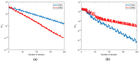
Figure 1. The comparison of two choices of ${\beta }_i^{(k)}$ for different random choices of $x^0$ for Example 1. (a) Number of iteration.

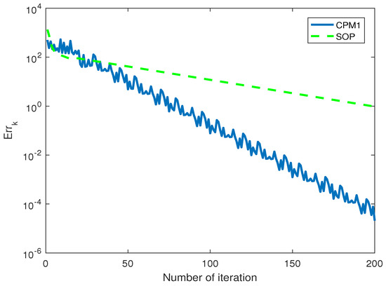
Figure 2. The comparison of the CPM and the successive orthogonal projection method (SOP) for Example 1.

Example 2.

Consider the linear equation system:

$$Ax=b$$

(24)

where A is an $m\times n$ matrix, $m<n$, and b is a vector in $R^m.$ If the noise is taken into consideration, Problem (24) is stated as

$${\parallel Ax-b\parallel }^2\le ϵ$$

(25)

where $ϵ>0$ measures the level of errors.

Let

$$C^i=\{x\in {\mathbb{R}}^n\mid |⟨A(i,:),x⟩-b(i)|-{ϵ}_i\le 0\}.$$

where ${ϵ}_i\ge 0$. It is easy to show that Problem (25) is equal to the convex feasibility problem:

$$\mathrm{Find}\mathrm{a}\mathrm{point}{x}^{*}\in C=\bigcap _{i=1}^m{C}^i$$

(26)

The set C is nonempty since the linear equation system has infinite solutions.

Set

$$Er{r}_k:=\underset{1\le i\le m}{max}|A(i,:)x^k-b(i)|.$$

(27)

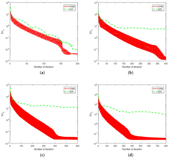
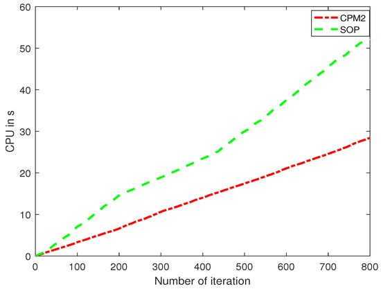
The initial point $x^0$ is randomly chosen in ${(0,10)}^n$. We compared the CPM2 and SOP for different m and n. From Figure 3, the behavior of the CPM2 is better than that of the SOP. The error of the CPM2 has a bigger oscillation than that in Example 2, the oscillation seems to decrease when the iteration is very big. The SOP behaves well when m and n are small, while its error is very big for big m and n. In Figure 4, we compare the CPU time of the CPM2 and SOP, which illustrates that the CPU time of the CPM2 is less than that of the SOP. Furthermore, the CPU time of the SOP exceeds that of the CPM2 with the iteration.

Figure 3. (a) $(m,n)$ = (20, 40); (b) $(m,n)$ = (200, 400); (c) $(m,n)$ = (500, 1000); (d) $(m,n)$ = (1000, 2000). Comparison of the CPM1 and SOP for different m and n of Example 2.

Figure 4. The comparison of the CPU time of the CPM and SOP for $(m,n)$ = (1000, 2000) of Example 2.

5. Conclusions

In this paper, we propose the combination projection method (CPM) for solving the convex feasibility problem (CFP). The CPM is simple and easy to implement, and has a fast convergence speed. How to further speed up the convergence for the CPM through selecting the convex combination coefficients ${\{{\beta }_i^{(k)}\}}_{i\in I_k}$ in Algorithms 1 and 2 is worthy of further study.

References

- Bauschke, H.H.; Borwein, J.M. On projection algorithms for solving convex feasibility problem. SIAM Rev. 1996, 38, 367–426. [Google Scholar] [CrossRef]
- Bregman, L.M. The method of successive projections for finding a common point of convex sets. Sov. Math. Dokl. 1965, 6, 688–692. [Google Scholar]
- Aleyner, A.; Reich, S. Block-iterative algorithms for solving convex feasibility problems in Hilbert and Banach spaces. J. Math. Anal. Appl. 2008, 343, 427–435. [Google Scholar] [CrossRef]
- López, G.; Martín-Márquez, V.; Wang, F.H.; Xu, H.K. Solving the split feasibility problem without prior knowledge of matrix norms. Inverse Probl. 2012, 28, 374–389. [Google Scholar] [CrossRef]
- Dong, Q.L.; Tang, Y.C.; Cho, Y.J.; Rassias, T.M. “Optimal” choice of the step length of the projection and contraction methods for solving the split feasibility problem. J. Glob. Optim. 2018, 71, 341–360. [Google Scholar] [CrossRef]
- Facchinei, F.; Pang, J.-S. Finite-Dimensional Variational Inequalities and Complementarity Problems; Springer Series in Operations Research; Springer: New York, NY, USA, 2003; Volume II. [Google Scholar]
- Dong, Q.L.; Lu, Y.Y.; Yang, J. The extragradient algorithm with inertial effects for solving the variational inequality. Optimization 2016, 65, 2217–2226. [Google Scholar] [CrossRef]
- Cegielski, A. Iterative Methods for Fixed Point Problems in Hilbert Spaces; Springer: Paris, France, 2013. [Google Scholar]
- Fukushima, M. A relaxed projection method for variational inequalities. Math. Programs 1986, 35, 58–70. [Google Scholar] [CrossRef]
- He, S.; Zhao, Z.; Luo, B. A relaxed self-adaptive CQ algorithm for the multiple-sets split feasibility problem. Optimization 2015, 64, 1907–1918. [Google Scholar] [CrossRef]
- He, H.; Xu, H.K. Splitting methods for split feasibility problems with application to Dantzig selectors. Inverse Probl. 2017, 33, 055003. [Google Scholar] [CrossRef]
- Gibali, A.; Censor, Y.; Reich, S. The subgradient extragradient method for solving variational inequalities in in Hilbert space. J. Optim. Anal. Theory Appl. 2011, 148, 318–335. [Google Scholar]
- He, S.; Yang, C. Solving the variational inequality problem defined on intersection of finite level sets. Abstr. Appl. Anal. 2013, 2013, 942315. [Google Scholar] [CrossRef]
- von Neumann, J. Functional Operators, Volume II: The Geometry of Orthogonal Spaces. In Annals of Mathematical Studies; Reprint of 1933 Lecture Notes; Princeton University Press: Princeton, NJ, USA, 1950; Volume 22. [Google Scholar]
- Zaslavski, A.J. Approximate Solutions of Common Fixed-Point Problems; Springer: New York, NY, USA, 2018. [Google Scholar]
- Combettes, P.L. The convex feasibility problem in image recovery. In Advances in Imaging and Electron Physics; Hawkes, P., Ed.; Academic Press: New York, NY, USA, 1996; Volume 95, pp. 155–270. [Google Scholar]
- Censor, Y.; Gibali, A.; Lenzen, F.; Schnörr, C. The implicit convex feasibility problem and its application to adaptive image denoising. J. Comput. Math. 2016, 34, 1–16. [Google Scholar] [CrossRef]
- Censor, Y.; Elfving, T.; Kopf, N.; Bortfeld, T. The multiple-sets split feasibility problem and its applications for inverse problem. Inverse Probl. 2005, 21, 2071–2084. [Google Scholar] [CrossRef]
- Boyd, S.; Parikh, N.; Chu, E.; Peleato, B.; Eckstein, J. Distributed optimization and statistical learning via the alternating direction method of multipliers. Found. Trends Mach. Learn. 2011, 3, 1–122. [Google Scholar] [CrossRef]
- Zhao, X.; Ng, K.F.; Li, C.; Yao, Y.C. Linear regularity and linear convergence of projection-based methods for solving convex feasibility problems. Appl. Math. Opt. 2018, 78, 613–641. [Google Scholar] [CrossRef]
- Burachik, R.S.; Martín-Márquez, V. An approach for the convex feasibility problem via monotropic programming. J. Math. Anal. Appl. 2017, 453, 746–760. [Google Scholar] [CrossRef]
- Gibali, A.; Küfer, K.-H.; Reem, D.; Süss, P. A generalized projection-based scheme for solving convex constrained optimization problems. Comput. Optim. Appl. 2018, 70, 737–762. [Google Scholar] [CrossRef]
- Aragón Artachoa, F.J.; Censor, Y.; Gibali, A. The cyclic Douglas-Rachford algorithm with r-sets-DouglasCRachford operators. Optim. Method Softw. 2018. [Google Scholar] [CrossRef]
- Censor, Y.; Zenios, S.A. Parallel Optimization: Theory, Algorithm, and Applications; Oxdord University Press: New York, NY, USA, 1997. [Google Scholar]
- Hundal, H.S. An alternating projection that does not converge in norm. Nonlinear Anal. 2004, 57, 35–61. [Google Scholar] [CrossRef]
- Gubin, L.G.; Polyak, B.T.; Raik, E.V. The method of projections for finding the common point of convex sets. USSR Comput. Math. Math. Phys. 1967, 7, 1–24. [Google Scholar] [CrossRef]
- Bruck, R.E.; Reich, S. Nonexpansive projections and resolvents of accretive operators in Banach spaces. Houst. J. Math. 1977, 3, 459–470. [Google Scholar]
- He, S.; Zhao, Z.; Luo, B. A simple algorithm for computing projection onto intersection of finite level sets. J. Inequal. Appl. 2014, 2014, 307. [Google Scholar] [CrossRef]
- He, S.; Tian, H. Selective projection methods for solving a class of variational inequalities. Numer. Algorithms 2018, 1–18. [Google Scholar] [CrossRef]
- He, S.; Tian, H.; Xu, H.K. The selective projection method for convex feasibility and split feasibility problems. J. Nonlinear Convex Anal. 2018, 19, 1199–1215. [Google Scholar]
- Xu, H.K. Averaged mappings and the gradient-projection algorithm. J. Optim. Theory Appl. 2011, 150, 360–378. [Google Scholar] [CrossRef]
- López Acedo, G.; Xu, H.K. Iterative methods for strict pseudo-contractions in Hilbert spaces. Nonlinear Anal. 2007, 67, 2258–2271. [Google Scholar] [CrossRef]
© 2018 by the authors. Licensee MDPI, Basel, Switzerland. This article is an open access article distributed under the terms and conditions of the Creative Commons Attribution (CC BY) license (http://creativecommons.org/licenses/by/4.0/).