Global Dynamics of Certain Mix Monotone Difference Equation

Abstract

We investigate global dynamics of the following second order rational difference equation $x_{n+1}=\frac{x_n{x}_{n-1}+\alpha x_n+\beta x_{n-1}}{a{x}_n{x}_{n-1}+b{x}_{n-1}},$ where the parameters $\alpha ,\beta ,a,b$ are positive real numbers and initial conditions $x_{-1}$ and $x_0$ are arbitrary positive real numbers. The map associated to the right-hand side of this equation is always decreasing in the second variable and can be either increasing or decreasing in the first variable depending on the corresponding parametric space. In most cases, we prove that local asymptotic stability of the unique equilibrium point implies global asymptotic stability.

1. Introduction and Preliminaries

In this paper, we investigate the local and global character of the equilibrium point of the following second order rational difference equation

$$x_{n+1}=\frac{x_n{x}_{n-1}+\alpha x_n+\beta x_{n-1}}{a{x}_n{x}_{n-1}+b{x}_{n-1}},n=0,1,\dots$$

(1)

where the parameters $\alpha ,\beta ,a,b$ are nonnegative real numbers and initial conditions $x_{-1}$ and $x_0$ are arbitrary nonnegative real numbers, such that $a{x}_n{x}_{n-1}+b{x}_{n-1}>0$, $n=0,1,\dots$.

Equation (1) is the special case of a general second order quadratic rational difference equation of the form

$$x_{n+1}=\frac{A{x}_n^2+B{x}_n{x}_{n-1}+C{x}_{n-1}^2+D{x}_n+E{x}_{n-1}+F}{a{x}_n^2+b{x}_n{x}_{n-1}+c{x}_{n-1}^2+d{x}_n+e{x}_{n-1}+f},n=0,1,\dots$$

(2)

with nonnegative parameters and nonegative initial conditions such that $A+B+C>0$, $a+b+c+d+e+f>0$ and $a{x}_n^2+b{x}_n{x}_{n-1}+c{x}_{n-1}^2+d{x}_n+e{x}_{n-1}+f>0$, $n=0,1,\dots$. Several global asymptotic results for some special cases of Equation (2) were obtained in [1,2,3,4,5,6,7,8,9,10,11].

One interesting special case by (2) is the following rational difference equation studied in [12]:

$$x_{n+1}=\frac{D{x}_n+F}{d{x}_n+e{x}_{n-1}},n=0,1,\dots$$

(3)

which represents discretization of the differential equation model in biochemical networks, see [13]. Notice that Equation (3) is an example of a rational difference equation, such that associated map is always strictly decreasing with respect to the second variable, and changes its monotonicity with respect to the first variable, i.e., can be increasing or decreasing depending on corresponding parametric space. Also, we see that Equation (3) is the special case of the linear rational difference equation

$$x_{n+1}=\frac{D{x}_n+E{x}_{n-1}+F}{d{x}_n+e{x}_{n-1}+f},n=0,1,\dots$$

(4)

(which was investigated in detail in [12]) with well known and complicated dynamics, such as Lynes’ equation (see [14]).

There are not many papers that study in detail dynamics of the second order rational difference equations with quadratic terms such that associated map changes its monotonicity with respect to its variables. However, in [15] the behavior of the following rational difference equation has been investigated in great detail

$$x_{n+1}=\frac{\alpha +\gamma x_{n-1}}{B{x}_n+D{x}_n{x}_{n-1}+x_{n-1}},n=0,1,\dots$$

(5)

In both equations, (3) and (5), Theorems 1 and 2 were used in order to obtain the convergence results. In most cases of this paper we use the same results. However, in order to investigate the behaviour of the following four subsequences ${\left\{x_{4k}\right\}}_{k=1}^{\infty }$, ${\left\{x_{4k+1}\right\}}_{k=0}^{\infty }$, ${\left\{x_{4k+2}\right\}}_{k=0}^{\infty }$, ${\left\{x_{4k+3}\right\}}_{k=0}^{\infty }$ that appears under the condition $\frac{b\alpha }{a\beta -b}=\frac{\beta }{b},$ where $\beta >\frac{b}{a}$ we cannot use this method, because the associated map in this case does not have the same monotonicity with respect to its variables in invariant interval. More precisely, the corresponding map changes its monotonicity in invariant interval with respect to the first variable. Instead of that, we use the brute-force method to show that each subsequence converges to the unique equilibrium point.

In the case when associated map of Equation (1) changes its monotonicity from “decreasing-decreasing” into “increasing-decreasing”, the problem of determining invariant interval appears. In all cases, we determine invariant interval and prove that the positive equilibrium of Equation (1), which is always locally asymptotically stable, is globally asymptotically stable for all values of the parameters, except in the case when $\alpha >{\alpha }_D$ (see Theorems 7–10).

The problem of determining invariant intervals in the case when the associated map changes its monotonicity with respect to its variables has been considered in [16,17]. Also, see [18,19,20].

Now, we state several well-known results.

Theorem 1.

[14] [Theorem 2.22] Let $\left[a,b\right]$ be an interval, and suppose that $f:\left[a,b\right]\times \left[a,b\right]\to \left[a,b\right]$ is a continuous function. Consider the difference equation

$$x_{n+1}=f\left(x_n,x_{n-1}\right),n=0,1,\dots$$

(6)

Assume that f satisfies the following two conditions:

a. $f\left(x,y\right)$ is nondecreasing in $x\in \left[a,b\right]$ for each $y\in \left[a,b\right]$, and $f\left(x,y\right)$ is nonincreasing in $y\in \left[a,b\right]$ for each $x\in \left[a,b\right]$;

b. All solutions $\left(m,M\right)\in \left[a,b\right]\times \left[a,b\right]$ of the system

$$m=f\left(m,M\right),M=f\left(M,m\right)$$

satisfy $m=M$.

Then, (6) has a unique equilibrium $\overline{x}\in \left[a,b\right]$ and every solution of (6) converges to $\overline{x}.$

Theorem 2.

[12] [Theorem 1.4.7] Let $\left[a,b\right]$ be an interval, and suppose that $f:\left[a,b\right]\times \left[a,b\right]\to \left[a,b\right]$ is a continuous function satisfying the following properties:

a. $f\left(x,y\right)$ is nonincreasing in each of its arguments;

b. If $\left(m,M\right)\in \left[a,b\right]\times \left[a,b\right]$ is a solution of the system

$$m=f\left(M,M\right),M=f\left(m,m\right),$$

then $m=M$.

Then, (6) has a unique equilibrium $\overline{x}\in \left[a,b\right]$ and every solution of (6) converges to $\overline{x}.$

Theorem 3.

[21] [Theorem 1.4] Let f be the function from (6) with

1. 

$f\in C\left[\left(0,\infty \right)\times \left(0,\infty \right),\left(0,\infty \right)\right]$;

2. 

$f\left(u,v\right)$ is nonincreasing in u and v respectively;

3. 

$xf\left(x,x\right)$ is nondecreasing in x;

4. 

Equation (6) has a unique positive equilibrium $\overline{x}$.

Then, every positive solution ${\left\{x_n\right\}}_{n=-1}^{\infty }$ of Equation (6) which is bounded from above and from below by positive constants converges to $\overline{x}$.

Theorem 4.

[12] [Theorem 1.7.2] Assume that $f\in C\left[\left(0,\infty \right)\times \left(0,\infty \right),\left(0,\infty \right)\right]$ and that $f\left(x,y\right)$ is decreasing in both arguments.

Let $\overline{x}$ be a positive equilibrium of Equation (6). Then, every oscillatory solution of Equation (6) has semicycles of length at most two.

Theorem 5.

[12] [Theorem 1.7.4] Assume that $f\in C\left[\left(0,\infty \right)\times \left(0,\infty \right),\left(0,\infty \right)\right]$ is such that: $f\left(x,y\right)$ is increasing in x for each fixed y, and $f\left(x,y\right)$ is decreasing in y for each fixed x.

Let $\overline{x}$ be a positive equilibrium of Equation (6). Then, except for the first semicycle, every oscillatory solution of Equation (6) has semicycles of length at least two.

2. Linearized Stability

In this section, we prove that Equation (1) has a unique equilibrium point which is always locally asymptotically stable.

The equilibrium point $\overline{x}$ of Equation (1) satisfies

$$\overline{x}=\frac{{\overline{x}}^2+\alpha \overline{x}+\beta \overline{x}}{a{\overline{x}}^2+b\overline{x}}.$$

(7)

Equation (7) has the unique positive solution

$$\overline{x}=\frac{1-b+\sqrt{D}}{2a},$$

(8)

where

$$D={(b-1)}^2+4a(\alpha +\beta ).$$

Theorem 6.

The unique positive Equilibrium (8) of Equation (1) is always locally asymptotically stable.

Proof. 

The real function $f(u,v)$ associated to Equation (1) is given by

$$f(u,v)=\frac{uv+\alpha u+\beta v}{auv+bv}.$$

Derivatives with respect to u and v evaluated at the equilibrium point (8) are respectively

$$p=\frac{b\alpha +(b-a\beta )\overline{x}}{(\overline{x}+\alpha +\beta )(b+a\overline{x})},\mathrm{and}q=-\frac{\alpha }{\overline{x}+\alpha +\beta }.$$

We have that the function $f(u,v)$ is always decreasing with respect to the second variable and can be either decreasing or increasing with respect to the first variable, depending on the sign of nominator, that is depending on corresponding parametric space. Now, we check the conditions of Theorem 1.1.1, see [12]. The condition $\left|p\right|<1-q<2$ becomes

$$\left|\frac{b\alpha +(b-a\beta )\overline{x}}{(\overline{x}+\alpha +\beta )(b+a\overline{x})}\right|<1+\frac{\alpha }{\overline{x}+\alpha +\beta }<2.$$

The second inequality is equivalent to $\alpha <\overline{x}+\alpha +\beta$, which is always true. The first inequality becomes

$$-\left(1+\frac{\alpha }{\overline{x}+\alpha +\beta }\right)<\frac{b\alpha +(b-a\beta )\overline{x}}{(\overline{x}+\alpha +\beta )(b+a\overline{x})}<1+\frac{\alpha }{\overline{x}+\alpha +\beta }.$$

Now, we have

$$-\left(1+\frac{\alpha }{\overline{x}+\alpha +\beta }\right)<\frac{b\alpha +(b-a\beta )\overline{x}}{(\overline{x}+\alpha +\beta )(b+a\overline{x})}\iff -\frac{3b\alpha +b\beta +a{\overline{x}}^2+2b\overline{x}+2a\alpha \overline{x}}{(\overline{x}+\alpha +\beta )(b+a\overline{x})}<0,$$

which is always true.

Also, we have

$$\frac{b\alpha +(b-a\beta )\overline{x}}{(\overline{x}+\alpha +\beta )(b+a\overline{x})}<1+\frac{\alpha }{\overline{x}+\alpha +\beta }\iff -\frac{b\alpha +b\beta +a{\overline{x}}^2+2a\alpha \overline{x}+2a\overline{x}\beta }{(\overline{x}+\alpha +\beta )(b+a\overline{x})}<0,$$

which is always true. □

Lemma 1.

Every solution of Equation (1) is bounded.

Proof. 

From Equation (1), we have

$$\begin{array}{cc}\hfill x_{n+1}& =\frac{x_n{x}_{n-1}+\alpha x_n+\beta x_{n-1}}{a{x}_n{x}_{n-1}+b{x}_{n-1}}\ge \frac{x_n{x}_{n-1}+\beta x_{n-1}}{a{x}_n{x}_{n-1}+b{x}_{n-1}}\ge min\left\{\frac{1}{a},\frac{\beta }{b}\right\},\hfill \\ \hfill x_{n+1}& =\frac{x_n{x}_{n-1}+\alpha x_n+\beta x_{n-1}}{a{x}_n{x}_{n-1}+b{x}_{n-1}}=\frac{\alpha x_n}{a{x}_n{x}_{n-1}+b{x}_{n-1}}+\frac{x_n{x}_{n-1}+\beta x_{n-1}}{a{x}_n{x}_{n-1}+b{x}_{n-1}},\hfill \\ \hfill x_{n+1}& \le \frac{\alpha x_n}{a{x}_n{x}_{n-1}}+max\left\{\frac{1}{a},\frac{\beta }{b}\right\},\hfill \\ \hfill x_{n+1}& \le \frac{\alpha }{a{x}_{n-1}}+max\left\{\frac{1}{a},\frac{\beta }{b}\right\}\le \left\{\begin{array}{cc}\alpha +\frac{\beta }{b},\hfill & \frac{1}{a}<\frac{\beta }{b}\hfill \\ \frac{\alpha b}{\beta a}+\frac{1}{a},\hfill & \frac{1}{a}>\frac{\beta }{b}\hfill \\ \alpha +\frac{1}{a},\hfill & \frac{1}{a}=\frac{\beta }{b}\hfill \end{array}\right.\hfill \end{array}$$

which completes the proof. □

Lemma 2.

Equation (1) does not posses a minimal period-two solution.

Proof. 

Period-two solution $(x,y),x>0,y>0,x\ne y,$ satisfies the following system of algebraic equations

$$\begin{array}{cc}\hfill x-f(y,x)& =0\hfill \\ \hfill y-f(x,y)& =0.\hfill \end{array}$$

(9)

By replacing the function $f,$ we have

$$\begin{array}{cc}\hfill a{x}^{2}y+b{x}^2-\beta x-xy-\alpha y& =0\hfill \\ \hfill ax{y}^2+b{y}^2-\alpha x-xy-\beta y& =0.\hfill \end{array}$$

(10)

By subtracting these two equations, we obtain

$$\left(x-y\right)\left[axy+b\left(x+y\right)+\alpha -\beta \right]=0.$$

If $\alpha \ge \beta$, then there does not exist a minimal period-two solution. However, if $\alpha <\beta$, we have

$$axy+b\left(x+y\right)=\beta -\alpha .$$

(11)

Similarly, by adding, from (10) we obtain

$$\left(x+y\right)\left[axy+b\left(x+y\right)-\alpha -\beta \right]=2xy\left(1+b\right),$$

from which

$$axy+b\left(x+y\right)-\alpha -\beta >0.$$

(12)

By using (11), we have

$$axy+b\left(x+y\right)-\alpha -\beta =\beta -\alpha -\alpha -\beta =-2\alpha <0,$$

which is a contradiction with (12). ☐

3. Global Attractivity Results

In this section, we prove several global attractivity results in the corresponding parametric space.

We notice that the sign of the partial derivative with respect to the first variable at the equilibrium point depends on the sign of the $b-a\beta$.

$b-a\beta \ge 0$, In this case, the function f is increasing in the first variable and decreasing in the second variable.

Lemma 3.

If $\alpha \le \beta$ or $\alpha >\beta ,b\le 1$ or $\beta <\alpha \le {\alpha }_D=\frac{4a{\beta }^2}{{\left(b-1\right)}^2}+\beta ,b>1$, then the system of algebraic equations

$$m=f\left(m,M\right),M=f\left(M,m\right)$$

(13)

has a unique solution $\left(m,M\right)=\left(\overline{x},\overline{x}\right)$.

Proof. 

System (13) is of the form

$$m=\frac{M\beta +m\alpha +Mm}{M\left(b+am\right)},M=\frac{M\alpha +m\beta +Mm}{m\left(b+Ma\right)},$$

that is

$$\begin{array}{cc}\hfill M\beta +m\alpha +Mm& =mM\left(b+am\right),\hfill \end{array}$$

(14)

$$\begin{array}{cc}\hfill M\alpha +m\beta +Mm& =Mm\left(b+Ma\right).\hfill \end{array}$$

(15)

By subtracting Equations (14) and (15), we obtain

$$\left(m-M\right)\left(amM-\alpha +\beta \right)=0.$$

If $\alpha \le \beta$, then system (13) has a unique solution $\left(m,M\right)=\left(\overline{x},\overline{x}\right)$.

Suppose that $\alpha >\beta$ and $M\ne m$. Then

$$M=\frac{\alpha -\beta }{am}.$$

(16)

By adding Equations (14) and (15), we have

$$\left(m+M\right)\left(amM-\alpha -\beta \right)=2\left(1-b\right)mM,$$

from which, by using (16), we have

$$\beta \left(m+M\right)=\left(b-1\right)mM.$$

(17)

Now, we see that Equation (17) has no positive solutions $\left(m,M\right)$ if $b\le 1.$ This means that system (13) has a unique solution $\left(m,M\right)=\left(\overline{x},\overline{x}\right)$ in this case.

Assume that $b>1$. By substituting (16) into (17) we obtain quadratic equation

$$a\beta m^2-\left(b-1\right)\left(\alpha -\beta \right)m+\beta \left(\alpha -\beta \right)=0,$$

with solutions

$$m_{\pm }=\frac{\left(b-1\right)\left(\alpha -\beta \right)\pm \sqrt{\left(\alpha -\beta \right)\left[{\left(b-1\right)}^2\left(\alpha -\beta \right)-4a{\beta }^2\right]}}{2a\beta }.$$

It is easy to see that $m_{\pm }\notin \mathbb{R}$ when $\alpha <\frac{4a{\beta }^2}{{\left(b-1\right)}^2}+\beta ={\alpha }_D$, which means that system (13) has a unique solution $\left(m,M\right)=\left(\overline{x},\overline{x}\right)$ in this case. Similarly, if $\alpha ={\alpha }_D$, then $m=M=\frac{2\beta }{b-1}=\overline{x}$.

Finally, if $\alpha >{\alpha }_D$, then system (13) has more than one positive solution. □

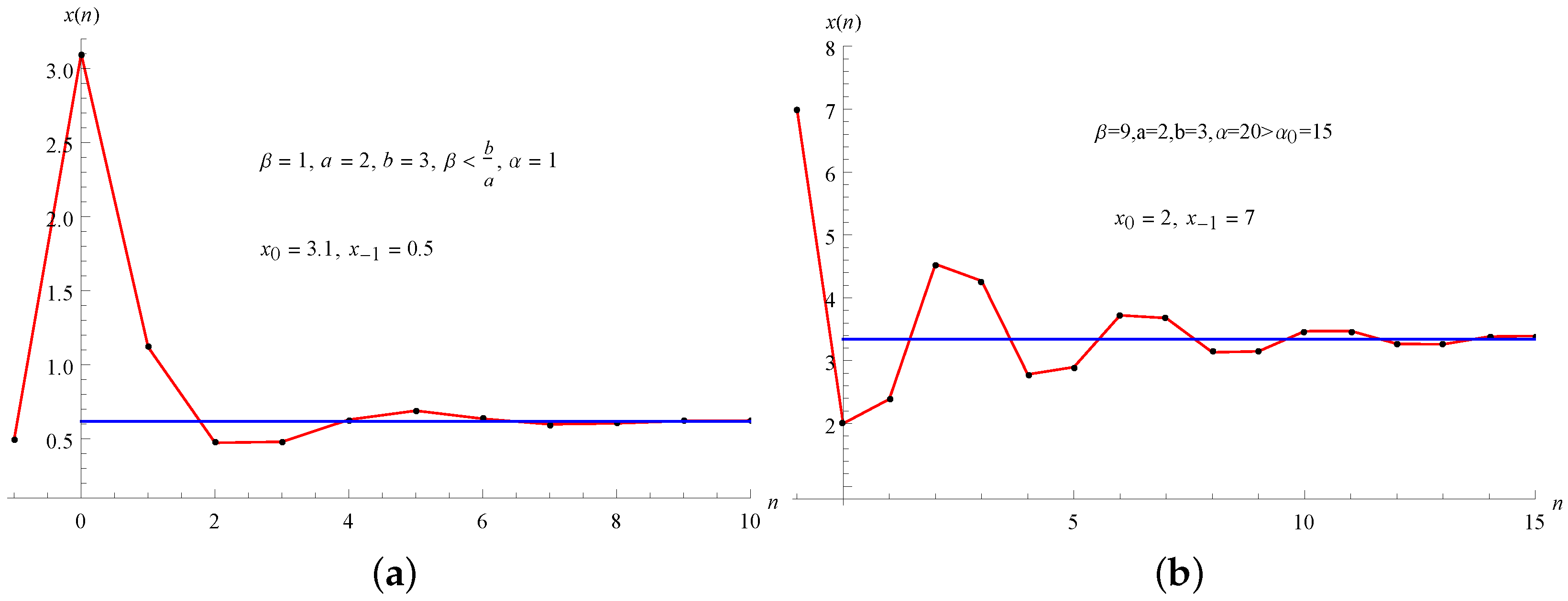
Theorem 7.

Assume that one of the following conditions hold:

(1) 

$1\ge b\ge a\beta ,$$\left(\alpha >0,a>0\right),$

(2) 

$b>1,b\ge a\beta ,\alpha \le {\alpha }_D,$$\left(a>0\right).$

Then, the unique Equilibrium (8) of Equation (1) is globally asymptotically stable.

Proof. 

In this case (see the proof of Lemma 1) the invariant interval (and an attracting interval) of Equation (1) is

$$\left[\frac{1}{a},\frac{\beta }{b}+\alpha \right].$$

Since ${\displaystyle \frac{\partial f(u,v)}{\partial u}}={\displaystyle \frac{b\alpha +(b-a\beta )v}{v{(b+au)}^2}}>0$, then f is increasing in the first variable and decreasing in the second variable and we can apply Theorem 1. Also, we know that the equilibrium $\overline{x}$ is locally asymptotically stable, and consequently the proof will be completed by using Lemma 3 and Theorem 1. □

For some numerical values of parameters we give visual evidence for Theorem 7. (See Figure 1a).

Figure 1. Numerical simulation of stability for: (a) $b-a\beta \ge 0$; (b) $b-a\beta <0$ and $v_0>{\displaystyle \frac{\beta }{b}}$.

$b-a\beta <0$, Lemma 1 implies that

$$\frac{1}{a}\le x_{n+1}\le \alpha +\frac{\beta }{b}.$$

Now, we have

$$\frac{\partial f(u,v)}{\partial u}=\frac{b\alpha +(b-a\beta )v}{v{(b+au)}^2}\left\{\begin{array}{cc}=0,\hfill & v=v_0=\frac{b\alpha }{a\beta -b},\hfill \\ >0,\hfill & v<v_0=\frac{b\alpha }{a\beta -b},\hfill \\ <0,\hfill & v>v_0=\frac{b\alpha }{a\beta -b}.\hfill \end{array}\right.$$

Since

$$f\left(\frac{b\alpha }{a\beta -b},\frac{b\alpha }{a\beta -b}\right)=\frac{\beta }{b},$$

we have to consider the following three cases:

(i)

$v_0={\displaystyle \frac{b\alpha }{a\beta -b}}>{\displaystyle \frac{\beta }{b}},$

(ii)

$v_0={\displaystyle \frac{b\alpha }{a\beta -b}}={\displaystyle \frac{\beta }{b}},$

(iii)

$v_0={\displaystyle \frac{b\alpha }{a\beta -b}}<{\displaystyle \frac{\beta }{b}}.$

For the case of $v_0={\displaystyle \frac{b\alpha }{a\beta -b}}>{\displaystyle \frac{\beta }{b}}$ we have the following result about global behavior of solutions of Equation (1).

Theorem 8.

Assume that one of the following conditions hold:

(1) 

$b\le 1,\beta >{\displaystyle \frac{b}{a}}$$\left(\alpha >{\alpha }_0,a>0\right),$

(2) 

$b>1,\beta >{\displaystyle \frac{b}{a}},{\alpha }_0<\alpha \le {\alpha }_D,$$\left(a>0\right),$

where ${\alpha }_0={\displaystyle \frac{\beta \left(a\beta -b\right)}{b^2}}.$ Then, the unique Equilibrium (8) of Equation (1) is globally asymptotically stable.

Proof. 

Since $v_0={\displaystyle \frac{b\alpha }{a\beta -b}}>{\displaystyle \frac{\beta }{b}}$, we have that ${\displaystyle \frac{b\alpha }{a\beta -b}}-{\displaystyle \frac{\beta }{b}}={\displaystyle \frac{b\beta -a{\beta }^2+b^2\alpha }{b\left(a\beta -b\right)}}>0$, i.e., $b\beta -a{\beta }^2+b^2\alpha >0,$ from which $\alpha >{\alpha }_0={\displaystyle \frac{\beta \left(a\beta -b\right)}{b^2}},\beta >{\displaystyle \frac{b}{a}}.$

In this case we have

$$f:{\left[{\displaystyle \frac{\beta }{b}},{\displaystyle \frac{b\alpha }{a\beta -b}}\right]}^2\to \left[{\displaystyle \frac{\beta }{b}},{\displaystyle \frac{b\alpha }{a\beta -b}}\right],$$

which implies that the interval $\left[{\displaystyle \frac{\beta }{b}},{\displaystyle \frac{b\alpha }{a\beta -b}}\right]$ is an invariant interval. Indeed, since the function $f(u,v)$ is continuous, then $f(u,v)$ attains its extreme points at the end of closed interval or at the stationary point. Straightforward calculations show that all values

$$f\left({\displaystyle \frac{b\alpha }{a\beta -b}},{\displaystyle \frac{b\alpha }{a\beta -b}}\right)={\displaystyle \frac{\beta }{b}},f\left({\displaystyle \frac{\beta }{b}},{\displaystyle \frac{b\alpha }{a\beta -b}}\right)={\displaystyle \frac{\beta }{b}},$$

$$f\left({\displaystyle \frac{b\alpha }{a\beta -b}},{\displaystyle \frac{\beta }{b}}\right)={\displaystyle \frac{b^2{\alpha }^2+b\alpha \beta -b{\beta }^2+a{\beta }^3}{b\beta \left(a\alpha +a\beta -b\right)}},f\left({\displaystyle \frac{\beta }{b}},{\displaystyle \frac{\beta }{b}}\right)={\displaystyle \frac{\beta +b\alpha +b\beta }{b^2+a\beta }}$$

are in $\left[{\displaystyle \frac{\beta }{b}},{\displaystyle \frac{b\alpha }{a\beta -b}}\right].$

Set

$$g\left(x\right)=a{x}^2+(b-1)x-\alpha -\beta .$$

We know that $g\left(\overline{x}\right)=0.$ On the other hand, we have that

$$g\left({\displaystyle \frac{\beta }{b}}\right)=-{\displaystyle \frac{b\beta -a{\beta }^2+b^2\alpha }{b^2}}<0,g\left({\displaystyle \frac{b\alpha }{a\beta -b}}\right)=\frac{\left(a\alpha +a\beta -b\right)\left(b\beta -a{\beta }^2+b^2\alpha \right)}{{\left(a\beta -b\right)}^2}>0,$$

which implies $\overline{x}\in \left[{\displaystyle \frac{\beta }{b}},{\displaystyle \frac{b\alpha }{a\beta -b}}\right]$.

Also, we know that ${\displaystyle \frac{\partial f(u,v)}{\partial u}}={\displaystyle \frac{b\alpha +(b-a\beta )v}{v{(b+au)}^2}}>0$, which implies that f is increasing in the first variable and decreasing in the second variable. Since Equation (1) has the unique equilibrium point in invariant interval $\left[{\displaystyle \frac{\beta }{b}},{\displaystyle \frac{b\alpha }{a\beta -b}}\right]$, we can apply Theorem 1. Also, we know that the equilibrium $\overline{x}$ is locally asymptotically stable, and consequently the proof will be completed by using Lemma 3 and Theorem 1. □

For some numerical values of parameters we give visual evidence for Theorem 8. (See Figure 1b).

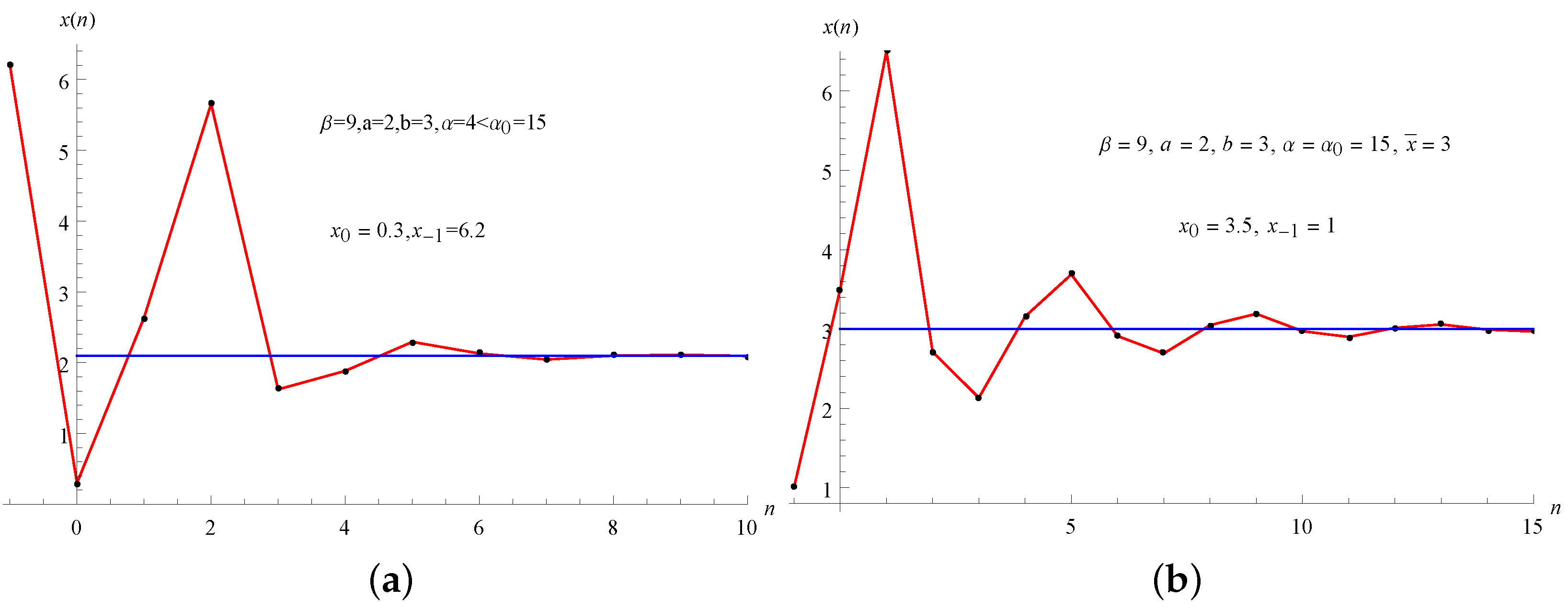
For the case of $v_0={\displaystyle \frac{b\alpha }{a\beta -b}}<{\displaystyle \frac{\beta }{b}}$ the following result holds.

Theorem 9.

Assume that $v_0={\displaystyle \frac{b\alpha }{a\beta -b}}<{\displaystyle \frac{\beta }{b}}.$ Then, the invariant interval of Equation (1) is

$$\left[\frac{b\alpha }{a\beta -b},\frac{\beta }{b}\right],$$

that is

$$f:{\left[\frac{b\alpha }{a\beta -b},\frac{\beta }{b}\right]}^2\to \left[\frac{b\alpha }{a\beta -b},\frac{\beta }{b}\right]$$

and the unique Equilibrium (8) of Equation (1) is globally asymptotically stable.

Proof. 

Since $v_0={\displaystyle \frac{b\alpha }{a\beta -b}}<{\displaystyle \frac{\beta }{b}}$, then ${\displaystyle \frac{b\alpha }{a\beta -b}}-{\displaystyle \frac{\beta }{b}}={\displaystyle \frac{b\beta -a{\beta }^2+b^2\alpha }{b\left(a\beta -b\right)}}<0$, that is $b\beta -a{\beta }^2+b^2\alpha <0$, from which $\alpha <{\alpha }_0={\displaystyle \frac{\beta \left(a\beta -b\right)}{b^2}},\beta >{\displaystyle \frac{b}{a}}$.

First, we prove that the invariant interval is given by $\left[{\displaystyle \frac{b\alpha }{a\beta -b}},{\displaystyle \frac{\beta }{b}}\right]$. Since the function $f(u,v)$ is continuous, then this function attains its extreme points at the end of closed interval or at the stationary point. Straightforward calculations show that

$$f\left(\frac{b\alpha }{a\beta -b},\frac{b\alpha }{a\beta -b}\right)=\frac{\beta }{b},f\left(\frac{\beta }{b},\frac{b\alpha }{a\beta -b}\right)=\frac{\beta }{b},$$

$$f\left(\frac{b\alpha }{a\beta -b},\frac{\beta }{b}\right)={\displaystyle \frac{b^2{\alpha }^2+b\alpha \beta -b{\beta }^2+a{\beta }^3}{b\beta \left(a\alpha +a\beta -b\right)}},f\left(\frac{\beta }{b},\frac{\beta }{b}\right)={\displaystyle \frac{\beta +b\alpha +b\beta }{b^2+a\beta }}$$

are in $\left[{\displaystyle \frac{b\alpha }{a\beta -b}},{\displaystyle \frac{\beta }{b}}\right]$.

Now, we prove that the equilibrium point is in interval $\left[{\displaystyle \frac{b\alpha }{a\beta -b}},{\displaystyle \frac{\beta }{b}}\right]$. Set

$$g\left(x\right)=a{x}^2+(b-1)x-\alpha -\beta .$$

We know that $g\left(\overline{x}\right)=0.$ On the other hand, we have

$$g\left(\frac{\beta }{b}\right)=-\frac{b\beta -a{\beta }^2+b^2\alpha }{b^2}>0,g\left(\frac{b\alpha }{a\beta -b}\right)=\frac{(a\alpha +a\beta -b)\left(b\beta -a{\beta }^2+b^2\alpha \right)}{{(a\beta -b)}^2}<0,$$

which shows that $\overline{x}\in \left[{\displaystyle \frac{b\alpha }{a\beta -b}},{\displaystyle \frac{\beta }{b}}\right]$.

Since the function $f(u,v)$ is decreasing in both variables, and Equation (1) has the unique equilibrium point in invariant interval $\left[{\displaystyle \frac{b\alpha }{a\beta -b}},{\displaystyle \frac{\beta }{b}}\right]$, we can apply Theorem 2. System of algebraic equations

$$f(M,M)=m,f(m,m)=M$$

becomes

$$\frac{M+\alpha +\beta }{b+aM}=m,\frac{m+\alpha +\beta }{b+am}=M.$$

It is easy to see that this system has a unique solution $m=M$, which completes the proof. □

For some numerical values of parameters we give visual evidence for Theorem 9. (See Figure 2a).

Figure 2. Numerical simulation of stability for $b-a\beta <0$ (a) $v_0<{\displaystyle \frac{\beta }{b}}$; (b) $v_0={\displaystyle \frac{\beta }{b}}$.

Remark 1.

Notice that we can prove Theorem 9 by using Theorem 3. In this case, we have

$$\frac{1}{a}\le x_{n+1}\le \alpha +{\displaystyle \frac{\beta }{b}},n=0,1,\dots ,$$

which means that every solution ${\left\{x_n\right\}}_{n=-1}^{\infty }$ of Equation (1) is bounded from above and from below by positive constants.

Since

$$\frac{d}{dx}\left(xf\left(x,x\right)\right)={\displaystyle \frac{a{x}^2+2bx+b\alpha +b\beta }{{\left(b+ax\right)}^2}}>0,$$

and f clearly satisfies the conditions 1. and 2. of Theorem 3. Now, by using Theorem 3, we have that every solution ${\left\{x_n\right\}}_{n=-1}^{\infty }$ of Equation (1) converges to $\overline{x}$.

Now, consider the case $v_0={\displaystyle \frac{b\alpha }{a\beta -b}}={\displaystyle \frac{\beta }{b}}$.

Lemma 4.

Assume that ${\displaystyle \frac{b\alpha }{a\beta -b}}={\displaystyle \frac{\beta }{b}}$, that is $\alpha ={\alpha }_0={\displaystyle \frac{\beta \left(a\beta -b\right)}{b^2}}$, where $\beta >{\displaystyle \frac{b}{a}}$. Then, Equation (1) does not posses a minimal period-four solution.

Proof. 

Suppose the opposite, i.e., Equaiton (1) has a minimal period-four solution: $\dots x,y,z,t,x,y,z,t,\dots$, that is the following equalities hold

$$\begin{array}{cc}\hfill z& =\frac{xy+\frac{\beta \left(a\beta -b\right)}{b^2}y+\beta x}{axy+bx},\hfill \\ \hfill t& =\frac{zy+\frac{\beta \left(a\beta -b\right)}{b^2}z+\beta y}{azy+by},\hfill \\ \hfill x& =\frac{tz+\frac{\beta \left(a\beta -b\right)}{b^2}t+\beta z}{atz+bz},\hfill \\ \hfill y& =\frac{xt+\frac{\beta \left(a\beta -b\right)}{b^2}x+\beta t}{axt+bt}.\hfill \end{array}$$

By eliminating z and t we obtain

$$\left.\begin{array}{c}{\displaystyle \frac{\left(bx-\beta \right)\Phi \left(x,y,a,b,\beta \right)}{\left(b^{2}x\left(y+\beta \right)+\left(a\beta -b\right)y\beta \right)\Omega \left(x,y,a,b,\beta \right)}}=0,\\ {\displaystyle \frac{\left(by-\beta \right)\Psi \left(x,y,a,b,\beta \right)}{\left(b+ax\right)\left[\beta \left(a\beta -b\right)\left(b^{2}xy+\left(a\beta -b\right)y\beta +b^{2}x\beta +b^2{y}^2\right)+yx{b}^4\left(y+\beta +b\beta +ay\beta \right)\right]}}=0,\end{array}\right\}$$

(18)

where

$$\begin{array}{cc}\hfill \Phi \left(x,y,a,b,\beta \right)& =A{\left(a\beta -b\right)}^3+B{\left(a\beta -b\right)}^2+C\left(a\beta -b\right)+D,\hfill \\ \hfill \Psi \left(x,y,a,b,\beta \right)& =E{\left(a\beta -b\right)}^2+F\left(a\beta -b\right)+G,\hfill \\ \hfill \Omega \left(x,y,a,b,\beta \right)& =H+J\hfill \end{array}$$

$$\begin{array}{cc}\hfill A& ={\beta }^2{y}^2,\hfill \\ \hfill B& =\beta yb\left(\left(1+a\beta \right)b{y}^2+\left(b+a\beta \right)xy+\left(b+a\beta \right)x\beta \right),\hfill \\ \hfill C& =x{b}^3\left(\left(b+a\beta +3ab\beta +a{b}^2\beta \right)y^3+\left(b+ax+a\beta +b^2+b^3+2ab\beta \right)\beta y^2+\left(2y+\beta \right)xa{\beta }^2\right),\hfill \\ \hfill D& =y{x}^2{b}^5\left(y+\beta \right)\left(ay+a\beta +aby+2ab\beta +b^3+a{b}^{2}y+a^{2}y\beta \right),\hfill \\ \hfill E& =y\beta \left(x+\beta \right),\hfill \\ \hfill F& =b\left(\left(ax+b\right)y^2\beta +\left(x+\beta \right)\left(y+\beta \right)bx\right),\hfill \\ \hfill G& =b^{3}xy\left(y+\beta +b\beta +ay\beta \right)\left(b+ax\right)\hfill \\ \hfill H& =\beta a\left(a\beta -b\right)\left(\left(a\beta -b\right)y\beta +b^2\left(\left(y+\beta \right)x+\left(1+b\right)y^2\right)\right)\hfill \\ \hfill J& =yx{b}^4\left(\left(y+\beta \right)a+ay\left(b^2+b+a\beta \right)+2ab\beta +b^3\right).\hfill \end{array}$$

Since $a\beta -b>0$, we have that $\Phi \left(x,y,a,b,\beta \right)>0$ and $\Psi \left(x,y,a,b,\beta \right)>0$. Therefore, system (18) has a unique solution of the form

$$x=\frac{\beta }{b},y=\frac{\beta }{b},$$

$$\begin{array}{cc}\hfill z& =\frac{xy+\frac{\beta \left(a\beta -b\right)}{b^2}y+\beta x}{axy+bx}=\frac{{\left(\frac{\beta }{b}\right)}^2+\frac{\beta \left(a\beta -b\right)}{b^2}\left(\frac{\beta }{b}\right)+\beta \left(\frac{\beta }{b}\right)}{a{\left(\frac{\beta }{b}\right)}^2+b\left(\frac{\beta }{b}\right)}=\frac{\beta }{b},\hfill \\ \hfill t& =\frac{zy+\frac{\beta \left(a\beta -b\right)}{b^2}z+\beta y}{azy+by}=\frac{{\left(\frac{\beta }{b}\right)}^2+\frac{\beta \left(a\beta -b\right)}{b^2}\left(\frac{\beta }{b}\right)+\beta \left(\frac{\beta }{b}\right)}{a{\left(\frac{\beta }{b}\right)}^2+b\left(\frac{\beta }{b}\right)}=\frac{\beta }{b},\hfill \end{array}$$

which means that Equaiton (1) has no a minimal period-four solution. □

Theorem 10.

Assume that ${\displaystyle \frac{b\alpha }{a\beta -b}}={\displaystyle \frac{\beta }{b}}$, that is $\alpha ={\alpha }_0={\displaystyle \frac{\beta \left(a\beta -b\right)}{b^2}}$, where $\beta >{\displaystyle \frac{b}{a}}$. Then, the unique Equilibrium (8) of Equaiton (1) is globally asymptotically stable. Furthermore, every solution oscillates about the equilibrium point $\overline{x}$ with semicycles of length two.

Proof. 

Notice that

$$\begin{array}{cc}\hfill x_{n+1}-{\displaystyle \frac{\beta }{b}}& =\frac{x_n{x}_{n-1}+\frac{\beta \left(a\beta -b\right)}{b^2}{x}_n+\beta x_{n-1}}{a{x}_n{x}_{n-1}+b{x}_{n-1}}-{\displaystyle \frac{\beta }{b}}\hfill \\ & =\frac{b{x}_n\left(a\beta -b\right)}{x_{n-1}{b}^2\left(b+a{x}_n\right)}\left(\frac{\beta }{b}-x_{n-1}\right),\hfill \end{array}$$

which implies that the length of the semicycle is two. By using Eq.(1), we have

$$\begin{array}{cc}\hfill x_{n+4}& =\frac{x_{n+3}{x}_{n+2}+\frac{\beta \left(a\beta -b\right)}{b^2}{x}_{n+3}+\beta x_{n+2}}{a{x}_{n+3}{x}_{n+2}+b{x}_{n+2}}\hfill \\ & =\frac{x_{n+3}\left(\frac{x_{n+1}{x}_n+\frac{\beta \left(a\beta -b\right)}{b^2}{x}_{n+1}+\beta x_n}{a{x}_{n+1}{x}_n+b{x}_n}\right)+\frac{\beta \left(a\beta -b\right)}{b^2}{x}_{n+3}+\beta \left(\frac{x_{n+1}{x}_n+\frac{\beta \left(a\beta -b\right)}{b^2}{x}_{n+1}+\beta x_n}{a{x}_{n+1}{x}_n+b{x}_n}\right)}{\left(a{x}_{n+3}+b\right)\left(\frac{x_{n+1}{x}_n+\frac{\beta \left(a\beta -b\right)}{b^2}{x}_{n+1}+\beta x_n}{a{x}_{n+1}{x}_n+b{x}_n}\right).}\hfill \end{array}$$

After straightforward calculations, we obtain

$$x_n-x_{n+4}={\displaystyle \frac{\left(-\beta +b{x}_n\right)\left(\left(a\beta -b\right)\left(\beta +x_{n+3}\right)x_{n+1}+b{x}_n\left(\beta +x_{n+1}\right)\left(b+a{x}_{n+3}\right)\right)}{\left(b+a{x}_{n+3}\right)\left(a{\beta }^2{x}_{n+1}+b^2{x}_n{x}_{n+1}+b^2\beta x_n-b\beta x_{n+1}\right)}}.$$

(19)

From (19) we have

$$\frac{x_n-x_{n+4}}{x_n-\frac{\beta }{b}}=b{\displaystyle \frac{\left(a\beta -b\right)\left(\beta +x_{n+3}\right)x_{n+1}+b{x}_n\left(\beta +x_{n+1}\right)\left(b+a{x}_{n+3}\right)}{\left(b+a{x}_{n+3}\right)\left(\left(a\beta -b\right)\beta x_{n+1}+b^2{x}_n{x}_{n+1}+b^2\beta x_n\right)}}>0.$$

On the other hand,

$$b{\displaystyle \frac{\left(a\beta -b\right)\left(\beta +x_{n+3}\right)x_{n+1}+b{x}_n\left(\beta +x_{n+1}\right)\left(b+a{x}_{n+3}\right)}{\left(b+a{x}_{n+3}\right)\left(\left(a\beta -b\right)\beta x_{n+1}+b^2{x}_n{x}_{n+1}+b^2\beta x_n\right)}}<1$$

if and only if

$$-x_{n+3}{x}_{n+1}{\left(a\beta -b\right)}^2<0,$$

which is true.

Therefore, for $a\beta -b>0$, we have that

$$0<\frac{x_n-x_{n+4}}{x_n-\frac{\beta }{b}}<1,$$

and we see that $x_n$ and $x_{n+4}$ are always on the same side of the equilibrium point $\overline{x}$. Namely, if $x_n<{\displaystyle \frac{\beta }{b}}$, then

$$x_n<x_{n+4}<\frac{\beta }{b},n\in \mathbb{N},$$

and so, if $x_n>{\displaystyle \frac{\beta }{b}}$, then

$$x_n>x_{n+4}>\frac{\beta }{b},n\in \mathbb{N}.$$

Therefore, every sequence ${\left\{x_{4k}\right\}}_{k=1}^{\infty }$, ${\left\{x_{4k+1}\right\}}_{k=0}^{\infty }$, ${\left\{x_{4k+2}\right\}}_{k=0}^{\infty }$, ${\left\{x_{4k+3}\right\}}_{k=0}^{\infty }$ is monotone and bounded. This implies that each of the sequences is convergent. Since, by Lemma 4, Equation (1) has no minimal period-four solutions, we have that

$$\underset{k\to \infty }{lim}{x}_{4k}=\underset{k\to \infty }{lim}{x}_{4k+1}=\underset{k\to \infty }{lim}{x}_{4k+2}=\underset{k\to \infty }{lim}{x}_{4k+3}=\overline{x},$$

which implies that the equilibrium $\overline{x}$ is an attractor. It means that $\overline{x}$ is globally asymptotically stable. □

For some numerical values of parameters we give visual evidence for Theorem 10. (See Figure 2b)

Remark 2.

Notice that in the case when these four subsequences exist, there is an invariant interval of this form $\left[\frac{1}{a},\frac{a{\beta }^2}{b^2}\right]$, but we can not use any of Theorems 1 and 2 because the map associated with Equation (1) changes its monotonicity with respect to the first variable in this invariant interval.

Remark 3.

Based on our numerical simulations and Theorems 4 and 5, we believe that every solution of Equaiton (1) oscillates about the equilibrium $\overline{x}$ with semicycles of length two. (See Figure 1 and Figure 2).

Also, based on our numerical simulations, we give the following conjecture.

Conjecture 1.

The unique positive Equilibrium (8) of Equation (1) is always globally asymptotically stable.