1. Introduction
There is hardly a landscape on Earth that has not been modified by past living beings as a result of the natural feedback between organisms and environment, whose study was initiated by Darwin in his last scientific book [
1]. A recent alternative viewpoint: niche construction or ecosystem engineering, acknowledges a more active role of some species, the so-called ecosystem engineers, in modifying their environments to enhance their survival [
2]. For instance, beavers—an oft-mentioned example of ecosystem engineer—cut trees, build dams, and create ponds, thus giving rise to new and safe landscapes [
3]. In fact, since the areas flooded by dams increase the distance beavers can travel by water, which is safer than traveling by land, the modified landscape results in a net increase of the beavers’ survival expectations [
4]. Whereas the issue whether beavers and other nonhuman species qualify as ecosystem engineers is disputable [
5], nobody contends that humans are the paramount ecosystem engineers, who have shaped the world into an (arguably) more hospitable place for themselves, most often with unlooked-for effects [
6]. An extreme unforeseen effect of the engineering of landscapes, which is nonetheless ubiquitous in the history of civilizations, is the collapse of human societies caused by habitat destruction and overpopulation, among other factors [
7].
The feature of the population dynamics of ecosystem engineers that makes it well suited to model human populations inhabiting isolated areas (e.g., islands and archipelagos) is that the growth of the population is determined by the availability of usable habitats, which in turn are created by the engineers through the modification, and consequent destruction, of virgin habitats. From a mathematical perspective, this feedback results in a density-dependent carrying capacity. This feature is the core of the continuous-time, space-independent mathematical model that Gurney and Lawton proposed to describe the population dynamics of ecosystem engineers [
8]. The Gurney and Lawton model considers the quality of the habitats as dynamic variables, in addition to the density of engineers. There are three different types of habitats: virgin, usable (or modified) and degraded habitats. The transition from the virgin to the usable habitat is effected only in the presence of engineers. The modified habitats then degrade and eventually recover to become virgin habitats again. Virgin and degraded habitats are unsuitable for the growth of the engineer population. This ecosystem engineering approach seems a way more suitable to study the interplay between humans and their environment than the traditional predator-prey framework used in previous studies [
9,
10], although both approaches exhibit the characteristic population cycles that reflect the opposite interests of the interacting parts [
11].
The Gurney and Lawton model becomes more effective (and instructive) to simulate the human-environment interaction if we use its recently proposed spatial formulation, where an initial small settlement of engineers is surrounded by vast areas (patches) of virgin habitats, and a fraction of the engineers are allowed to move between neighboring patches [
12]. In time, a patch is an ecosystem, say, an island, that can potentially exhibit all three types of habitats as well as the engineer population, simultaneously. Hence the group of patches can be thought of as an archipelago. In this contribution we focus on the characterization of the speed of the colonization front and on global demographic quantities such as the total mean density of engineers.
Our main finding is that overpopulation is a natural outcome of the population dynamics of ecosystem engineers during the expansion phase to colonize the unexplored virgin patches. When all patches are explored, the population density plunges sharply towards its (local) equilibrium value. The collapse takes place just after the population reaches its peak number. This surprising outcome, which results from the nonlinear feedback between engineers and environment, could hardly be predicted without mathematics, thus lending credence to the tenets of the discipline Cliodynamics that advocates the mathematical modeling of historical processes [
13,
14].
The rest of the paper is organized as follows. In
Section 2 we offer an overview of the discrete time version of Gurney and Lawton model of ecosystem engineers. In particular, we present the recursion equations that govern the local (single-patch) dynamics and summarize the relevant findings regarding the stability of the fixed-point solutions [
12]. The coupled map lattice version of the discrete time model is then introduced in
Section 3. The numerical solution of the coupled map lattice equations is presented and discussed in
Section 4 for the case the patches are arranged in a chain with reflective boundary conditions, and the model parameters are set such that the local dynamics is attracted by a nontrivial fixed point. The focus is on the colonization scenario where an initial settlement of engineers placed in the central patch of the chain is allowed to disperse to neighboring patches. Finally,
Section 5 is reserved to our concluding remarks.
2. The Discrete Time Version of the Gurney and Lawton Model
As pointed out, Gurney and Lawton have modeled the local population dynamics of ecosystem engineering using a continuous-time model [
8]. Here we present a brief overview of a discrete time version of that model [
12] that can be easily extended to incorporate the spatial dependence of the engineer population as well as of the habitat variables, following the seminal works on host-parasitoid systems [
15,
16] (see [
17,
18,
19] for more recent contributions) as well as on Lotka-Volterra systems [
20].
We begin by assuming that the population of engineers at generation
t is composed of
individuals and that each engineer requires a unit of usable habitat to survive. Denoting by
the number of units of usable habitats available at generation
t, so that in the equilibrium regime one has
, we can use Ricker model [
21] to write the expected number of engineers at generation
as
where
r is the intrinsic growth rate of the population of engineers and
plays the role of a time-dependent carrying capacity for the population of engineers.
The essential ingredient of the Gurney and Lawton model, which sets it apart from the other population dynamics models [
22], is the requirement that usable habitats be created by engineers working on virgin habitats. In particular, if we assume that there are
units of virgin habitats at generation
t, then the fraction
of them will be transformed in usable habitats at the next generation,
. Here
is any function that satisfies
for all
and
. Clearly, this function measures the efficiency of the engineer population to build usable habitats from the raw materials provided by the virgin habitats.
Usable habitats decay into degraded habitats that are useless to the engineers, in the sense they lack the raw materials needed to build usable habitats. Let
denote the fraction of usable habitats that decay to degraded habitats in one generation, where
is the decay probability. Then the expected number of units of usable habitats at generation
is simply
At first sight, one might think that the decay probability
should be density dependent (i.e.,
), particularly in the case the habitat degradation resulted from the overexploitation of resources. However, in the Gurney and Lawton model the resources are represented by the virgin habitats, whose probability of change into usable habitats is in fact density dependent,
. For example, in an island scenario, the virgin habitats can be thought of as the native forests whereas the usable habitats are the lands cleared for crops, whose degradation, due mainly to erosion and soil depletion of nutrients, is more suitably modeled by a constant decay probability
, rather than by a density-dependent one.
Degraded habitats will eventually recover and become virgin habitats again. Denoting the fraction of degraded habitats that recover to virgin habitats in one generation by
we can write
where
is the recovery probability. Finally, the recursion equation for the expected number of units of virgin habitats is simply
As expected,
, where
T is the (fixed) total store of habitats (e.g., the area of the island). Hence we can define the habitat fractions
,
and
that satisfy
for all
t. In addition, we define the density of engineers
which, differently from the habitat fractions, may take on values greater than one. In terms of these intensive quantities, the above recursion equations are rewritten as
where we have used
and
.
To complete the model we must specify the density-dependent probability
, which measures the engineers’ efficiency to transform the virgin habitats into usable ones. The function
incorporates the collaboration and communication strategies that allowed the engineer ecosystems to build collective structures (e.g., termite mounds and anthills), which are their solutions to the external and internal threats to their survival [
23,
24,
25]. For humans, this function incorporates the beneficial effects (from their perspective) of the technological advancements [
26] that allowed a more efficient harvesting of natural resources. Alternatively,
can be viewed as a density-dependent resource depletion probability. Here we consider the function
where
is the productivity parameter, which measures the efficiency of the engineers in transforming natural resources into useful goods. For
we have
and the term responsible for the depletion of virgin habitats in Equation (7) becomes
, indicating a low-technological organization where, in a finite population scenario, it would be necessary the direct contact between one engineer and one unit of virgin habitat in order to transform it in one unit of usable habitat [
27]. For
, however, a few engineers can transform all the available virgin habitats in just a single generation.
The discrete-time population dynamics of the ecosystem engineers, given by the system of recursion Equations (5)–(8), exhibits a complex dependence on the model parameters (
and
) that was studied in great detail in [
12]. For instance,
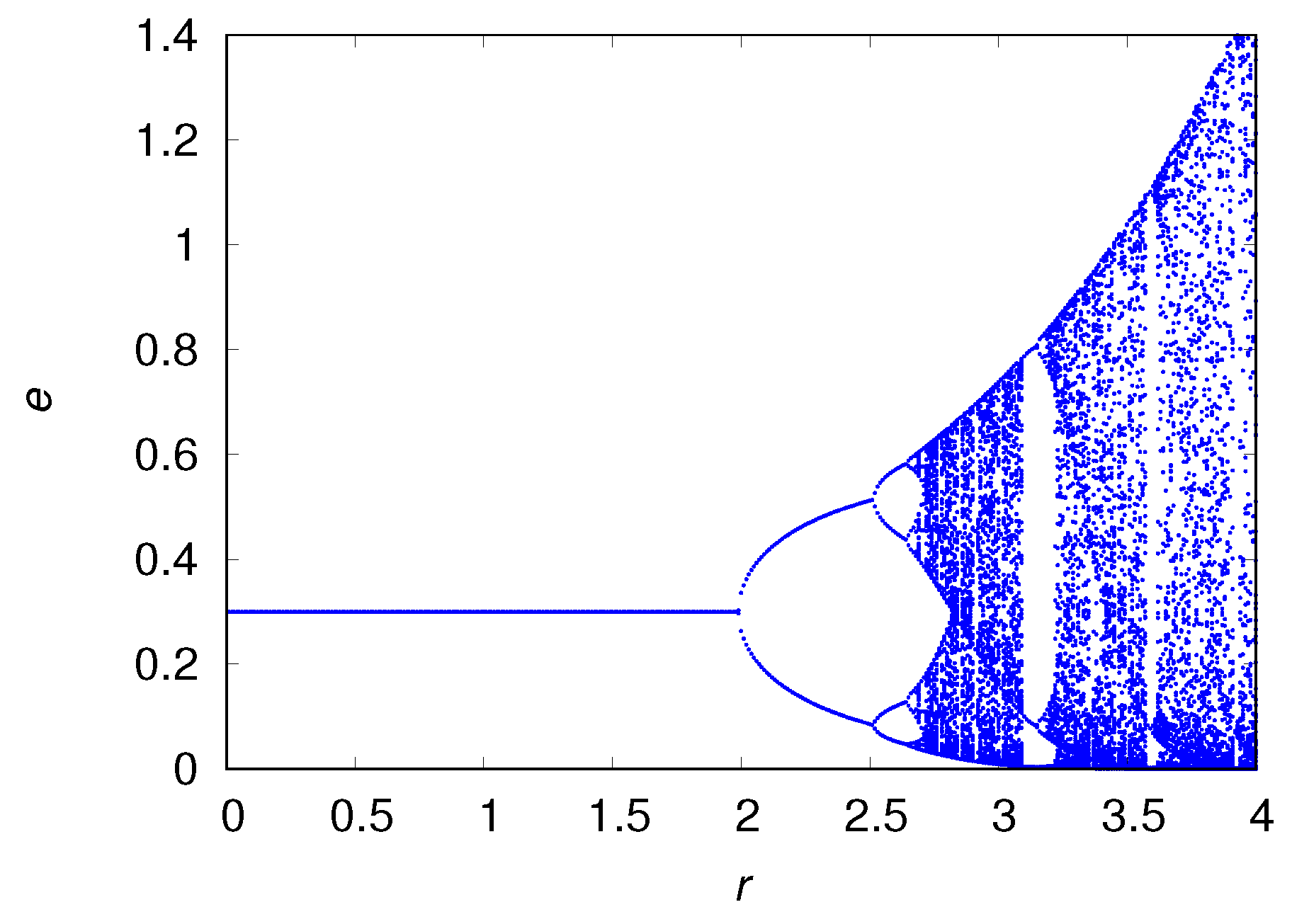
Figure 1 illustrates the dependence on the growth rate
r by showing the bifurcation diagram for the engineer density [
28]. The period-doubling bifurcation cascade is expected since the source of nonlinearity of the population dynamics is Ricker’s formula [
21].
Here our interest is on the nontrivial fixed-point solutions only, which are obtained by setting
,
and
in Equations (5)–(8). Assuming
we have
and
with
given by the solution of the transcendental equation
In the limit of small density, i.e.,
, this equation reduces to
and
, indicating that this fixed point is physical for
only. As expected,
increases with increasing
and
, and decreases with increasing
. Although Equation (9) does not depend on the growth rate
r, large values of this parameter lead to the instability of the fixed point
as illustrated in
Figure 1. Finally, the trivial fixed point
,
and
is stable for
. We refer the reader to Ref. [
12] for the detailed analysis of the local stability of the fixed points of the recursion Equations (5)–(8) .
3. The Coupled Map Lattice Version of the Gurney and Lawton Model
The space-independent recursion Equations (5)–(8) govern the local or single-patch population dynamics, where, as already pointed out, a patch is a complete ecosystem (e.g., an isle) with the three types of habitats and a population of engineers. Those equations describe the growing phase of the population of engineers. Here we introduce another phase: the dispersal phase, which we assume takes place before the growing stage. In particular, we consider a system of
N patches (e.g., an archipelago) and allow the engineers to circulate among neighboring patches, such that a fraction
of the population in patch
i is transferred to the
neighboring patches. Hence after the dispersal stage the population at patch
i is
where the sum is over the
nearest neighbors of patch
i. Note that since each term in the summation is divided by
, the fraction
of the population lost by patch
j is equally divided among the
neighboring patches. For simplicity, we assume that the total number of habitats
T is the same for all patches, so that the effect of dispersal on the density of engineers is given by
for patch
. After dispersal of the engineers, the growing stage takes place within each patch according to the equations
for
. Together with Equation (12), these equations form a coupled map lattice (see, e.g., [
29]) that describe the dynamics of the system of patches or metapopulation.
Since we are not interested on the formation of stationary spatial patterns, which for the Gurney and Lawton model appear only in the case the model parameters are such that the local dynamics (5)–(8) is chaotic [
12], the only patch arrangements we will consider in this paper are chains with an odd number of patches and reflective boundary conditions (i.e.,
and
). In addition, we will focus on a colonization or invasion scenario where at generation
only the central patch
of the chain is populated, whereas the other patches are composed entirely of virgin habitats (see, e.g., [
16]). In particular, we set
and
,
for all
.
In the next section we will study the time dependence of the mean density of engineers,
and the mean fraction of virgin habitats,
in the regime where the local dynamics is attracted to the nontrivial fixed point
, so we do not need to worry about accuracy issues caused by the chaotic amplification of numerical noise [
19].
4. Results
As our focus is on the time dependence of the global quantities and , the results of this section are obtained solely through the numerical iteration of the coupled map lattice Equations (12)–(15). In addition, since we expect that the time to reach the borders of the chain scales linearly with the chain size N, the results are presented in terms of the rescaled time .
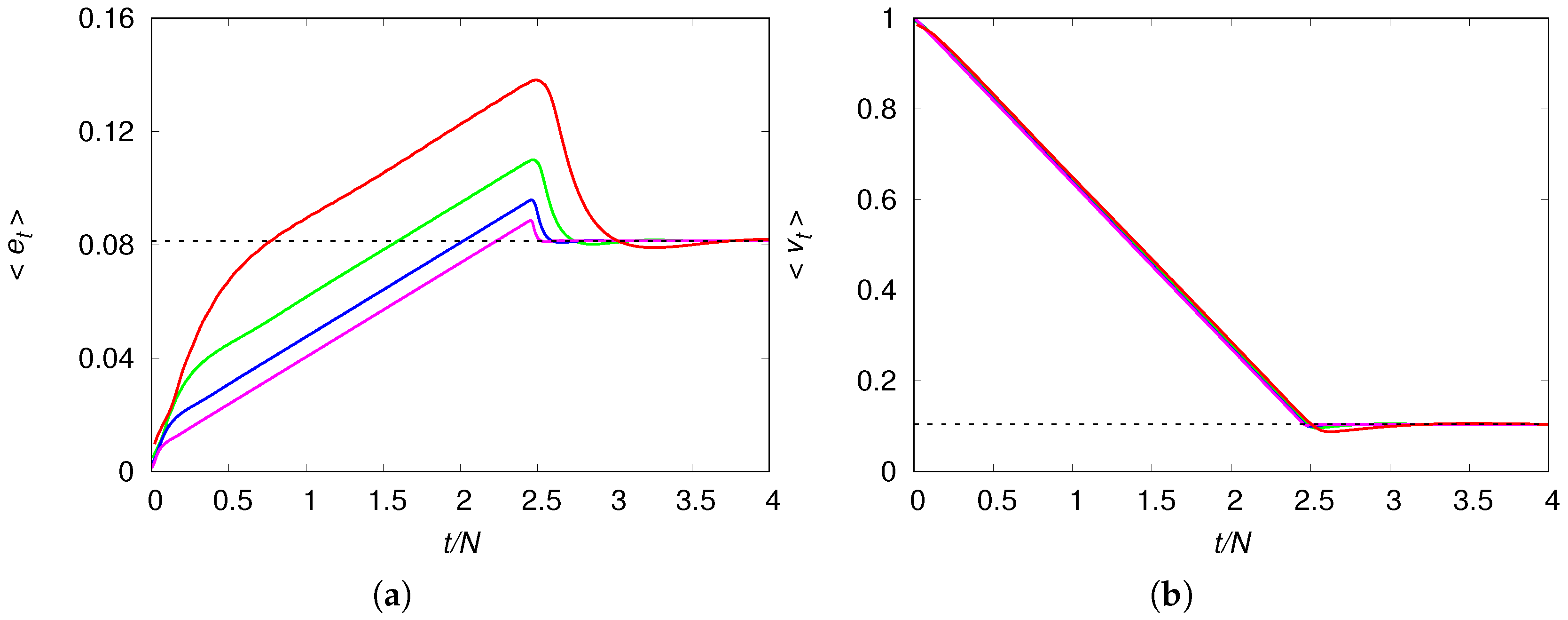
Figure 2 shows the evolution of the mean density of engineers and the mean fraction of virgin habitats for several chain sizes
N. It reveals the dramatic effect of the engineers’ mobility, which allow the population to reach densities well above those the environment could support in a situation of equilibrium. The initial increase of the mean density
reflects the expansion phase of the engineers, which is accompanied by the monotone decreasing of the unexplored patches, as expected. This expansion halts only when the engineers reach the borders of the chain and the end of the availability of unexplored virgin habitats results in a sharp drop on their density, which then quickly converges to the stationary value
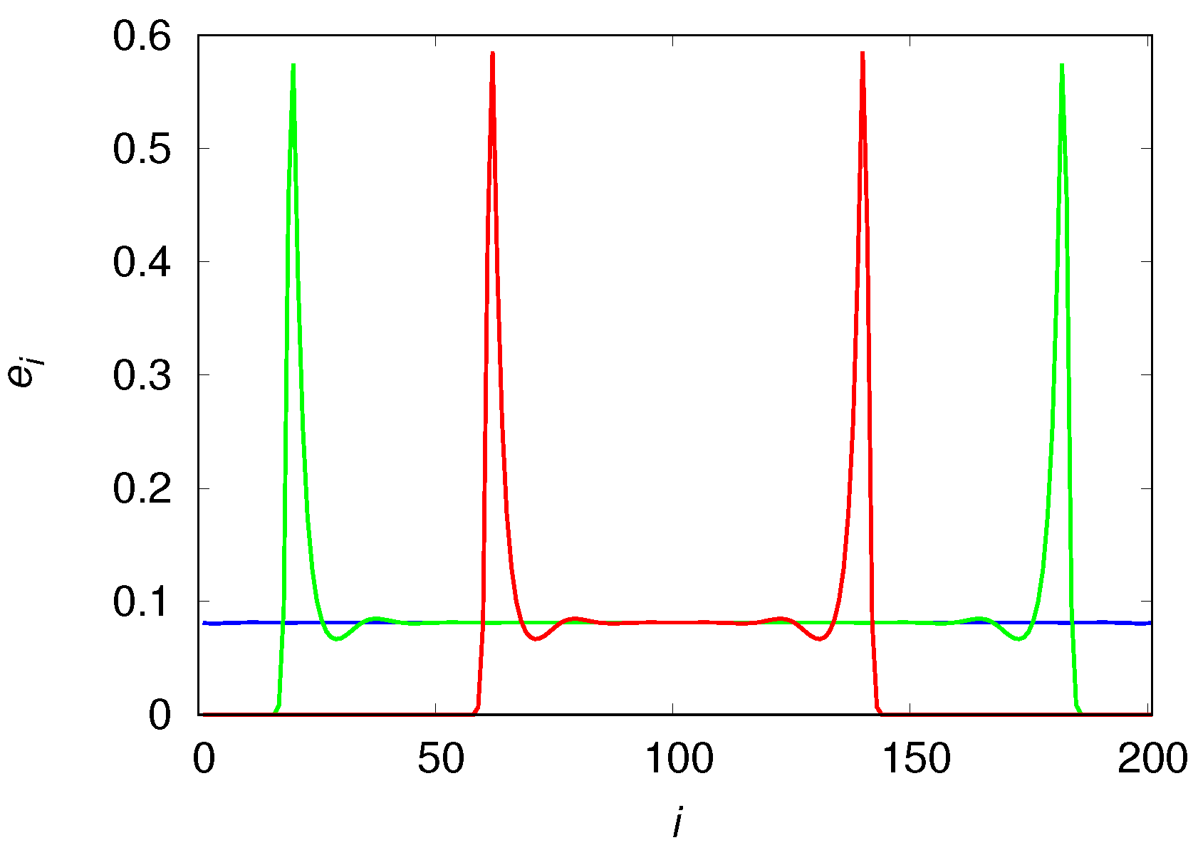
. This scenario is corroborated by
Figure 3 that shows the colonization wavefronts at three distinct times. The reason the size of the engineer density drop decreases with increasing
N (see panel (a) of
Figure 2) is simply because the contribution of the two high-density wavefronts is watered down by the equilibrium-density of the bulk of the chain. We note that the shape and height of the wavefronts are not affected by the chain size. The time evolution of the mean fraction of usable habitat is qualitatively similar to that shown in panel (a) for the density of engineers.
Figure 2 suggests a direct way to calculate the mean speed
of the colonization wavefronts, which is defined as the ratio between the distance from the center to the borders of the chain (i.e.,
) and the time
to reach those borders, i.e.,
In fact,
can be easily estimated by the time at which
is maximum. For instance, for all the chain sizes shown in
Figure 2, we find
, so that
. This means that it is necessary about five generations, on the average, for the wavefront peak to move between contiguous patches. Since the mean speed of the colonization wavefronts is very weakly influenced by the chain size, as illustrated in
Figure 2, henceforth we will consider chains of size
only.
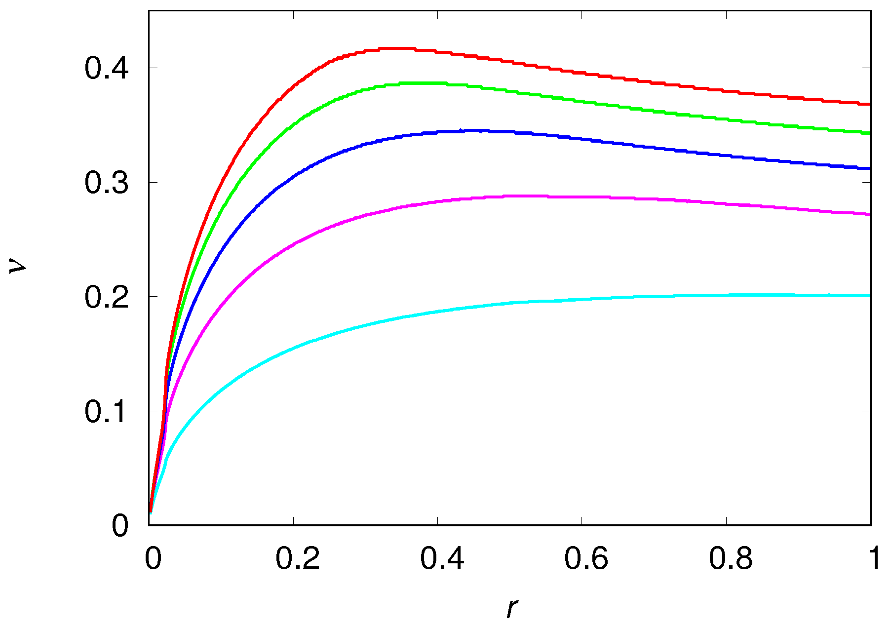
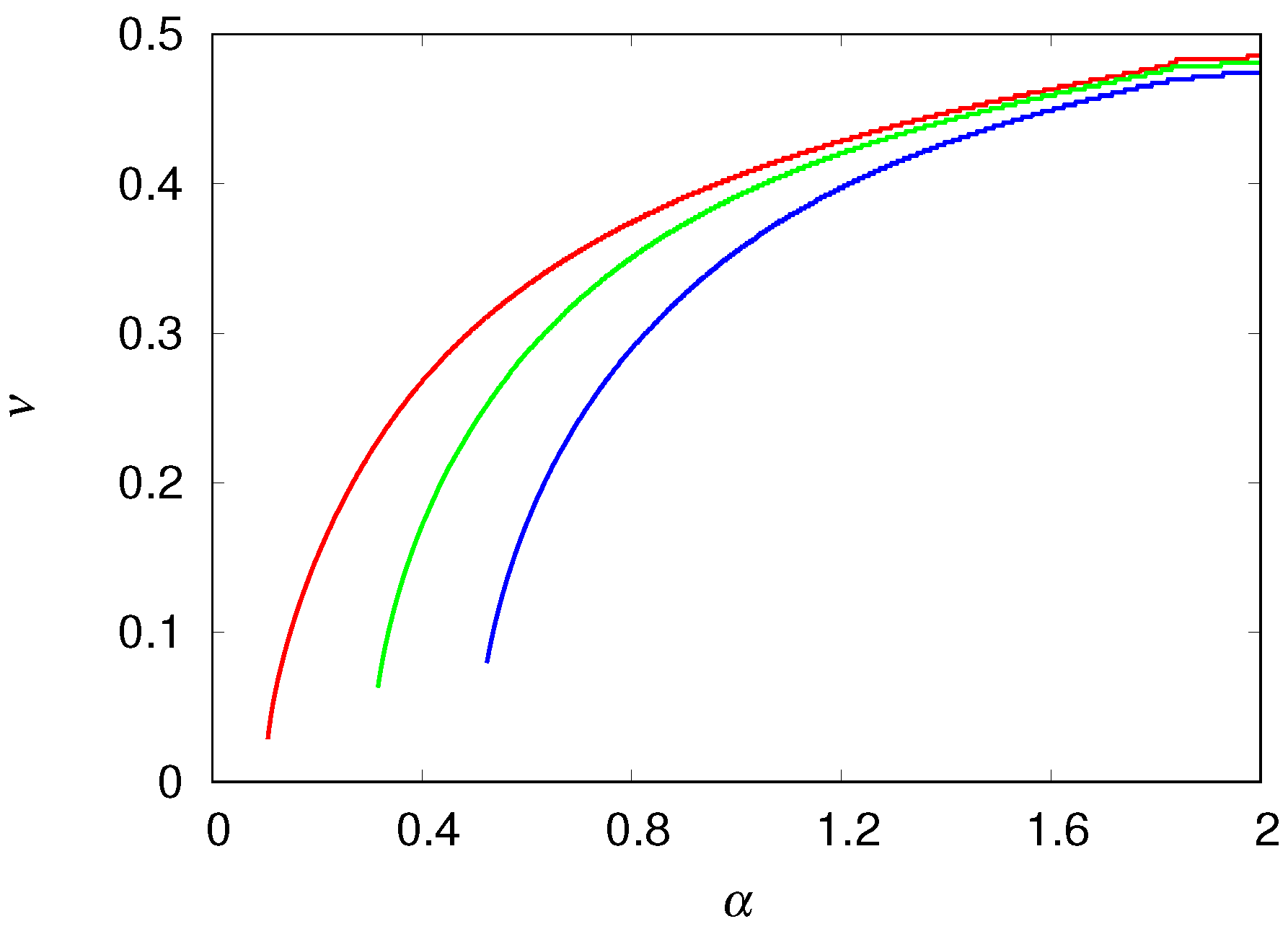
Figure 4 shows the dependence of the wavefront mean speed
on the growth rate
r and on the dispersal probability
. Although these two parameters have no effect whatsoever on the stationary solution
and
, they have a strong influence on the speed the population colonizes the unexplored patches. The speed
is a monotone increasing function of the dispersal probability
, as expected, and the rate of increase of
decreases with increasing
. The dependence of
on the growth rate
r is more interesting since it exhibits a non-monotone behavior, which is best seen in the figure for large values of the dispersal probability but that actually happens for all values of
. For instance, for
(cyan curve in
Figure 4) the maximum of
occurs for
at which we find
, whereas for
we find
. This variation is not perceptible in the scale of
Figure 4. Since only a fast growing population can guarantee a very large density at the borders of the expanding colony (see
Figure 3) and hence take advantage of the neighboring unexplored patches, one should expect a steep increase of
with increasing
r, despite the fact that
r plays no role in the equilibrium situation. In fact, this is what one observes in
Figure 4, provided that
r is not too large. The smooth decrease of
for large
r is probably due to the negative feedback of a large growth rate on the engineer population when the available fraction of useful habitats is not large enough. In fact, the maximum wavefront speed observed in the figure is a result of a fine tuning between the growth rate
r and the potential to create usable habitats
from the virgin patches. Interestingly, although the first engineers to reach the virgin patches are doomed to extinction because there are no usable habitats in those patches (see Equation (13)), they build the usable habitats (see Equation (15)) for the next wave of migrants.
We have verified that the mean speed
of the colonization wavefronts is not influenced by the recovery probability
of the degraded habitats, as expected. In fact, the capacity of recovery of the degraded habitats that are left far behind the invasion front is completely irrelevant for the survival and growth of the pioneers in the colonization front. The dependence of
on the productivity rate
and on the decay probability
is summarized in
Figure 5. The results are restricted to the region
where we can guarantee the existence of a viable equilibrium population of engineers, i.e.,
. The mean speed
increases monotonically with
since the efficiency of the transformation of virgin habitats into usable habitats is crucial for the survival of the second wave of migrants in the colonization front, as pointed out before. In the same line of reasoning, if the recently created usable habitats decay too rapidly, then the colonization front will be delayed as shown in
Figure 5. However, if the productivity
is large then the decay probability
has only a negligible retarding effect on the mean speed of the wavefront.
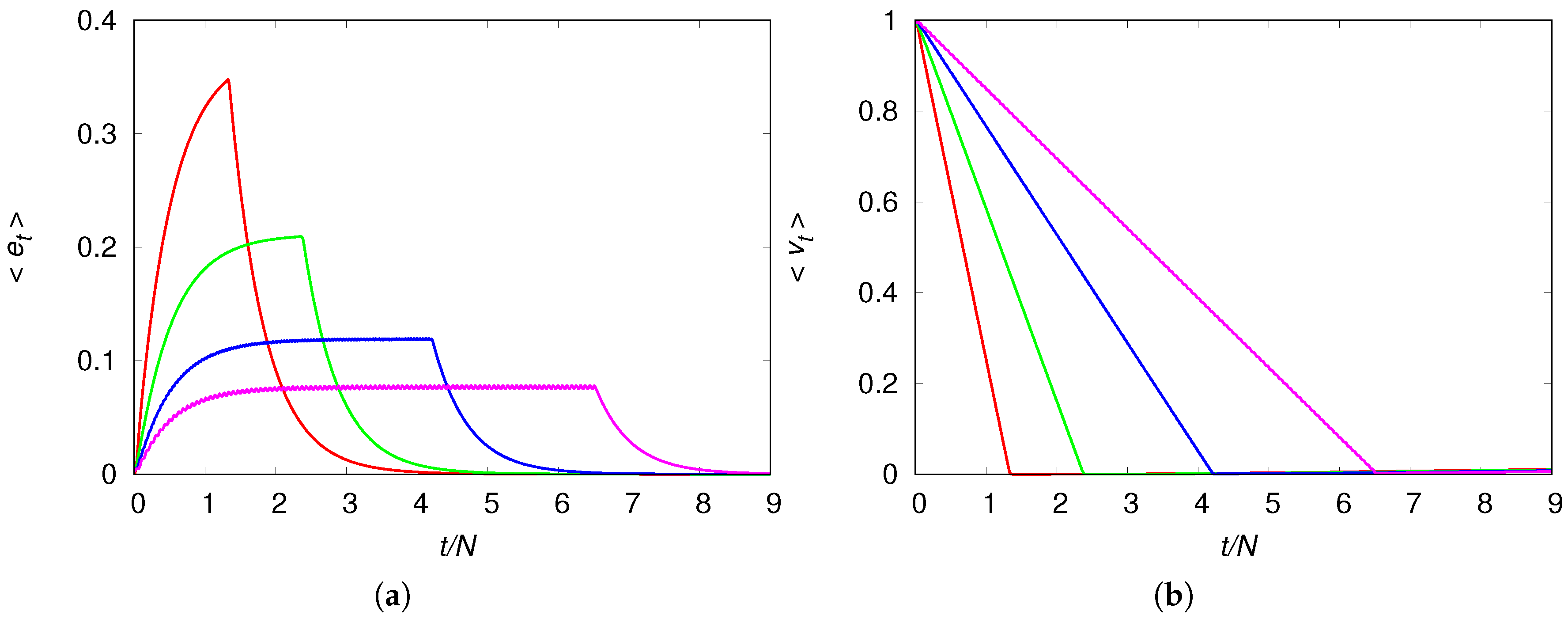
The collapse of the population, which happens when there are no more virgin patches to be explored, can be made more spectacular by setting the model parameters such that the equilibrium population density is very small, i.e.,
. One way to achieve this is by setting
(see Equation (10)), resulting in the global measures
and
displayed in
Figure 6. Let us consider first panel (b) of
Figure 6 that shows the linear decrease of the fraction of virgin habitats with time, which ends when the colonization fronts reach the borders of the chain at time
. At this moment we have
and from then on the fraction of virgin habitats begins to increase very slowly following the time scale set by the recovery probability
(this last stage is barely seen on the scale of the figure).
The time dependence of the density of engineers shown in panel (a) of
Figure 6 is more instructive. The population with the highest mobility uses up the environmental resources quickly and reaches very high densities before plunging towards the low equilibrium density, whereas the population with the lowest mobility can maintain an average density value for a long time before exhausting the resources. It is interesting that in this case the mean density of engineers exhibits a sort of metastable equilibrium, i.e.,
is practically constant for a period of time significantly longer than the initial increase (see the blue and magenta curves in panel (a) of
Figure 6), although the population is expanding through the unexplored patches.
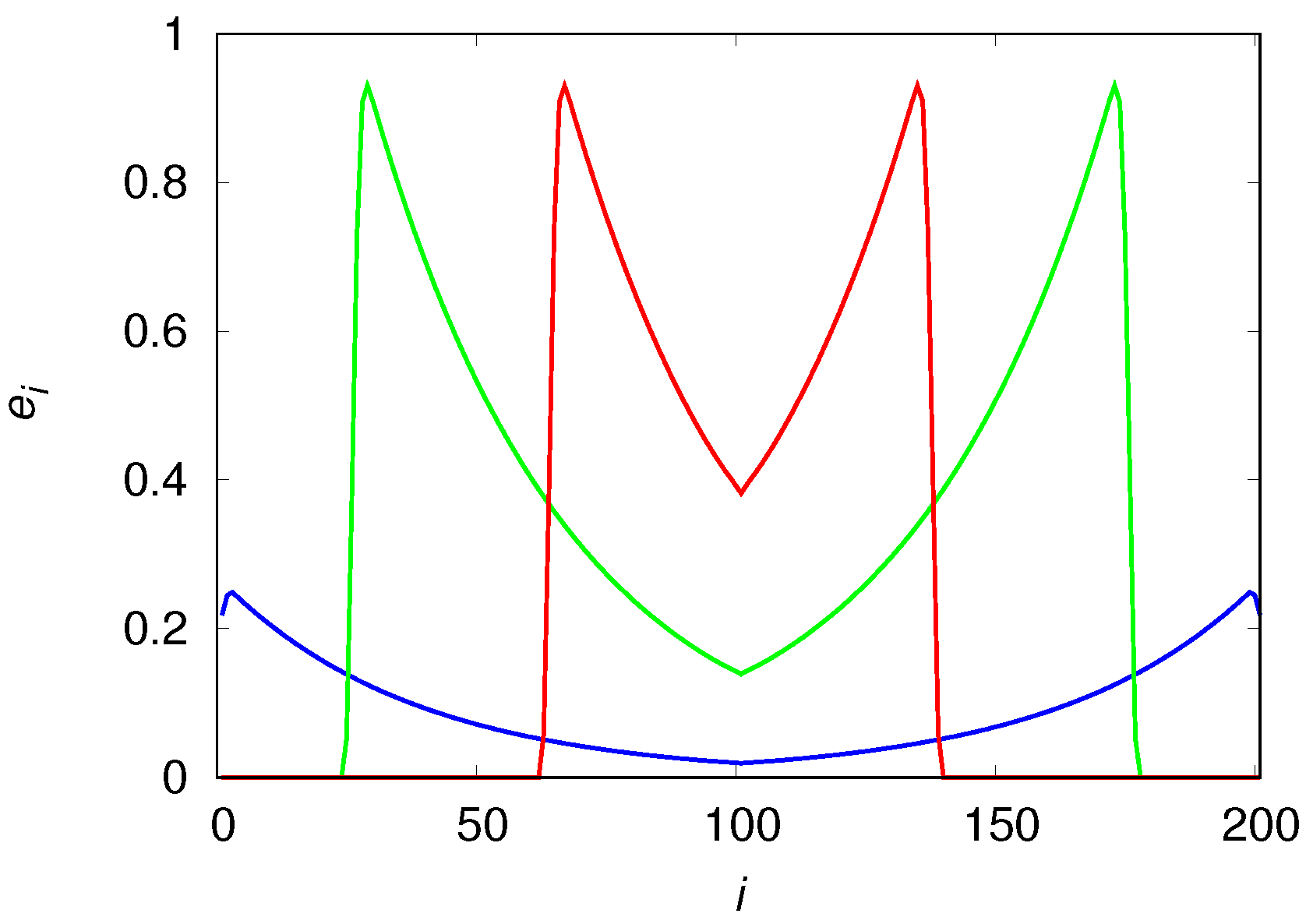
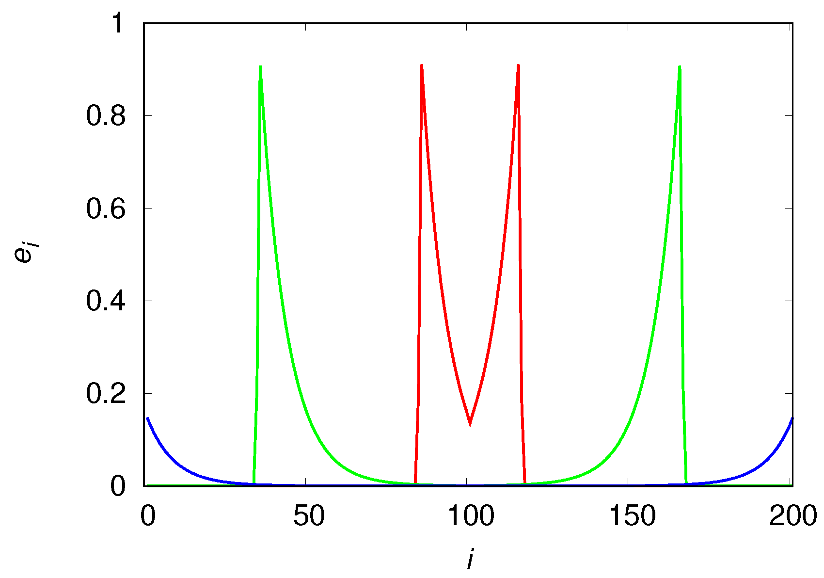
The qualitative differences of the population density in these mobility extremes are easily understood with the aid of
Figure 7 and
Figure 8 that show the population densities in each patch for
and
, respectively. In fact, the reason the high mobility population (see
Figure 7) attains such high densities before it collapses is simply that it reaches the borders before the usable habitats in the center of the chain can degrade appreciably. In the low mobility case (see
Figure 8), the center of the chain is practically desert when the colonization front is moving towards the borders. The metastable equilibrium mentioned before is simply a consequence of the invariance of the shape (or, more pointedly, of the area) of the wavefronts, as the colonization fronts are the only places where usable habitats are found (the spatial distribution of usable habitats is indistinguishable from that of the engineers). We note that the density near the borders is higher than near the center of the chain because the usable habitats at the borders were created much later than those in the center and so had less time to decay into the degraded class.
Finally, we note that in the case of inviable patches, i.e., in the regime where the nontrivial fixed point is unphysical and is stable, the colonization of the unexplored virgin patches fails and the engineers quickly go extinct. The reason is that the vast supply of unexplored patches is irrelevant if the production of usable habitats from them is not enough to balance the decay of the usable habitats into degraded habitats.
5. Discussion
The increase of the mean density of engineers
during the expansion phase of the colony is totally expected, of course, since as new patches are invaded by the engineers their overall density must increase. (We recall that in our scenario
varies from the arbitrarily set initial value
to the local equilibrium density
, where
N is the number of patches.) What is surprising is that the transient density reaches values much larger than the equilibrium density and plunges sharply when the colonization front hits the boundary of the available space (see, e.g.,
Figure 6). This phenomenon was observed en passant in Ref. [
12] for the regime of chaotic local dynamics, and was somewhat concealed by the difficulty of controlling the numerical accuracy of hundreds of chaotically oscillating coupled patches. Here we have offered a detailed analysis of the colonization process for the numerically more manageable dynamic regime where the sole attractors are fixed points.
We note that if we set the recovery probability
of the degraded habitats to a small value, then the equilibrium population density
will be small too (see Equation (
10)), and since the maximum mean density
does not depend on
, we get
, which implies a catastrophic reduction of the population density around time
. This is the reason we liken the sharp drop of the population density when the supply of unexplored resources is exhausted (see
Figure 2 and
Figure 6) to the collapse of ancient human societies that overexploited their environment [
7]. In that sense, we offer an alternative to the view that a population collapse involves the relatively quick decline of a population, which is established in the habitat considered. In our perspective, a collapse involves a population reaching physical or technological boundaries so that it can no longer sustain its over increased size.
In the context of the collapse of human societies, our population dynamics model produces two outcomes that are worth emphasizing. The first result is that for low mobility values the disaster comes without warning since the mean density
is practically constant before the collapse (see the blue and magenta curves in panel (a) of
Figure 6), and the width and height of the wavefront are constant before the colonization front hits the chain border (see
Figure 8). The disaster arrival is also silent for high mobility values since the mean density
and the width of the wavefront of colonization are still increasing when the collapse occurs (see red and green curves in panel (a) of
Figure 6 and
Figure 7). This accords with Diamond’s interpretation of the archaeological records of collapsed civilizations [
7]: “In fact, one of the main lessons to be learned from the collapses of the Maya, Anasazi, Easter Islanders, and those other past societies (as well as from the recent collapse of the Soviet Union) is that a society’s steep decline may begin only a decade or two after the society reaches its peak numbers, wealth, and power.”
The second consequence of our model is that overpopulation is a natural outcome of the nonlinear dynamics of the ecosystem engineer population expanding over unexplored habitats. A rough global measure of the overpopulation at time
t is given by the ratio
that equals one in the equilibrium situation. We note, however, that the local engineer density in the patches that are part of the colonization front are much higher than the overall mean density (see
Figure 3,
Figure 7 and
Figure 8). This is so because the second wave of migrants finds empty patches composed mostly of usable habitats (meaning a large carrying capacity) that resulted from the work of the extinct first wave of migrants on the original virgin habitats.
As a cautionary note on the adequacy of our approach to describe human populations, we should mention that the discrete-time map (
5)–(
8) assumes non-overlapping generations, which is clearly not the case for humans. Our justification to use this approach is a pragmatic one: discrete-time maps can easily be extended to describe space-dependent problems, resulting in coupled map lattices that can be thoroughly studied numerically. In addition, since here we consider the regime where the only attractors are stable fixed points, we do not expect any significant differences between the discrete and the continuous time approaches. In this line, we note that replacing Ricker model, Equation (
1), with a model that prevents large fluctuations on the population size, such as the Beverton-Holt model [
30], yields qualitatively the same results as those reported here, supporting thus our conjecture that our findings are robust to model details.
We find it quite remarkable that the model proposed by Gurney and Lawton to study the population dynamics of ecosystem engineers [
8], which seems to have been developed with an eye on the ecology of beavers [
3], could provide such interesting insights on the collapse dynamics of past human societies, without incorporating specific traits of those societies [
7]. For instance, one such a trait is existence of ruling elites that parasitize on the large mass of producers (commoners), using their workforce to produce luxury items and religious monuments [
10]. This feature could easily be incorporated in our model by requiring that only the commoners modify the virgin habitats and that the elite members use a disproportionally large amount of usable habitats. Another interesting possibility for future research is the introduction of multiplicative noise affecting the availability of virgin habitats aiming at modeling the effects of droughts and bonanzas in our model ecosystem [
31,
32]. Nonetheless, our results show that the collapse of an expanding population of ecosystem engineers seems to be a robust, unavoidable consequence of the nonlinear feedback between the population and environment variables, so a more detailed modeling of human societies will probably have little effect on our findings.
