On Some Extended Block Krylov Based Methods for Large Scale Nonsymmetric Stein Matrix Equations

Abstract

In the present paper, we consider the large scale Stein matrix equation with a low-rank constant term $AXB-X+E{F}^T=0$. These matrix equations appear in many applications in discrete-time control problems, filtering and image restoration and others. The proposed methods are based on projection onto the extended block Krylov subspace with a Galerkin approach (GA) or with the minimization of the norm of the residual. We give some results on the residual and error norms and report some numerical experiments.

1. Introduction

In this paper, we are interested in the numerical solution of large scale nonsymmetric Stein matrix equations of the form:

$$AXB-X+E{F}^T=0$$

(1)

where A and B are real, sparse and square matrices of size $n\times n$ and $s\times s,$ respectively, and E and F are matrices of size $n\times r$ and $s\times r$, respectively.

Stein matrix equations play an important role in many problems in control and filtering theory for discrete-time large-scale dynamical systems, in each step of Newton’s method for discrete-time algebraic Riccati equations, model reduction problems, image restoration techniques and other problems [1,2,3,4,5,6,7,8,9,10].

Direct methods for solving the matrix Equation (1), such as those proposed by Bartels–Stewart [11] and the Hessenberg–Schur [12] algorithms, are attractive if the matrices are of small size. For a general overview of numerical methods for solving the Stein matrix equation [1,2,13].

The Stein matrix Equation (1) can be formulated as an $ns\times ns$ large linear system using the Kronecker formulation:

$$(B^T\otimes A-I_s\otimes I_n)vec\left(X\right)=-vec\left(E{F}^T\right)$$

(2)

where $vec\left(X\right)$ is the vector obtained by stacking all the columns of the matrix X, $I_n$ is the n-by-n identity matrix, and the Kronecker product of two matrices A and B is defined by $A\otimes B=\left[a_{ij}B\right],$ where $A=\left[a_{ij}\right]$. This product satisfies the properties $(A\otimes B)(C\otimes D)=(AC\otimes BD)$, ${(A\otimes B)}^T=A^T\otimes B^T$ and $vec\left(AXB\right)=(B^T\otimes A)vec\left(X\right)$. Then, the matrix Equation (1) has a unique solution if and only if $\lambda \mu \ne 1$ for all $\lambda \in \sigma \left(A\right)$ and $\mu \in \sigma \left(B\right)$, where $\sigma \left(A\right)$ denotes the spectrum of the matrix A. Throughout the paper, we assume that this condition is satisfied. Moreover, if both A and B are Schur stable, i.e., $\sigma \left(A\right)$ and $\sigma \left(B\right)$ lie in the open unit disc, and then the solution of Equation (1) can be expressed as the following infinite matrix series:

$$X=\sum _{i=0}^{\infty }{A}^{i}E{F}^T{B}^i$$

To solve large linear matrix equations, several Krylov subspace projection methods have been proposed (see, e.g., [1,13,14,15,16,17,18,19,20,21,22,23,24] and the references therein). The main idea developed in these methods is to use a block Krylov subspace or an extended block Krylov subspace and then project the original large matrix equation onto these Krylov subspaces using a Galerkin condition or a minimization property of the obtained residual. Hence, we will be interested in these two procedures to get approximate solutions to the solution of the Stein matrix Equation (1). The rest of the paper is organized as follows. In the next section, we recall the extended block Krylov subspace and the extended block Arnoldi (EBA) algorithm with some properties. In Section 3, we will apply the Galerkin approach (GA) to Stein matrix equations by using the extended Krylov subspaces. In Section 4, we define the minimal residual (MR) method for Stein matrix equations by using the extended Krylov subspaces. We finally present some numerical experiments in Section 5.

2. The Extended Block Krylov Subspace Algorithm

In this section, we recall the EBA algorithm applied to $(A,V),$ where $V\in {\mathbb{R}}^{n\times r}$. The block Krylov subspace associated with $(A,V)$ is defined as:

$${\mathbb{K}}_m(A,V)=Range\left(\{V,AV,A^{2}V,\cdots ,A^{m-1}V\}\right)$$

The extended block Krylov subspace associated with the pair $(A,V)$ is given as:

$$\begin{array}{ccc}{\mathcal{K}}_m^e(A,V)\hfill & =\hfill & Range\{V,A^{-1}V,AV,A^{-2}V,A^{2}V,\cdots ,A^{m-1}V,A^{-m}V\})\hfill \\ & =\hfill & {\mathbb{K}}_m(A,V)+{\mathbb{K}}_m(A^{-1},A^{-1}V)\hfill \end{array}$$

The EBA Algorithm 1 is defined as follows [15,16,18,23]:

Algorithm 1. The Extended Block Arnoldi (EBA) Algorithm

(1) Inputs: A an $n\times n$ matrix, V an $n\times r$ matrix and m an integer (2) Compute the QR decomposition of $[V,A^{-1}V]$, i.e., $[V,A^{-1}V]=V_1\mathsf{\Lambda }$ (3) Set ${\mathbb{V}}_0=\left[\right]$ (4) for $j=1,2,\dots ,m$ (a) Set $V_j^{\left(1\right)}$: first r columns of $V_j$; $V_j^{\left(2\right)}$: second r columns of $V_j$ (b) ${\mathbb{V}}_j=\left[{\mathbb{V}}_{j-1},V_j\right]$; ${\widehat{V}}_{j+1}=\left[A{V}_j^{\left(1\right)},A^{-1}{V}_j^{\left(2\right)}\right]$ (c) Orthogonalize ${\widehat{V}}_{j+1}$ w.r. to ${\mathbb{V}}_j$ to get $V_{j+1}$, i.e. ∗ for $i=1,2,\dots ,j$ ∗ ${\displaystyle H_{i,j}=V_i^T{\widehat{V}}_{j+1};}$ ∗ ${\displaystyle {\widehat{V}}_{j+1}={\widehat{V}}_{j+1}-V_i{H}_{i,j}}$ ∗ End for (d) Compute the $QR$ decomposition of ${\widehat{V}}_{j+1}$, i.e., ${\widehat{V}}_{j+1}=V_{j+1}{H}_{j+1,j}$ (5) End For

This algorithm allows us to construct an orthonormal matrix ${\mathbb{V}}_m=\left[V_1,V_2,\dots ,V_m\right]$ that is a basis of the block extended Krylov subspace ${\mathcal{K}}_m^e(A,V)$. The restriction of the matrix A to the block extended Krylov subspace ${\mathcal{K}}_m^e(A,V)$ is given by ${\mathbb{T}}_m={\mathbb{V}}_m^{T}A{\mathbb{V}}_m$.

Let ${\overline{\mathbb{T}}}_m={\mathbb{V}}_{m+1}^{T}A{\mathbb{V}}_m$. Then, we have the following relations [25]:

$$\begin{array}{lll}A{\mathbb{V}}_m& =& {\mathbb{V}}_{m+1}{\overline{\mathbb{T}}}_m\\ & =& {\mathbb{V}}_m{\mathbb{T}}_m+V_{m+1}{T}_{m+1,m}{\mathbb{E}}_m^T\end{array}$$

where ${\mathbb{E}}_m={[0_{2r\times 2(m-1)r},I_{2r}]}^T$ is the matrix of the last $2r$ columns of the identity matrix $I_{2mr}$ [23,25]. In the next section, we will define the GA for solving Stein matrix equations.

3. Galerkin-Based Methods

In this section, we will apply the Galerkin projection method to obtain low-rank approximate solutions of the nonsymmetric Stein matrix Equation (1). This approach has been applied for Lyapunov, Sylvester or Riccati matrix equations [1,14,15,19,20,21,23,25,26].

3.1. The Case: Both A and B Are Large Matrices

We consider here a nonsymmetric Stein matrix equation, where A and B are large and sparse matrices with $r\ll n$ and $r\ll s$. We project the initial problem by using the extended block Krylov subspaces ${\mathcal{K}}_m^e(A,E)$ and ${\mathcal{K}}_m^e(B^T,F)$ associated with the pairs $(A,E)$ and $(B^T,F)$, respectively, and get orthonormal bases $\{V_1,V_2,\dots ,V_m\}$ and $\{W_1,W_2,\dots ,W_m\}$. We then consider approximate solutions of the Stein matrix Equation (1) that have the low-rank form:

$$X_m^{GA}={\mathbb{V}}_m{Y}_m^{GA}{\mathbb{W}}_m^T$$

(3)

where ${\mathbb{V}}_m=\left[V_1,V_2,\dots ,V_m\right]$ and ${\mathbb{W}}_m=\left[W_1,W_2,\dots ,W_m\right]$.

The matrix $Y_m^{GA}$ is determined from the following Galerkin orthogonality condition:

$${\mathbb{V}}_m^T{\mathcal{R}}_m^{GA}{\mathbb{W}}_m={\mathbb{V}}_m^T(A{X}_m^{GA}B-X_m^{GA}+E{F}^T){\mathbb{W}}_m=0$$

(4)

Now, replacing $X_m^{GA}={\mathbb{V}}_m{Y}_m^{GA}{\mathbb{W}}_m^T$ in Equation (4), we obtain the reduced Stein matrix equation:

$${\mathbb{T}}_A{Y}_m^{GA}{\left({\mathbb{T}}_B\right)}^T-Y_m^{GA}+\tilde{E}{\tilde{F}}^T=0$$

(5)

where $\tilde{E}={\mathbb{V}}_m^{T}E$, $\tilde{F}={\mathbb{W}}_m^{T}F$, ${\mathbb{T}}_A={\mathbb{V}}_m^{T}A{\mathbb{V}}_m,\mathrm{and}{\mathbb{T}}_B={\mathbb{W}}_m^T{B}^T{\mathbb{W}}_m.$

Assuming that ${\lambda }_i\left({\mathbb{T}}_A\right){\lambda }_j\left({\mathbb{T}}_B\right)\ne 1$ for any $i=1,2,\dots ,2mr$ and $j=1,2,\dots ,2mr$, the solution $Y_m$ of the low-order Stein Equation (5) can be obtained by a direct method such as those described in [11]. The following result on the norm of the residual ${\mathcal{R}}_m$ allows us to stop the iterations without having to compute the approximation $X_m^{GA}$.

Theorem 1.

Let $X_m^{GA}$ be the approximation obtained at step m by the EBA algorithm. Then, the Frobenius norm of the residual ${\mathcal{R}}_m^G$ associated to the approximation $X_m^{GA}$ is given by:

$$\parallel {\mathcal{R}}_m^G{\parallel }_F=\sqrt{{\alpha }_m^2+{\beta }_m^2+{\gamma }_m^2}$$

(6)

where ${\alpha }_m={∥{\mathbb{T}}_m^A{Y}_m{\mathbb{E}}_m{\left(T_{m+1,m}^B\right)}^T∥}_F,{\beta }_m={∥T_{m+1,m}^A{\mathbb{E}}_m^T{\left({\mathbb{T}}_m^B\right)}^T∥}_F,$ and:

$${\gamma }_m={∥T_{m+1,m}^A{\mathbb{E}}_m^T{Y}_m{\mathbb{E}}_m{\left(T_{m+1,m}^B\right)}^T∥}_F$$

Proof. 

The proof is similar to the one given at proposition 6 in [17].  ☐

In the following result, we give an upper bound for the norm of the error $X-X_m^{GA}$.

Theorem 2.

Assume that ${\parallel A\parallel }_2<1$ and ${\parallel B\parallel }_2<1$, and let $Y_m^{GA}$ be the exact solution of projected Stein matrix Equation (5) and $X_m^{GA}$ be the approximate solution given by running m steps of the EBA algorithm. Then:

$$\parallel X-X_m^{GA}{\parallel }_2\le \frac{{\parallel A\parallel }_2\parallel T_{m+1,m}^B{\parallel }_2+{\parallel B\parallel }_2\parallel T_{m+1,m}^A{\parallel }_2+\parallel T_{m+1,m}^A{\parallel }_2{\parallel T_{m+1,m}^B\parallel }_2}{1-{\parallel A\parallel }_2{\parallel B\parallel }_2}{\parallel Y_m\parallel }_2$$

(7)

Proof. 

The proof is similar to the one given at Theorem 2 in [27].  ☐

The approximate solution $X_m^{GA}$ can be given as a product of two matrices of low rank. Consider the singular value decomposition of the $2mr\times 2mr$ matrix:

$$Y_m^{GA}={\tilde{Y}}_1\Sigma {\tilde{Y}}_2^T$$

where $\Sigma$ is the diagonal matrix of the singular values of $Y_m^{MR}$ sorted in decreasing order. Let $Y_{1,l}$ and $Y_{2,l}$ be the $2mr\times l$ matrices of the first l columns of ${\tilde{Y}}_1$ and ${\tilde{Y}}_2,$ respectively, corresponding to the l singular values of magnitude greater than some tolerance. We obtain the truncated singular value decomposition:

$$Y_m^{GA}\approx U_{1,l}{\Sigma }_l{U_{2,l}}^T$$

where ${\Sigma }_l=\mathrm{diag}[{\sigma }_1,\dots ,{\sigma }_l]$. Setting $Z_{1,m}={\mathbb{V}}_m{U}_{1,l}{\Sigma }_l^{1/2}$, and $Z_{2,m}={\mathbb{W}}_m{U}_{2,l}{\Sigma }_l^{1/2},$ it follows that:

$$X_m^{GA}\approx Z_{1,m}{Z}_{2,m}^T$$

(8)

This is very important for large problems when one doesn’t need to compute and store the approximation $X_m$ at each iteration.

The GA is given in Algorithm 2:

Algorithm 2. Galerkin Approach (GA) for the Stein Matrix Equations

(1) Inputs: A an $n\times n$ matrix, B an $s\times s$ matrix, E an $n\times r$ matrix and F an $s\times r$ matrix. (2) Choose a tolerance $tol>0$, a maximum number of $itermax$ iterations. (3) For $m=1,2,3,\dots ,itermax$ (4) Compute ${\mathbb{V}}_m,{\mathbb{T}}_m^A$, by Algorithm 1 applied to $(A,E).$ (5) Compute ${\mathbb{W}}_m,{\mathbb{T}}_m^B$, by Algorithm 1 applied to $(B^T,F).$ (6) Solve the low order Stein Equation (5) and compute $\parallel {\mathcal{R}}_m{\parallel }_F$ given by Equation (6) (7) if $\parallel {\mathcal{R}}_m{\parallel }_F\le tol$, stop, (8) Using Equation (8), the approximate solution $X_m^{GA}$ is given by $X_m^{GA}\approx Z_{1,m}{Z}_{2,m}^T$.

In the next section, we consider the case where the matrix A is large while B has a moderate or a small size.

3.2. The Case: A Large and B Small

In this section, we consider the Stein matrix equation:

$$AXB-X+E=0$$

(9)

where E is a matrix of size $n\times s$ with $s<<n$.

In this case, we will consider approximations of the exact solution X as:

$$X_m={\mathbb{V}}_m{Y}_m$$

where ${\mathbb{V}}_m$ is the orthonormal basis obtained by applying the extended block Krylov subspace ${\mathcal{K}}_m^e(A,E)$. The orthogonality Galerkin condition gives:

$${\mathbb{V}}_m^T{\mathcal{R}}_m=0$$

(10)

where ${\mathcal{R}}_m$ is the m-th residual given by ${\mathcal{R}}_m=A{X}_{m}B-X_m+E$. Therefore, we obtain the projected Stein matrix equation:

$${\mathbb{T}}_A{Y}_m^{GA}B-Y_m^{GA}+\tilde{E}=0$$

(11)

where ${\mathbb{T}}_A={\mathbb{V}}_m^{T}A{\mathbb{V}}_m$ and $\tilde{E}={\mathbb{V}}_m^{T}E$.

The next result gives a useful expression of the norm of the residual.

Theorem 3.

Let $Y_m^{GA}$ the exact solution of the reduced Stein matrix Equation (11) and let $X_m^{GA}={\mathbb{V}}_m{Y}_m^{GA}$ be the approximate solution of Equation (9) with ${\mathcal{R}}_m=\mathcal{R}\left(X_m^{GA}\right)$ the corresponding residual. Then:

$$\parallel {\mathcal{R}}_m{\parallel }_F={∥T_{m+1,m}^A{\mathbb{E}}_m^T{Y}_m^{GA}B∥}_F$$

(12)

Proof. 

The residual is given by ${\mathcal{R}}_m=A{X}_m^{GA}B-X_m^{GA}+E$. Since E is belonging to ${\mathcal{K}}_m^e(A,E)$, then ${\mathbb{V}}_m{\mathbb{V}}_m^{T}E=E$. Using the relation $A{\mathbb{V}}_m={\mathbb{V}}_{m+1}{\overline{\mathbb{T}}}_m^A$, we have:

$$\begin{array}{ccc}\hfill \parallel {\mathcal{R}}_m{\parallel }_F& =& {\displaystyle {∥A{\mathbb{V}}_m{Y}_m^{GA}B-{\mathbb{V}}_m{Y}_m^{GA}+E∥}_F}\hfill \\ & =& {\displaystyle {∥{\mathbb{V}}_{m+1}{\overline{\mathbb{T}}}_m^A{Y}_m^{GA}B-{\mathbb{V}}_m{Y}_m^{GA}+{\mathbb{V}}_m{\mathbb{V}}_m^{T}E∥}_F}\hfill \\ & =& {\displaystyle {∥{\mathbb{V}}_{m+1}{\overline{\mathbb{T}}}_m^A{Y}_m^{GA}B-{\mathbb{V}}_{m+1}\left(\begin{array}{c}I\\ 0\end{array}\right)Y_m^{GA}+{\mathbb{V}}_{m+1}\left(\begin{array}{c}I\\ 0\end{array}\right)\tilde{E}∥}_F}\hfill \\ & =& {\displaystyle {∥{\mathbb{V}}_{m+1}\left[{\overline{\mathbb{T}}}_m^A{Y}_m^{GA}B-\left(\begin{array}{c}I\\ 0\end{array}\right)Y_m^{GA}+\left(\begin{array}{c}\tilde{E}\\ 0\end{array}\right)\right]∥}_F}\hfill \end{array}$$

As the matrix ${\mathbb{V}}_{m+1}$ is orthogonal and ${\overline{\mathbb{T}}}_m^A=\left[\begin{array}{c}{\mathbb{T}}_m^A\\ T_{m+1,m}^A{\mathbb{E}}_m^T\end{array}\right]$, we have:

$$\begin{array}{ccc}\hfill \parallel {\mathcal{R}}_m{\parallel }_F& =& {\displaystyle {∥\left[\left[\begin{array}{c}{\mathbb{T}}_m^A\\ T_{m+1,m}^A{\mathbb{E}}_m^T\end{array}\right]Y_m^{GA}B-\left(\begin{array}{c}{Y}_m^{GA}\\ 0\end{array}\right)+\left(\begin{array}{c}\tilde{E}\\ 0\end{array}\right)\right]∥}_F}\hfill \\ & =& {\displaystyle {∥\left[\left(\begin{array}{c}{\mathbb{T}}_m^A{Y}_m^{GA}B-Y_m^{GA}+\tilde{E}\\ T_{m+1,m}^A{\mathbb{E}}_m^T{Y}_m^{GA}B\end{array}\right)\right]∥}_F}\hfill \end{array}$$

Therefore:

$$\parallel {\mathcal{R}}_m{\parallel }_F={∥T_{m+1,m}^A{\mathbb{E}}_m^T{Y}_m^{GA}B∥}_F$$

☐

This result is very important because it allows us to calculate the Frobenius norm of ${\mathcal{R}}_m\left(X_m^{GA}\right)$ without having to compute the approximate solution.

Next, we give a result showing that the error $X-X_m$ is an exact solution of a perturbed Stein matrix equation.

Theorem 4.

Let $X_m$ be the approximate solution of Equation (9) obtained after m iterations of the EBA algorithm. Then:

$$(A-F_m)X_{m}B-X_m=E$$

(13)

where $F_m=V_{m+1}{T}_{m+1,m}^A{V}_m^T.$

Proof. 

Multiplying the Equation (11) from the left by ${\mathbb{V}}_m$, we obtain:

$$[A{\mathbb{V}}_m-V_{m+1}{T}_{m+1,m}^A{\mathbb{E}}_m^T]Y_{m}B-{\mathbb{V}}_m{Y}_m={\mathbb{V}}_m\tilde{E}$$

(14)

As ${\mathbb{V}}_m\tilde{E}=E$, we get:

$$(A-F_m)X_{m}B-X_m=E$$

(15)

where:

$$F_m=V_{m+1}{T}_{m+1,m}^A{V}_m^T$$

☐

We can now state the following result, which gives an upper bound for the norm of the error.

Theorem 5.

If ${\parallel A\parallel }_2<1$ and ${\parallel B\parallel }_2<1$, then we have:

$$\parallel X-X_m{\parallel }_2\le \frac{\parallel T_{m+1,m}^A{\mathbb{E}}_m{Y}_{m}B{\parallel }_2}{1-{\parallel A\parallel }_2{\parallel B\parallel }_2}$$

(16)

Proof. 

By subtracting Equation (13) from Equation (9), we get:

$$A(X-X_m)B-(X-X_m)=-F_m{X}_{m}B$$

(17)

The error $X_m-X$ is the solution of the Stein matrix Equation (17) and can be expressed as:

$$X_m-X=\sum _{i=0}^{+\infty }{A}^i\left[F_m{X}_{m}B\right]B^i$$

(18)

$$\begin{array}{ccc}\hfill \parallel X_m{-X\parallel }_2& \le & \sum _{i=0}^{+\infty }\parallel A^i{\parallel }_2\parallel F_m{X}_m{B\parallel }_2{\parallel B^i\parallel }_2\hfill \end{array}$$

(19)

$$\begin{array}{cc}\le & \parallel F_m{X}_m{B\parallel }_2\sum _{i=0}^{+\infty }{\left({\parallel A\parallel }_2{\parallel B\parallel }_2\right)}^i\hfill \end{array}$$

(20)

$$\begin{array}{cc}\le & \frac{\parallel F_m{X}_m{B\parallel }_2}{1-{\parallel A\parallel }_2{\parallel B\parallel }_2}\hfill \end{array}$$

(21)

$$\begin{array}{cc}\le & \frac{\parallel T_{m+1,m}^A{E}_m{Y}_m{B\parallel }_2}{1-{\parallel A\parallel }_2{\parallel B\parallel }_2}\hfill \end{array}$$

(22)

☐

In the next section, we present projection methods based on extended block Krylov subspaces and MR property.

4. Minimal Residual Method for Large Scale Stein Matrix Equations

In this section, we present a MR method for solving large scale Stein matrix equations. A MR method for solving large scale Lyapunov matrix equation is given in [22].

4.1. The Case: Both A and B Are Large

Instead of using a Galerkin condition as we explained in the preceding section, we consider here approximate solutions $X_m^{MR}={\mathbb{V}}_m{Y}_m^{MR}{\mathbb{W}}_m^T$ satisfying the following minimization property:

$$X^{MR}=arg\underset{X_m={\mathbb{V}}_m{Y}_m{\mathbb{W}}_m^T}{min}{∥A{X}_{m}B-X_m+E{F}^T∥}_F$$

(23)

We have the following result.

Theorem 6.

The solution $X_m^{MR}$ of the the minimization problem:

$${\displaystyle X_m^{MR}=arg\underset{X_m={\mathbb{V}}_m{Y}_m{\mathbb{W}}_m^T}{min}{∥A{X}_{m}B-X_m+E{F}^T∥}_F}$$

is given by:

$$X_m^{MR}={\mathbb{V}}_m{Y}_m^{MR}{\mathbb{W}}_m^T$$

where $Y_m^{MR}$ solves the following low dimentional minimization problem:

$$Y_m^{MR}=argmin{∥{\overline{\mathbb{T}}}_m^A{Y}_m{\left({\overline{\mathbb{T}}}_m^B\right)}^T-\left(\begin{array}{c}I\\ 0\end{array}\right)Y_m\left(\begin{array}{cc}I& 0\end{array}\right)+\left(\begin{array}{cc}{R}_E{R}_F^T& 0\\ 0& 0\end{array}\right)∥}_F$$

(24)

with $E=V_1{R}_E$ and $F=W_1{R}_F$, the $QR$ factorization of E and F, respectively.

Proof. 

We have:

$$\begin{array}{c}{\displaystyle \underset{X={\mathbb{V}}_m{Y}_m{\mathbb{W}}_m^T}{min}{∥AXB-X+E{F}^T∥}_F}\hfill \\ {\displaystyle =\underset{Y_m}{min}{∥A{\mathbb{V}}_m{Y}_m{\mathbb{W}}_m^{T}B-{\mathbb{V}}_m{Y}_m{\mathbb{W}}_m^T-V_1{R}_E{R}_F^T{W}_1^T∥}_F}\hfill \\ {\displaystyle =\underset{Y_m}{min}{∥{\mathbb{V}}_{m+1}\left[{\overline{\mathbb{T}}}_m^A{Y}_m{\left({\overline{\mathbb{T}}}_m^B\right)}^T-\left(\begin{array}{c}I\\ 0\end{array}\right)Y_m\left(\begin{array}{cc}I& 0\end{array}\right)+\left(\begin{array}{cc}{R}_E{R}_F^T& 0\\ 0& 0\end{array}\right)\right]{\mathbb{W}}_{m+1}^T∥}_F}\hfill \\ {\displaystyle =\underset{Y_m}{min}{∥\left[{\overline{\mathbb{T}}}_m^A{Y}_m{\left({\overline{\mathbb{T}}}_m^B\right)}^T-\left(\begin{array}{c}I\\ 0\end{array}\right)Y_m\left(\begin{array}{cc}I& 0\end{array}\right)+\left(\begin{array}{cc}{R}_E{R}_F^T& 0\\ 0& 0\end{array}\right)\right]∥}_F}\hfill \end{array}$$

☐

One advantage of using the minimization approach is the fact that the projected problem (24) always has a solution that is not the case when one uses a GA.

The main problem is now how to solve the reduced order minimization problem (24). One possibility is the use of the preconditioned global conjugate gradient (PGCG) method.

4.2. The Preconditioned Global CG Method for Solving the Reduced Minimization Problem

In this section, we adopt the preconditioned conjugate gradient method (PCG) [28,29] to solve the reduced minimization problem (24). The normal equation associated with (24) is given by:

$${\mathcal{L}}_m^{\ast }\left({\mathcal{L}}_m\left(Y\right)\right)={\mathcal{L}}_m^{\ast }\left(\mathcal{C}\right)$$

(25)

where:

$${\mathcal{L}}_m\left(Y\right)={\overline{\mathbb{T}}}_m^{A}Y{\left({\overline{\mathbb{T}}}_m^B\right)}^T-\left(\begin{array}{c}I\\ 0\end{array}\right)Y\left(\begin{array}{cc}I& 0\end{array}\right)$$

Notice that ${\mathcal{L}}_m^{\ast }$ is the adjoint of the linear operator ${\mathcal{L}}_m$ with respect to the Frobenius inner product is given by:

$${\mathcal{L}}_m^{\ast }\left(Z\right)={\left({\overline{\mathbb{T}}}_m^A\right)}^{T}Z{\overline{\mathbb{T}}}_m^B-\left(\begin{array}{cc}I& 0\end{array}\right)Z\left(\begin{array}{c}I\\ 0\end{array}\right)$$

and:

$$\mathcal{C}=\left(\begin{array}{cc}{R}_E{R}_F^T& 0\\ 0& 0\end{array}\right)$$

We can decompose the matrices ${\overline{\mathbb{T}}}_m^A$ and ${\overline{\mathbb{T}}}_m^B$ as follows:

$${\overline{\mathbb{T}}}_m^A=\left(\begin{array}{c}{\mathbb{T}}_m^A\\ h_m^A\end{array}\right)\mathrm{and}{\overline{\mathbb{T}}}_m^B=\left(\begin{array}{c}{\mathbb{T}}_m^B\\ h_m^B\end{array}\right)$$

where $h_m^A$ and $h_m^B$ represent the last $2r$ rows of the matrices ${\overline{\mathbb{T}}}_m^A$ and ${\overline{\mathbb{T}}}_m^B$, respectively. Therefore, the normal Equation (25) can be written as:

$${{\overline{\mathbb{T}}}_m^A}^T{\overline{\mathbb{T}}}_m^{A}Y{{\overline{\mathbb{T}}}_m^B}^T{\overline{\mathbb{T}}}_m^B+Y-{{\mathbb{T}}_m^A}^{T}Y{\mathbb{T}}_m^B-{\mathbb{T}}_m^{A}Y{\left({\mathbb{T}}_m^B\right)}^T-{\mathcal{L}}_m^{\ast }\left(\mathcal{C}\right)=0$$

(26)

Considering the singular value decomposition (SVD) of the matrices ${\overline{\mathbb{T}}}_m^A$ and ${\overline{\mathbb{T}}}_m^B$:

$${\overline{\mathbb{T}}}_m^A={\overline{U}}_A{\overline{\Sigma }}_A{\overline{V}}_A^T;{\overline{\mathbb{T}}}_m^B={\overline{U}}_B{\overline{\Sigma }}_B{\overline{V}}_B^T$$

(27)

we get the eigendecomposition:

$${{\overline{\mathbb{T}}}_m^A}^T{\overline{\mathbb{T}}}_m^A=Q_A{D}_A{Q}_A^T,{{\overline{\mathbb{T}}}_m^B}^T{\overline{\mathbb{T}}}_m^B=Q_B{D}_B{Q}_B^T$$

(28)

where $Q_A={\overline{V}}_A$, $Q_B={\overline{V}}_B$ and $D_A={\overline{\Sigma }}_A^T{\overline{\Sigma }}_A$.

Let $\tilde{Y}=Q_A^{T}Y{Q}_B$ and $\tilde{\mathcal{C}}=Q_A^T{\mathcal{L}}_m^{\ast }\left(\mathcal{C}\right)Q_B$, and then the normal Equation (26) is now expressed as:

$$D_A\tilde{Y}{D}_B+\tilde{Y}-{\tilde{\mathbb{T}}}_m^A\tilde{Y}{\left({\tilde{\mathbb{T}}}_m^B\right)}^T-{\left({\tilde{\mathbb{T}}}_m^A\right)}^T\tilde{Y}\left({\tilde{\mathbb{T}}}_m^B\right)-\tilde{\mathcal{C}}=0$$

(29)

where ${\tilde{\mathbb{T}}}_m^A=Q_A^T{\mathbb{T}}_m^A{Q}_A$ and ${\tilde{\mathbb{T}}}_m^B=Q_B^T{\mathbb{T}}_m^B{Q}_B$. This expression suggests that one can use the first part as a preconditioner, that is, the matrix operator:

$$\mathcal{P}\left(\tilde{Y}\right)=D_A\tilde{Y}{D}_B+\tilde{Y}$$

(30)

It can be seen that the expression (29) corresponds to the normal equation of the following matrix operator:

$${\tilde{\mathcal{L}}}_m(\tilde{Y})={\tilde{\mathcal{T}}}_m^A\tilde{Y}{({\tilde{\mathcal{T}}}_m^B)}^T-\left(\begin{array}{c}{Q}_A\\ 0\end{array}\right)\tilde{Y}\left(\begin{array}{cc}{Q}_B^T& 0\end{array}\right)$$

(31)

where ${\tilde{\mathcal{T}}}_m^A={\overline{\mathbb{T}}}_m^A{Q}_A$ and ${\tilde{\mathcal{T}}}_m^B={\overline{\mathbb{T}}}_m^B{Q}_B$. Then, the preconditioned global CG algorithm is obtained by applying the preconditioner (30) to the normal equation associated with the matrix linear operator defined by Equation (31). This is summarized in Algorithm 3.

Algorithm 3. The Preconditioned Global Conjugate Gradient (PGCG) Algorithm.

(1) Set ${\tilde{Y}}_0=0$ Compute ${\tilde{R}}_0=\mathcal{C}-{\tilde{\mathcal{L}}}_m({\tilde{Y}}_0)$; $S_0={\tilde{\mathcal{L}}}_m^{\ast }({\tilde{R}}_0)$, $Z_0={\mathcal{P}}^{-1}(S_0)$; $P_0=S_0$ (2) For $j=0,1,2,\dots ,j_{max}$ (a) $W_j={\tilde{\mathcal{L}}}_m(P_j)$ (b) ${\alpha }_j={⟨S_j,Z_j⟩}_F/{\left|W_j\right|}_F^2$ (c) ${\tilde{Y}}_{j+1}={\tilde{Y}}_j+{\alpha }_j{P}_j$ (d) ${\tilde{R}}_{j+1}={\tilde{R}}_j-{\alpha }_j{W}_j$ (e) If $\parallel {\tilde{R}}_{j+1}{\parallel }_F$ is small enough, then stop Else (f) $S_{j+1}={\tilde{\mathcal{L}}}_m^{\ast }({\tilde{R}}_{j+1})$ (g) $Z_{j+1}={\mathcal{P}}^{-1}\left(S_{j+1}\right)$ (h) ${\beta }_j={⟨S_{j+1},Z_{j+1}⟩}_F/{⟨S_j,Z_j⟩}_F$ (i) $P_{j+1}=Z_{j+1}+{\beta }_j{P}_j$ (3) End For

Notice that the use of the preconditioner $\mathcal{P}$ requires the solution, at each iteration, of a Stein equation. As the matrices $D_A$ and $D_B$ of these Stein matrix equations are diagonal matrices, this reduces the costs.

The MR Algorithm 4 for the Stein matrix equations is summarized as follows:

Algorithm 4. The Minimal Residual (MR) Method for Nonsymmetric Stein Matrix Equations

(1) Choose a tolerance $tol>0$, a maximum number of $itermax$ iterations (2) For $m=1,2,3,\dots ,itermax$ (3) Update ${\mathbb{V}}_m,{\overline{\mathbb{T}}}_m^A$, by algorithm 1 (EBA) applied to $(A,E)$ (4) Update ${\mathbb{W}}_m,{\overline{\mathbb{T}}}_m^B$, by algorithm 1 (EBA) applied to $(B^T,F)$ (5) Solve the low order problem (24) (6) if $\parallel {\mathcal{R}}_m{\parallel }_F\le tol$, stop (7) Using Equation (8), the approximate solution $X_m^{MR}$ is given by $X_m\approx Z_{1,m}{Z}_{2,m}^T$

4.3. The Case: A Large and B Small

In this subsection, we apply the MR norm method to the nonsymmetric Stein Equation (9) in the case A large and B small. The approximate solution is given by:

$$X_m^{MR}={\mathbb{V}}_m{Y}_m^{MR}$$

with:

$$X^{MR}=arg\underset{X_m={\mathbb{V}}_m{Y}_m}{min}{∥A{X}_{m}B-X_m+E∥}_F$$

(32)

We have the following result, which is not difficult to prove.

Theorem 7.

The solution of the minimization problem:

$${\displaystyle X_m^{MR}=arg\underset{X_m={\mathbb{V}}_m{Y}_m}{min}{∥A{X}_{m}B-X_m+E∥}_F}$$

is given by:

$$X_m^{MR}={\mathbb{V}}_m{Y}_m^{MR}$$

where:

$${\displaystyle Y_m^{MR}=arg\underset{Y_m}{min}{∥\left[{\overline{\mathbb{T}}}_m^A{Y}_{m}B-\left[\begin{array}{c}{Y}_m\\ 0\end{array}\right]+\left[\begin{array}{c}{R}_E\\ 0\end{array}\right]\right]∥}_F}$$

(33)

with $E=V_1{R}_E$ being the $QR$ decomposition of E.

The reduced minimization problem (33) can also be solved by using the preconditioned global CG method (PGCG), as we did for the problem (24).

5. Numerical Experiments

In this section, we present some numerical experiments of large and sparse Stein matrix equations. We compared EBA-MR and EBA-GA methods. For the GA and at each iteration m, we solved the projected Stein matrix equations by using the Bartels–Stewart algorithm [11]. When solving the minimization reduced problem by the PGCG, we stopped the iterations when the relative norm of the residual was less than $to{l}_l={10}^{-12}$ or when a maximum of $kmax=200$ iterations was achieved. The algorithms were coded in Matlab 8.0 (2014). The stopping criterion used for EBA-MR and GA was $\parallel \mathcal{R}\left(X_m\right){\parallel }_F<{10}^{-7}$ or a maximum of $m_{max}=100$ iterations was achieved.

In all of the examples, the coefficients of the matrices E and F were random values uniformly distributed on $[0,1]$.

Example 1.

In this first example, the matrices A and B are obtained from the centered finite difference discretization of the operators:

$$L_A\left(u\right)=\Delta u+f_1(x,y)\frac{\partial u}{\partial x}+,f_2(x,y)\frac{\partial u}{\partial y}+f(x,y)u$$

$$L_B\left(u\right)=\Delta u+g_1(x,y)\frac{\partial u}{\partial x}+g_2(x,y)\frac{\partial u}{\partial y}+g(x,y)u$$

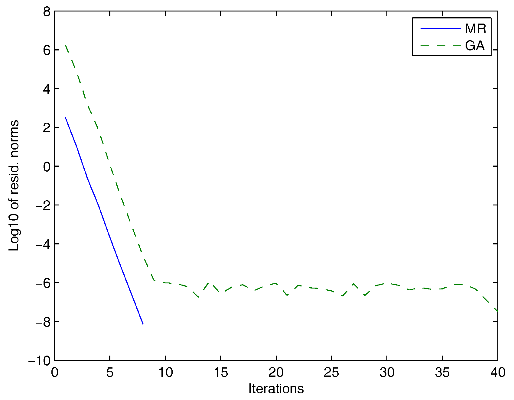
on the unit square $[0,1]\times [0,1]$ with homogeneous Dirichlet boundary conditions. The number of inner grid points in each direction was $n_0$ and $s_0$ for the operators $L_A$ and $L_B$, respectively. The matrices A and B were obtained from the discretization of the operator $L_A$ and $L_B$ with the dimensions $n=n_0^2$ and $s=s_0^2$, respectively. The discretization of the operator $L_A\left(u\right)$ and $L_B\left(u\right)$ yields matrices extracted from the Lyapack package [30] using the command fdm_2d_matrix and denoted as A = fdm(n0,’f_1(x,y)’,’f_2(x,y)’,’f(x,y)’). In this example, $n=10,000$ and $s=4900$, respectively, and are named as $A=\mathrm{fdm}(n0,f_1(x,y),f_2(x,y),f(x,y))$ and $B=\mathrm{fdm}(s0,g_1(x,y),g_2(x,y),g(x,y))$ with $f_1(x,y)=-e^{xy}$, $f_2(x,y)=-sin\left(xy\right)$, $f(x,y)=y^2$, $g_1(x,y)=-100e^x$, $g_2(x,y)=-12xy$ and $g(x,y)=\sqrt{x^2+y^2}$. For this experiment, we used $r=3$.

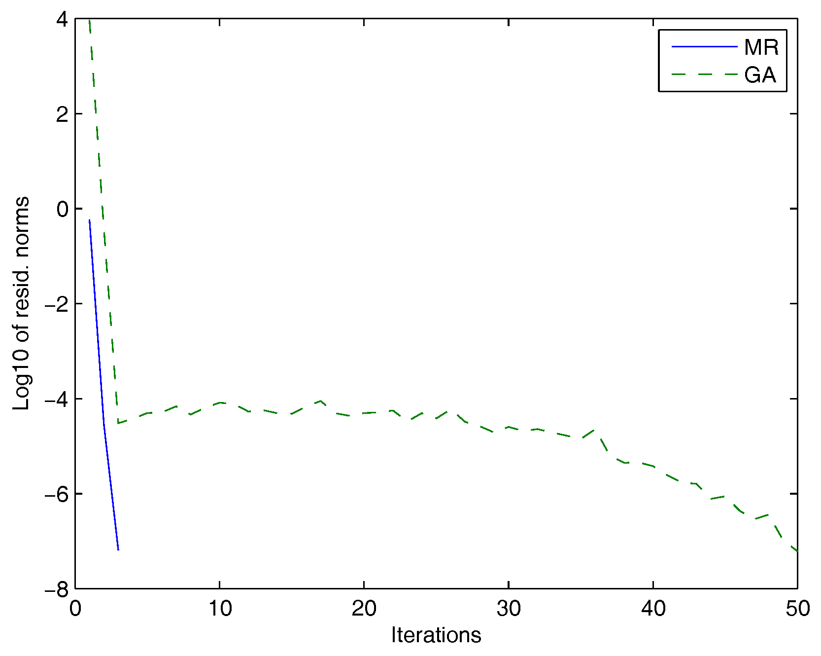
In Figure 1, we plotted the Frobenius norms of the residuals versus the number of iterations for the MR and the GAs.

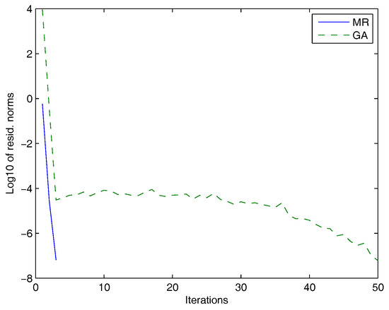
Figure 1. Galerkin approach (GA): dashed line, minimal residual (MR): solid line.

In Table 1, we compared the performances of the MR method and the GA. For both methods, we listed the residual norms, the maximum number of iteration and the corresponding execution time.

Table 1. Results for Example 1.

Test Problem	Method	Iterations	Residual Norm	Times (s)
$n=8100$, $s=3600$, $r=2$	GA	43	7.56 × 10${}^{-8}$	4.80
	MR	3	$1.46\times {10}^{-8}$	1.87
$n=$ 10,000, $s=4900$, $r=4$	GA	45	$4.99\times {10}^{-8}$	26.52
	MR	3	$6.28\times {10}^{-8}$	3.75
$n=$ 12,100, $s=7900$, $r=3$	GA	49	$8.93\times {10}^{-8}$	12.96
	MR	3	$4.98\times {10}^{-8}$	3.63

Example 2.

For the second set of experiments, we considered matrices from the University of Florida Sparse Matrix Collection [31] and from the Harwell Boeing Collection (http://math.nist.gov/MatrixMarket).

In Figure 2, we used the matrices A = pde2961 and B = fdm$(s0,100e^x,12xy,\sqrt{x^2+y^2})$ with dimensions $n=2961$ and $s=3600$, respectively, and $r=3$.

Figure 2. GA: dashed line, MR: solid line.

In Figure 3, we used the matrices A=Themal and B=fdm$(s_0,e^{xy},sin\left(xy\right),x^2-y^2)$ with dimensions $n=3456$ and $s=6400$, respectively, and $r=3$.

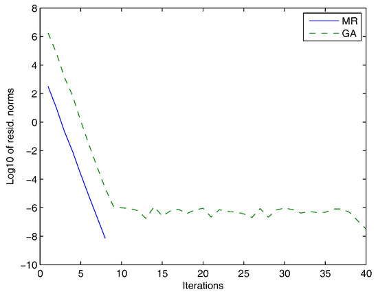
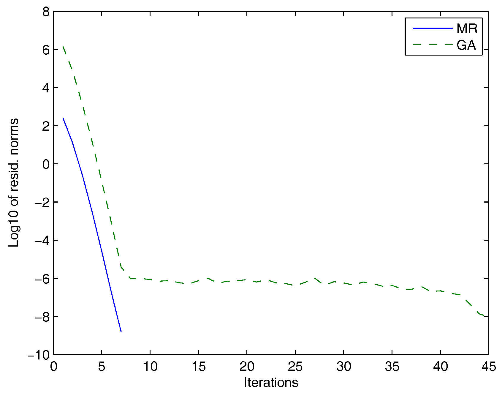
Figure 3. GA: dashed line, MR: solid line.

In Table 2, we compared the performances of the MR method and the GA. For both methods, we listed the residual norms, the maximum number of iterations and the corresponding execution time.

Table 2. Results for Example 5.2.

Test Problem	Method	Iterations	Residual Norm	Time (s)
$n=2961$, $s=3600$, $r=2$, A = pde2961	GA	45	$9.10\times {10}^{-9}$	3.7440
and B = fdm$(s_0,100e^x,12xy,\sqrt{x^2+y^2})$	MR	7	$1.54\times {10}^{-9}$	1.0296
$n=3456$, $s=8100$, $r=3$, A = Thermal	GA	40	$3.27\times {10}^{-8}$	10.1245
and B = fdm$(e^x,sin\left(xy\right),x^2-y^2)$	MR	8	$7.29\times {10}^{-9}$	7.3008

6. Conclusions

We presented in this paper two iterative methods for computing numerical solutions for large scale Stein matrix equations with low rank right-hand sides. The proposed methods are based on projection onto extended block Krylov subspaces with a Galerkin or a minimal residual approach. The approximate solutions are given as products of two low rank matrices and allow for saving memory for large problems. The numerical experiments show that the proposed Krylov-based methods are effective for large and sparse matrices.

References

- Bouhamidi, A.; Heyouni, M.; Jbilou, K. Block Arnoldi-based methods for large scale discrete-time algebraic Riccati equations. J. Comput. Appl. Math. 2011, 236, 1531–1542. [Google Scholar] [CrossRef]
- Bouhamidi, A.; Jbilou, K. Sylvester Tikhonov-regularization methods in image restoration. J. Comput. Appl. Math. 2007, 206, 86–98. [Google Scholar] [CrossRef]
- Zhou, B.; Lam, J.; Duan, G.-R. On Smith-type iterative algorithms for the Stein matrix equation. Appl. Math. Lett. 2009, 22, 1038–1044. [Google Scholar] [CrossRef]
- Zhou, B.; Lam, J.; Duan, G.-R. Toward solution of matrix equation X = Af (X)B + C. Linear Algebra Appl. 2011, 435, 1370–1398. [Google Scholar] [CrossRef]
- Zhou, B.; Duan, G.-R.; Lam, J. Positive definite solutions of the nonlinear matrix equation. Appl. Math. Comput. 2013, 219, 7377–7391. [Google Scholar] [CrossRef]
- Li, Z.-Y.; Zhou, B.; Lam, J. Towards positive definite solutions of a class of nonlinear matrix equations. Appl. Math. Comput. 2014, 237, 546–559. [Google Scholar] [CrossRef]
- Van Dooren, P. Gramian Based Model Reduction of Large-Scale Dynamical Systems. In Numerical Analysis; Chapman and Hall/CRC Press: London, UK, 2000; pp. 231–247. [Google Scholar]
- Datta, B.N. Numerical Methods for Linear Control Systems; Academic Press: New York, NY, USA, 2003. [Google Scholar]
- Datta, B.N.; Datta, K. Theoretical and computational aspects of some linear algebra problems in control theory. In Computational and Combinatorial Methods in Systems Theory; Byrnes, C.I., Lindquist, A., Eds.; Elsevier: Amsterdam, The Netherlands, 1986; pp. 201–212. [Google Scholar]
- Calvetti, D.; Levenberg, N.; Reichel, L. Iterative methods for X − AXB = C. J. Comput. Appl. Math. 1997, 86, 73–101. [Google Scholar] [CrossRef]
- Bartels, R.H.; Stewart, G.W. Solution of the matrix equation A X + X B = C, Algorithm 432. Commun. ACM 1972, 15, 820–826. [Google Scholar] [CrossRef]
- Golub, G.H.; Nash, S.; van Loan, C. A Hessenberg Schur method for the problem AX + XB = C. IEEE Trans. Autom. Control 1979, 24, 909–913. [Google Scholar] [CrossRef]
- Simoncini, V. Computational methods for linear matrix equations. SIAM Rev. 2016, 58, 377–441. [Google Scholar] [CrossRef]
- Agoujil, S.; Bentbib, A.H.; Jbilou, K.; Sadek, E.L.M. A minimal residual norm method for large-scale Sylvester matrix equations. Elect. Trans. Numer. Anal. 2014, 43, 45–59. [Google Scholar]
- Bentbib, A.H.; Jbilou, K.; Sadek, E.M. On some Krylov subspace based methods for large-scale nonsymmetric algebraic Riccati problems. Comput. Math. Appl. 2015, 2555–2565. [Google Scholar] [CrossRef]
- Druskin, V.; Knizhnerman, L. Extended Krylov subspaces: Approximation of the matrix square root and related functions. SIAM J. Matrix Anal. Appl. 1998, 19, 755–771. [Google Scholar] [CrossRef]
- El Guennouni, A.; Jbilou, K.; Riquet, A.J. Block Krylov subspace methods for solving large Sylvester equations. Numer. Algorithms 2002, 29, 75–96. [Google Scholar] [CrossRef]
- Heyouni, M. Extended Arnoldi methods for large low-rank Sylvester matrix equations. Appl. Numer. Math. 2010, 60, 1171–1182. [Google Scholar] [CrossRef]
- Jaimoukha, I.M.; Kasenally, E.M. Krylov subspace methods for solving large Lyapunov equations. SIAM J. Numer. Anal. 1994, 31, 227–251. [Google Scholar] [CrossRef]
- Jbilou, K. Low-rank approximate solution to large Sylvester matrix equations. Appl. Math. Comput. 2006, 177, 365–376. [Google Scholar] [CrossRef]
- Jbilou, K.; Riquet, A.J. Projection methods for large Lyapunov matrix equations. Linear Algebra Appl. 2006, 415, 344–358. [Google Scholar] [CrossRef]
- Lin, Y.; Simoncini, V. Minimal residual methods for large scale Lyapunov equations. Appl. Numer. Math. 2013, 72, 52–71. [Google Scholar] [CrossRef]
- Simoncini, V. A new iterative method for solving large-scale Lyapunov matrix equations. SIAM J. Sci. Comput. 2007, 29, 1268–1288. [Google Scholar] [CrossRef]
- Jagels, C.; Reichel, L. Recursion relations for the extended Krylov subspace method. Linear Algebra Appl. 2011, 434, 1716–1732. [Google Scholar] [CrossRef]
- Heyouni, M.; Jbilou, K. An extended Block Arnoldi algorithm for large-scale solutions of the continuous-time algebraic Riccati equation. Elect. Trans. Numer. Anal. 2009, 33, 53–62. [Google Scholar]
- Saad, Y. Numerical solution of large Lyapunov equations. In Signal Processing, Scattering, Operator Theory and Numerical Methods; Kaashoek, M.A., van Shuppen, J.H., Ran, A.C., Eds.; Birkhaser: Boston, MA, USA, 1990; pp. 503–511. [Google Scholar]
- Bouhamidi, A.; Hached, M.; Heyouni, M.; Jbilou, K. A preconditioned block Arnoldi method for large Sylvester matrix equations. Numer. Linear Algebra Appl. 2011, 20, 208–219. [Google Scholar] [CrossRef]
- Saad, Y. Iterative Methods for Sparse Linear Systems, 2nd ed.; Society for Industrial and Applied Mathematics: Philadelphia, PA, USA, 2003. [Google Scholar]
- Saad, Y.; Yeung, M.; Erhel, J.; Guyomarc’h, F. A deflated version of the conjugate gradient algorithm. SIAM J. Sci. Comput. 2000, 21, 1909–1926. [Google Scholar] [CrossRef]
- Penzl, T. LYAPACK A MATLAB Toolbox for Large Lyapunov and Riccati Equations, Model Reduction Problems, and Linear-Quadratic Optimal Control Problems. Available online: http://www.tu-chemintz.de/sfb393/lyapack (Accessed on 10 June 2016).
- Davis, T. The University of Florida Sparse Matrix Collection, NA Digest, Volume 97, No. 23, 7 June 1997. Available online: http://www.cise.ufl.edu/research/sparse/matrices (Accessed on 10 June 2016).
© 2017 by the authors. Licensee MDPI, Basel, Switzerland. This article is an open access article distributed under the terms and conditions of the Creative Commons Attribution (CC BY) license (http://creativecommons.org/licenses/by/4.0/).