Higher Order Methods for Nonlinear Equations and Their Basins of Attraction

Abstract

In this paper, we have presented a family of fourth order iterative methods, which uses weight functions. This new family requires three function evaluations to get fourth order accuracy. By the Kung–Traub hypothesis this family of methods is optimal and has an efficiency index of 1.587. Furthermore, we have extended one of the methods to sixth and twelfth order methods whose efficiency indices are 1.565 and 1.644, respectively. Some numerical examples are tested to demonstrate the performance of the proposed methods, which verifies the theoretical results. Further, we discuss the extraneous fixed points and basins of attraction for a few existing methods, such as Newton’s method and the proposed family of fourth order methods. An application problem arising from Planck’s radiation law has been verified using our methods.

1. Introduction

One of the best root-finding methods for solving nonlinear scalar equation $f\left(x\right)=0$ is Newton’s method. In recent years, numerous higher order iterative methods have been developed and analyzed for solving nonlinear equations that improve classical methods, such as Newton’s method (NM), Halley’s iteration method, etc., which are respectively given below:

$$x_{n+1}=x_n-\frac{f\left(x_n\right)}{f^{\prime }\left(x_n\right)}$$

(1)

and:

$$x_{n+1}=x_n-\frac{2f\left(x_n\right)f^{\prime }\left(x_n\right)}{2f^{\prime }{\left(x_n\right)}^2-f\left(x_n\right)f^{″}\left(x_n\right)}.$$

(2)

The convergence order of Newton’s method is two, and it is optimal with two function evaluations. Halley’s iteration method has third order convergence with three function evaluations. Frequently, $f^{″}$ is difficult to calculate and computationally more costly, and therefore, $f^{″}$ in Equation (2) is approximated using the finite difference; still, the convergence order and total number function evaluation are maintained [1]. Such a third order method similar to Equation (2) after approximating $f^{″}$ in Halley’s iteration method is given below:

$$y_n=x_n-\beta \frac{f\left(x_n\right)}{f^{\prime }\left(x_n\right)},x_{n+1}=x_n-\frac{2\beta f\left(x_n\right)}{(2\beta -1)f^{\prime }\left(x_n\right)+f^{\prime }\left(y_n\right)},\beta \ne 0.$$

(3)

In the past decade, a few authors have proposed third order methods with three function evaluations free from $f^{″}$; for example, [2,3] and the references therein. The efficiency index (EI) of an iterative method is measured using the formula $p^{\frac{1}{d}}$, where p is the local order of convergence and d is the number of function evaluations per full iteration cycle. Kung–Traub [4] conjectured that the order of convergence of any multi-point without the memory method with d function evaluations cannot exceed the bound $2^{d-1}$, the “optimal order”. Thus, the optimal order for three evaluations per iteration would be four. Jarratt’s method [5] is an example of an optimal fourth order method. Recently, some optimal and non-optimal multi-point methods have been developed in [6,7,8,9,10,11,12,13,14,15] and the references therein. A non-optimal method [16] has been recently rediscovered based on a quadrature formula, which can also be obtained by giving $\beta =\frac{2}{3}$ in Equation (3). In fact, each iterative fixed-point method produces a unique basins of attraction and fractal behavior, which can be used in the evaluation of algorithms [17]. Polynomiography is defined to be the art and science of visualization in the approximation of zeros of complex polynomials, where the created polynomiography images satisfy the mathematical convergence properties of iteration functions.

This paper considers a new family of optimal fourth order methods, which is an improvement of the method given in [16]. We study extraneous fixed points and basins of attraction for two particular cases of the new family of methods and a few equivalent available methods. The rest of the paper is organized as follows. Section 2 presents the development of the methods, their convergence analysis and the extension of new fourth order methods to sixth and twelfth order. Section 3 includes some numerical examples and results for the new family of methods along with some equivalent methods, including Newton’s method. In Section 4, we obtain all possible extraneous fixed points for these methods as a special study. In Section 5, we study basins of attraction for the proposed fourth order methods, Newton’s method and some existing methods. Section 6 discusses an application on Planck’s radiation law problem. Finally, Section 7 gives the conclusions of our work.

2. Development of the Methods and Convergence Analysis

Noor et al. [16] consider the following third order method for the value of $\beta =\frac{2}{3}$ in Equation (3):

$$y_n=x_n-\frac{2}{3}\frac{f\left(x_n\right)}{f^{\prime }\left(x_n\right)},x_{n+1}=x_n-\frac{4f\left(x_n\right)}{f^{\prime }\left(x_n\right)+3f^{\prime }\left(y_n\right)}.$$

(4)

This Method (4) is of order three with three evaluations per full iteration having EI = 1.442. To improve the order of the above method with the same number of function evaluations leading to an optimal method, we propose the following without memory method, which includes weight functions:

$$\begin{array}{c}{y}_n=x_n-\frac{2}{3}\frac{f\left(x_n\right)}{f^{\prime }\left(x_n\right)}\hfill \\ x_{n+1}=x_n-\frac{4f\left(x_n\right)}{f^{\prime }\left(x_n\right)+3f^{\prime }\left(y_n\right)}\times \left(H\left(\tau \right)\times G\left(\eta \right)\right),\hfill \end{array}$$

(5)

where $H\left(\tau \right)$ and $G\left(\eta \right)$ are two weight functions with $\tau =\frac{f^{\prime }\left(y_n\right)}{f^{\prime }\left(x_n\right)}$ and $\eta =\frac{f^{\prime }\left(x_n\right)}{f^{\prime }\left(y_n\right)}$.

2.1. Convergence Analysis

The proofs for Theorems 1 and 2 are worked out with the help of Mathematica.

Theorem 1. 

Let $f:D\subset \mathbb{R}\to \mathbb{R}$ be a sufficiently smooth function having continuous derivatives up to fourth order. If $f\left(x\right)$ has a simple root $x^{*}$ in the open interval D and $x_0$ is chosen in a sufficiently small neighborhood of $x^{*}$, then the family of Method (5) is of local fourth-order convergence, when:

$$H\left(1\right)=G\left(1\right)=1,H^{\prime }\left(1\right)=G^{\prime }\left(1\right)=0,H^{″}\left(1\right)=\frac{5}{8},G^{″}\left(1\right)=\frac{1}{2},|H^{‴}\left(1\right)|=|G^{‴}\left(1\right)|<\infty$$

(6)

and it satisfies the error equation:

$$e_{n+1}=\frac{1}{81}\left(-81c_2{c}_3+9c_4+c_2^3\left(147+32H^{\prime \prime \prime }\left(1\right)-32G^{‴}\left(1\right)\right)\right)e_n^4+O\left(e_n^5\right),$$

where ${\displaystyle c_j=\frac{f^{\left(j\right)}\left(x^{*}\right)}{j!f^{\prime }\left(x^{*}\right)},j=2,3,4,...}$ and $e_n=x_n-x^{*}$.

Proof. 

Taylor expansion of $f\left(x_n\right)$ and $f^{\prime }\left(x_n\right)$ about $x^{*}$ gives:

$$f\left(x_n\right)=f^{\prime }\left(x^{*}\right)\left[e_n+c_2{e}_n^2+c_3{e}_n^3+c_4{e}_n^4+\dots \right]$$

(7)

and:

$$f^{\prime }\left(x_n\right)=f^{\prime }\left(x^{*}\right)\left[1+2c_2{e}_n+3c_3{e}_n^2+4c_4{e}_n^3+\dots \right]$$

(8)

so that:

$$y_n=x-\frac{2}{3}\frac{f\left(x_n\right)}{f^{\prime }\left(x_n\right)}=x^{*}+\frac{e_n}{3}+\frac{2}{3}{c}_2{e}_n^2-\frac{4}{3}\left(c_2^2-c_3\right)e_n^3+\frac{2}{3}\left(4c_2^3-7c_2{c}_3+3c_4\right)e_n^4+\dots .$$

(9)

Again, using Taylor expansion of $f^{\prime }\left(y_n\right)$ about $x^{*}$ gives:

$$f^{\prime }\left(y_n\right)=f^{\prime }\left(x^{*}\right)\left[1+\frac{2}{3}{c}_2{e}_n+\frac{1}{3}\left(4c_2^2+c_3\right)e_n^2+\frac{4}{27}\left(-18c_2^3+27c_2{c}_3+c_4\right)e_n^3+\dots \right].$$

(10)

Using Equations (8) and (10), we have:

$$\tau =1-\frac{4}{3}{c}_2{e}_n+\left(4c_2^2-\frac{8}{3}{c}_3\right)e_n^2-\frac{8}{27}\left(36c_2^3-45c_2{c}_3+13c_4\right)e_n^3+\dots$$

(11)

and:

$$\eta =1+\frac{4}{3}{c}_2{e}_n+\frac{4}{9}\left(-5c_2^2+6c_3\right)e_n^2+\frac{8}{27}\left(8c_2^3-21c_2{c}_3+13c_4\right)e_n^3+\dots$$

(12)

Using Equations (7), (8) and (10), then we have:

$$\frac{4f\left(x_n\right)}{f^{\prime }\left(x_n\right)+3f^{\prime }\left(y_n\right)}=e_n-c_2^2{e}_n^3+\left(3c_2^3-3c_2{c}_3-\frac{1}{9}{c}_4\right)e_n^4+\dots .$$

(13)

Expanding the weight function $H\left(\tau \right)$ and $G\left(\eta \right)$ about 1 using Taylor series, we get:

$$\begin{array}{c}H\left(\tau \right)=H\left(1\right)+(\tau -1)H^{\prime }\left(1\right)+\frac{1}{2}{(\tau -1)}^2{H}^{″}\left(1\right)+\frac{1}{6}{(\tau -1)}^3{H}^{‴}\left(1\right)+O\left(H^{\left(4\right)}\left(1\right)\right),\hfill \\ G\left(\eta \right)=G\left(1\right)+(\eta -1)G^{\prime }\left(1\right)+\frac{1}{2}{(\eta -1)}^2{G}^{″}\left(1\right)+\frac{1}{6}{(\eta -1)}^3{G}^{‴}\left(1\right)+O\left(G^{\left(4\right)}\left(1\right)\right).\hfill \end{array}$$

(14)

Using Equations (13) and (14) in Equation (5), such that the conditions in Equation (6) are satisfied, we obtain:

$$e_{n+1}=\frac{1}{81}\left(-81c_2{c}_3+9c_4+c_2^3\left(147+32H^{‴}\left(1\right)-32G^{‴}\left(1\right)\right)\right)e_n^4+O\left(e_n^5\right).$$

(15)

Equation (15) shows that Method (5) has fourth order convergence. ☐

Note that for each choice of $|H^{‴}\left(1\right)|<\infty$ and $|G^{‴}\left(1\right)|<\infty$ in Equation (15) will give rise to a new optimal fourth order method. Method (5) has efficiency index EI = 1.587, better than Method (4). Two members in the family of Method (5) satisfying Condition (6), with corresponding weight functions, are given in the following:

By choosing $H^{‴}\left(1\right)=G^{‴}\left(1\right)=0$, we get a new Proposed method called as PM1:

$$\begin{array}{c}{y}_n=x_n-\frac{2}{3}\frac{f\left(x_n\right)}{f^{\prime }\left(x_n\right)},\hfill \\ x_{n+1}=x_n-\frac{4f\left(x_n\right)}{f^{\prime }\left(x_n\right)+3f^{\prime }\left(y_n\right)}\left(1+\frac{5}{16}{\left(\tau -1\right)}^2\right)\left(1+\frac{1}{4}{\left(\eta -1\right)}^2\right),\hfill \end{array}$$

(16)

where its error equation is:

$$e_{n+1}=\left(\frac{49}{27}{c}_2^3-c_2{c}_3+\frac{1}{9}{c}_4\right)e_n^4+O\left(e_n^5\right).$$

By choosing $H^{‴}\left(1\right)=0,G^{‴}\left(1\right)=1$, we get another new Proposed method called as PM2:

$$\begin{array}{c}{y}_n=x_n-\frac{2}{3}\frac{f\left(x_n\right)}{f^{\prime }\left(x_n\right)},\hfill \\ x_{n+1}=x_n-\frac{4f\left(x_n\right)}{f^{\prime }\left(x_n\right)+3f^{\prime }\left(y_n\right)}\left(1+\frac{5}{16}{\left(\tau -1\right)}^2\right)\left(1+\frac{1}{4}{\left(\eta -1\right)}^2+\frac{1}{6}{\left(\eta -1\right)}^3\right),\hfill \end{array}$$

(17)

where its error equation is:

$$e_{n+1}=\left(\frac{115}{81}{c}_2^3-c_2{c}_3+\frac{1}{9}{c}_4\right)e_n^4+O\left(e_n^5\right).$$

Remark 1. 

By this way, we can propose many such fourth order methods similar to PM1 and PM2. Further, the methods PM1 and PM2 are equally good, since they have the same order of convergence and efficiency. Based on the analysis done using basins of attraction, we find that PM1 is marginally better than PM2, and hence, we have considered PM1 to propose a higher order method, namely PM3.

2.2. Higher Order Methods

We extend the method PM1 to a new sixth order method called as PM3:

$$\begin{array}{c}{y}_n=x_n-\frac{2}{3}\frac{f\left(x_n\right)}{f^{\prime }\left(x_n\right)},\hfill \\ z_n=x_n-\frac{4f\left(x_n\right)}{f^{\prime }\left(x_n\right)+3f^{\prime }\left(y_n\right)}\left(1+\frac{5}{16}{\left(\tau -1\right)}^2\right)\left(1+\frac{1}{4}{\left(\eta -1\right)}^2\right),\hfill \\ x_{n+1}=z_n-\frac{1}{2}\frac{f\left(z_n\right)}{f^{\prime }\left(x_n\right)}\left(3\eta -1\right).\hfill \end{array}$$

(18)

The following theorem gives the proof of convergence for Method (18).

Theorem 2. 

Let $f:D\subset \mathbb{R}\to \mathbb{R}$ be a sufficiently smooth function having continuous derivatives up to fourth order. If $f\left(x\right)$ has a simple root $x^{*}$ in the open interval D and $x_0$ is chosen in a sufficiently small neighborhood of $x^{*}$, then Method (18) is of local sixth order convergence, and it satisfies the error equation:

$$e_{n+1}=\frac{1}{81}\left(10c_2^2-3c_3\right)\left(49c_2^3-27c_2{c}_3+3c_4\right)e_n^6+O\left(e_n^7\right).$$

Proof. 

Taylor expansion of $f\left(z_n\right)$ about $x^{*}$ gives:

$$\begin{array}{ccc}\hfill f\left(z_n\right)& =& f^{\prime }\left(x^{*}\right)[\left(\frac{49}{27}{c}_2^3-c_2{c}_3+\frac{1}{9}{c}_4\right)e_n^4-\frac{2}{81}\left(403c_2^4-522c_2^{2}c3+81c_3^2+90c_2{c}_4-12c_5\right)e_n^5\hfill \\ & & +\frac{2}{243}(4529c_2^5-8835c_2^3{c}_3+2343c_2^2{c}_4-891c_3{c}_4+135c_2(25c_3^2-3c_5)+63c_6)e_n^6].\hfill \end{array}$$

(19)

By using Equations (8), (12) and (19) in Equation (18), we obtain:

$$e_{n+1}=\frac{1}{81}\left(10c_2^2-3c_3\right)\left(49c_2^3-27c_2{c}_3+3c_4\right)e_n^6+O\left(e_n^7\right).$$

(20)

Equation (20) shows that Method (18) has sixth order convergence. ☐

Babajee et al. [7] improved a sixth order Jarratt method to a twelfth order method. Using their technique, we obtain a new twelfth order method called as PM4:

$$\begin{array}{c}{y}_n=x_n-\frac{2}{3}\frac{f\left(x_n\right)}{f^{\prime }\left(x_n\right)},\hfill \\ z_n=x_n-\frac{4f\left(x_n\right)}{f^{\prime }\left(x_n\right)+3f^{\prime }\left(y_n\right)}\left(1+\frac{5}{16}{\left(\tau -1\right)}^2\right)\left(1+\frac{1}{4}{\left(\eta -1\right)}^2\right),\hfill \\ w_n=z_n-\frac{1}{2}\frac{f\left(z_n\right)}{f^{\prime }\left(x_n\right)}\left(3\eta -1\right),\hfill \\ x_{n+1}=w_n-\frac{f\left(w_n\right)}{f^{\prime }\left(w_n\right)},\hfill \end{array}$$

(21)

where $f^{\prime }\left(w_n\right)$ is approximated as follows: in order to reduce one function evaluation, we replace:

$$\begin{array}{c}{f}^{\prime }\left(w_n\right)\approx \frac{1}{z_n-w_n}(f^{\prime }\left(x_n\right)(z_n-w_n)+2f[w_n,x_n,x_n](z_n-x_n)(w_n-x_n)\hfill \\ +(f[z_n,x_n,x_n]-3f[w_n,x_n,x_n]){(w_n-x_n)}^2),\hfill \\ f[z_n,x_n,x_n]=\frac{f[z_n,x_n]-f^{\prime }\left(x_n\right)}{z_n-x_n},f[z_n,x_n]=\frac{f\left(z_n\right)-f\left(x_n\right)}{z_n-x_n},\hfill \\ f[w_n,x_n,x_n]=\frac{f[w_n,x_n]-f^{\prime }\left(x_n\right)}{w_n-x_n},f[w_n,x_n]=\frac{f\left(w_n\right)-f\left(x_n\right)}{w_n-x_n}.\hfill \end{array}$$

The following theorem is given without proof, which can be worked out with the help of Mathematica.

Theorem 3. 

Let $f:D\subset \mathbb{R}\to \mathbb{R}$ be a sufficiently smooth function having continuous derivatives up to fourth order. If $f\left(x\right)$ has a simple root $x^{*}$ in the open interval D and $x_0$ is chosen in a sufficiently small neighborhood of $x^{*}$, then Method (21) is of local twelfth order convergence, and it satisfies the error equation:

$$e_{n+1}=\frac{1}{6561}\left(10c_2^2-3c_3\right){\left(49c_2^3-27c_2{c}_3+3c_4\right)}^2\left(10c_2^3-3c_2{c}_3+3c_4\right)e_n^{12}+O\left(e_n^{13}\right).$$

Remark 2. 

The efficiency indices for the methods PM3 and PM4 are EI = 1.565 and EI = 1.644, respectively.

2.3. Some Existing Fourth Order Methods

Consider the following fourth order optimal methods for the purpose of comparing results:

Jarratt method (JM) [5]:

$$y_n=x_n-\frac{2}{3}\frac{f\left(x_n\right)}{f^{\prime }\left(x_n\right)},x_{n+1}=x_n-\frac{3f^{\prime }\left(y_n\right)+f^{\prime }\left(x_n\right)}{6f^{\prime }\left(y_n\right)-2f^{\prime }\left(x_n\right)}\frac{f\left(x_n\right)}{f^{\prime }\left(x_n\right)}.$$

(22)

Method of Sharifi-Babajee-Soleymani (SBS1) [12]:

$$\begin{array}{c}{y}_n=x_n-\frac{2}{3}\frac{f\left(x_n\right)}{f^{\prime }\left(x_n\right)},\hfill \\ x_{n+1}=x_n-\frac{f\left(x_n\right)}{4}\left(\frac{1}{f^{\prime }\left(x_n\right)}+\frac{3}{f^{\prime }\left(y_n\right)}\right)\left(1+\frac{3}{8}{\left(\frac{f^{\prime }\left(y_n\right)}{f^{\prime }\left(x_n\right)}-1\right)}^2-\frac{69}{64}{\left(\frac{f^{\prime }\left(y_n\right)}{f^{\prime }\left(x_n\right)}-1\right)}^3+{\left(\frac{f\left(x_n\right)}{f^{\prime }\left(y_n\right)}\right)}^4\right).\hfill \end{array}$$

(23)

Method of Sharifi-Babajee-Soleymani (SBS2) [12]:

$$y_n=x_n-\frac{2}{3}\frac{f\left(x_n\right)}{f^{\prime }\left(x_n\right)},x_{n+1}=x_n-\frac{f\left(x_n\right)}{4}\left(\frac{1}{f^{\prime }\left(x_n\right)}+\frac{3}{f^{\prime }\left(y_n\right)}\right)\left(1+\frac{3}{8}{\left(\frac{f^{\prime }\left(y_n\right)}{f^{\prime }\left(x_n\right)}-1\right)}^2+\frac{1}{81}{\left(\frac{f\left(x_n\right)}{f^{\prime }\left(y_n\right)}\right)}^3\right).$$

(24)

Method of Soleymani-Khratti-Karimi (SKK) [15]:

$$\begin{array}{c}{y}_n=x_n-\frac{2}{3}\frac{f\left(x_n\right)}{f^{\prime }\left(x_n\right)},\hfill \\ x_{n+1}=x_n-\frac{2f\left(x_n\right)}{f^{\prime }\left(x_n\right)+f^{\prime }\left(y_n\right)}\left(1+{\left(\frac{f\left(x_n\right)}{f^{\prime }\left(x_n\right)}\right)}^4\right)\left(2-\frac{7}{4}\frac{f^{\prime }\left(y_n\right)}{f^{\prime }\left(x_n\right)}+\frac{3}{4}{\left(\frac{f^{\prime }\left(y_n\right)}{f^{\prime }\left(x_n\right)}\right)}^2\right).\hfill \end{array}$$

(25)

Method of Singh-Jaiswal (SJ) [14]:

$$\begin{array}{c}{y}_n=x_n-\frac{2}{3}\frac{f\left(x_n\right)}{f^{\prime }\left(x_n\right)},\hfill \\ x_{n+1}=x_n-\left(\frac{17}{8}-\frac{9}{4}\frac{f^{\prime }\left(y_n\right)}{f^{\prime }\left(x_n\right)}+\frac{9}{8}{\left(\frac{f^{\prime }\left(y_n\right)}{f^{\prime }\left(x_n\right)}\right)}^2\right)\left(\frac{7}{4}-\frac{3}{4}\frac{f^{\prime }\left(y_n\right)}{f^{\prime }\left(x_n\right)}\right)\frac{f\left(x_n\right)}{f^{\prime }\left(x_n\right)}.\hfill \end{array}$$

(26)

Method of Sharma-Kumar-Sharma (SKS) [13]:

$$\begin{array}{c}{y}_n=x_n-\frac{2}{3}\frac{f\left(x_n\right)}{f^{\prime }\left(x_n\right)},\hfill \\ x_{n+1}=x_n-\left(-\frac{1}{2}+\frac{9}{8}\frac{f^{\prime }\left(x_n\right)}{f^{\prime }\left(y_n\right)}+\frac{3}{8}\frac{f^{\prime }\left(y_n\right)}{f^{\prime }\left(x_n\right)}\right)\frac{f\left(x_n\right)}{f^{\prime }\left(x_n\right)}.\hfill \end{array}$$

(27)

Furthermore, consider the following non-optimal method found in Divya Jain (DJ) [10]:

$$\begin{array}{c}{y}_n=x_n-\frac{f\left(x_n\right)}{f^{\prime }\left(x_n\right)},\hfill \\ z_n=x_n-\frac{2f\left(x_n\right)}{f^{\prime }\left(x_n\right)+f^{\prime }\left(y_n\right)},\hfill \\ x_{n+1}=z_n-\frac{z_n-x_n}{f\left(z_n\right)-f\left(x_n\right)}f\left(z_n\right).\hfill \end{array}$$

(28)

3. Numerical Examples

In this section, we give numerical results on some test functions to compare the efficiency of the proposed family of methods with some known methods. Numerical computations have been carried out in the MATLAB software, rounding to 500 significant digits. Depending on the precision of the computer, we use the stopping criteria for the iterative process: $error=|x_N-x_{N-1}|<ϵ$, where $ϵ={10}^{-50}$ and N is the number of iterations required for convergence. $d_1$ represents the total number of function evaluations. The computational order of convergence (COC) denoted as ρ is given by (see [18]):

$$\rho =\frac{ln|(x_N-x_{N-1})/(x_{N-1}-x_{N-2})|}{ln|(x_{N-1}-x_{N-2})/(x_{N-2}-x_{N-3})|}.$$

Functions taken for our study are mostly used in the literature [7,11], and their simple zeros are given below:

$$\begin{array}{cc}\hfill f_1\left(x\right)& =sin(2cosx)-1-x^2+e^{sin\left(x^3\right)},x^{*}=-0.7848959876612125352...\hfill \\ \hfill f_2\left(x\right)& =x{e}^{x^2}-{sin}^{2}x+3cosx+5,x^{*}=-1.2076478271309189270...\hfill \\ \hfill f_3\left(x\right)& =x^3+4x^2-10,x^{*}=1.3652300134140968457...\hfill \\ \hfill f_4\left(x\right)& =sin\left(x\right)+cos\left(x\right)+x,x^{*}=-0.4566247045676308244...\hfill \\ \hfill f_5\left(x\right)& =\frac{x}{2}-sinx,x^{*}=1.8954942670339809471...\hfill \\ \hfill f_6\left(x\right)& =\sqrt{x^2+2x+5}-2sinx-x^2+3,x^{*}=2.3319676558839640103...\hfill \\ \hfill f_7\left(x\right)& =\sqrt{x}-cosx,x^{*}=0.6417143708728826583...\hfill \\ \hfill f_8\left(x\right)& =x^2+sin\left(\frac{x}{5}\right)-\frac{1}{4},x^{*}=0.4099920179891371316...\hfill \\ \hfill f_9\left(x\right)& =e^{-x}sinx+log(1+x^2)-2,x^{*}=2.4477482864524245021...\hfill \\ \hfill f_{10}\left(x\right)& =\sqrt{x^3}+sinx-30,x^{*}=9.7165019933652005655...\hfill \end{array}$$

From Table 1 and Table 2, we observe that PM1 and PM2 converge in a lesser number of iterations and with low error when compared to Methods (1) and (4). For equivalent fourth order methods, PM1 and PM2 converge in a lesser number of iterations for certain functions, for example PM2 performs better compared to Method (25) for the functions $f_2,f_7,f_8,f_9$ and $f_{10}$. In terms of the number of iterations for convergence, PM1 and PM2 are equivalent to JM. Table 3 and Table 4 displays the total number of function evaluations ($d_1$) and the computational order of convergence (COC) ρ for the methods taken for our study.

Table 1. Comparison of the results for some known methods and proposed methods.

f	x0	NM (1)		Noor et al. (4)		JM (22)		SBS1 (23)		SBS2 (24)		PM1 (16)
		N	Error	N	Error	N	Error	N	Error	N	Error	N	Error
$f_1$	$-0.9$	7	7.7e – 074	5	2.5e – 093	4	1.6e – 067	4	2.1e – 074	4	4.0e – 063	4	4.4e – 065
	$-0.7$	7	1.0e – 074	5	3.3e – 094	4	1.4e – 070	4	1.2e – 083	4	4.2e – 063	4	7.2e – 066
$f_2$	$-1.7$	9	4.3e – 054	6	7.2e – 051	5	1.4e – 085	5	2.4e – 072	6	4.3e – 179	5	4.2e – 058
	$-1.0$	8	1.1e – 064	6	6.0e – 123	5	2.0e – 199	5	5.0e – 081	5	1.4e – 097	5	3.8e – 116
$f_3$	$1.6$	7	7.7e – 063	5	2.0e – 079	4	2.4e – 065	4	5.3e – 059	4	5.6e – 057	4	1.2e – 059
	$1.0$	8	2.8e – 088	5	5.5e – 056	5	1.4e – 187	5	1.3e – 161	5	2.7e – 135	5	2.5e – 149
$f_4$	$-0.2$	7	6.8e – 096	5	6.5e – 121	4	2.1e – 077	4	1.0e – 058	4	2.9e – 070	4	5.4e – 076
	$-0.6$	6	1.5e – 061	4	6.9e – 052	4	4.3e – 100	4	8.8e – 079	4	2.4e – 090	4	1.2e – 099
$f_5$	$1.6$	8	6.8e – 087	5	5.4e – 055	5	5.7e – 169	5	4.9e – 148	5	5.5e – 124	5	7.9e – 137
	$2.0$	7	1.8e – 080	5	1.0e – 101	4	7.4e – 079	4	1.3e – 096	4	2.9e – 072	4	1.2e – 074
$f_6$	$2.1$	6	1.5e – 055	5	1.2e – 142	4	6.5e – 096	4	2.7e – 062	4	5.3e – 080	4	6.3e – 097
	$2.5$	6	9.6e – 055	5	1.3e – 138	4	4.5e – 094	4	7.1e – 073	4	6.1e – 087	4	7.8e – 096
$f_7$	$0.2$	7	2.0e – 074	5	2.2e – 090	4	8.7e – 063	5	9.5e – 142	4	2.8e – 054	4	2.5e – 060
	$0.9$	7	3.0e – 094	5	7.3e – 121	4	3.5e – 079	4	5.9e – 055	4	1.8e – 073	4	6.9e – 081
$f_8$	$0.2$	8	8.2e – 076	6	2.8e – 143	5	7.4e – 151	5	1.0e – 118	5	1.0e – 100	5	3.8e – 114
	$1.5$	9	2.7e – 074	6	1.5e – 070	5	3.1e – 074	5	1.3e – 104	5	1.8e – 061	5	5.6e – 065
$f_9$	$1.9$	7	2.9e – 088	5	4.5e – 110	4	1.0e – 084	5	4.7e – 119	4	9.7e – 057	4	3.1e – 108
	$2.7$	6	5.9e – 058	5	6.1e – 149	4	5.8e – 102	4	7.8e – 066	4	2.9e – 078	4	1.3e – 100
$f_{10}$	$9.9$	6	9.5e – 059	5	1.9e – 149	4	3.3e – 100	4	7.7e – 072	4	3.1e – 086	4	1.7e – 101
	$9.2$	6	3.1e – 052	5	3.3e – 131	4	1.9e – 078	5	5.3e – 128	4	3.0e – 058	4	9.4e – 079

Table 2. Comparison of the results for some known methods and proposed methods.

f	x0	SKK (25)		SJ (26)		SKS (27)		PM2 (17)
		N	Error	N	Error	N	Error	N	Error
$f_1$	$-0.9$	4	4.6e – 062	4	3.0e – 062	4	9.7e – 064	4	2.7e – 066
	$-0.7$	4	9.9e – 060	4	2.9e – 062	4	5.4e – 064	4	1.5e – 067
$f_2$	$-1.7$	6	6.4e – 147	6	3.9e – 153	6	2.9e – 186	5	6.9e – 075
	$-1.0$	5	1.3e – 075	5	1.9e – 149	5	4.1e – 106	5	9.8e – 127
$f_3$	$1.6$	4	9.6e – 061	4	1.6e – 054	4	4.6e – 057	4	2.0e – 062
	$1.0$	5	9.5e – 102	5	4.2e – 142	5	1.7e – 140	5	1.7e – 157
$f_4$	$-0.2$	4	3.5e – 056	4	2.1e – 074	4	3.0e – 075	4	1.3e – 076
	$-0.6$	4	1.7e – 078	4	5.0e – 099	4	2.2e – 099	4	7.4e – 100
$f_5$	$1.6$	5	3.6e – 101	5	1.0e – 134	5	2.4e – 129	5	1.5e – 143
	$2.0$	4	2.0e – 070	4	1.6e – 070	4	1.2e – 072	4	1.2e – 076
$f_6$	$2.1$	4	3.8e – 063	4	1.3e – 098	4	1.2e – 097	4	1.9e – 096
	$2.5$	4	1.5e – 075	4	2.0e – 099	4	3.2e – 097	4	6.7e – 095
$f_7$	$0.2$	5	4.6e – 159	4	1.2e – 057	4	5.2e – 059	4	1.2e – 061
	$0.9$	4	4.8e – 057	4	1.4e – 084	4	2.8e – 082	4	5.9e – 080
$f_8$	$0.2$	5	1.6e – 082	5	3.7e – 132	5	3.5e – 107	5	1.2e – 120
	$1.5$	6	2.1e – 150	5	3.0e – 054	5	1.2e – 059	5	8.6e – 071
$f_9$	$1.9$	5	3.2e – 126	4	3.1e – 080	4	3.5e – 086	4	5.9e – 089
	$2.7$	4	2.5e – 064	4	5.7e – 099	4	7.6e – 100	4	3.2e – 101
$f_{10}$	$9.9$	4	1.3e – 073	4	7.2e – 104	4	1.9e – 102	4	8.0e – 101
	$9.2$	5	8.0e – 127	4	2.9e – 079	4	5.7e – 079	4	1.3e – 078

Table 3. Total number of function evaluations ($d_1$) and COC (ρ).

f	x0	NM (1)		Noor et al. (4)		JM (22)		SBS1 (23)		SBS2 (24)		PM1 (16)
		d1	ρ	d1	ρ	d1	ρ	d1	ρ	d1	ρ	d1	ρ
$f_1$	$-0.9$	14	1.99	15	2.99	12	3.99	12	4.00	12	3.99	12	3.99
	$-0.7$	14	1.99	15	2.98	12	3.99	12	3.99	12	3.99	12	3.99
$f_2$	$-1.7$	18	2.00	18	2.99	15	4.00	15	4.00	18	3.99	15	3.99
	$-1.0$	16	2.00	18	3.00	15	3.99	15	4.00	15	4.00	15	3.99
$f_3$	$1.6$	14	2.00	15	2.98	12	3.99	12	3.99	12	3.99	12	3.99
	$1.0$	16	1.99	15	2.99	15	4.00	15	3.98	15	3.99	15	3.99
$f_4$	$-0.2$	14	2.00	15	3.00	12	3.99	12	4.00	12	3.99	12	3.99
	$-0.6$	12	2.01	12	3.01	12	3.98	12	4.00	12	3.99	12	3.99
$f_5$	$1.6$	16	1.98	15	3.00	15	4.00	15	3.99	15	3.99	15	3.99
	$2.0$	14	1.99	15	2.99	12	3.99	12	3.98	12	4.00	12	3.99
$f_6$	$2.1$	12	1.99	15	3.00	12	3.99	12	3.99	12	3.99	12	4.00
	$2.5$	12	1.98	15	3.00	12	4.00	12	4.00	12	3.99	12	3.99
$f_7$	$0.2$	14	2.00	15	2.99	12	4.00	15	4.00	12	3.98	12	3.99
	$0.9$	14	2.00	15	2.98	12	3.98	12	3.99	12	4.00	12	4.01
$f_8$	$0.2$	16	2.00	18	3.00	15	3.99	15	3.99	15	4.01	15	3.98
	$1.5$	18	1.99	18	2.99	15	3.99	15	4.00	15	3.98	15	3.99
$f_9$	$1.9$	14	1.98	15	2.99	12	3.98	15	4.00	12	3.99	12	3.99
	$2.7$	12	2.00	15	2.98	12	4.00	12	3.99	12	3.99	12	3.99
$f_{10}$	$9.9$	12	1.99	15	3.00	12	4.00	12	3.98	12	3.99	12	3.99
	$9.2$	12	2.00	15	2.99	12	3.99	15	3.99	12	4.00	12	3.99

Table 4. Total number of function evaluations ($d_1$) and COC (ρ).

f	x0	SKK (25)		SJ (26)		SKS (27)		PM2 (17)
		d1	ρ	d1	ρ	d1	ρ	d1	ρ
$f_1$	$-0.9$	12	3.99	12	3.99	12	3.99	12	3.99
	$-0.7$	12	3.99	12	3.99	12	3.99	12	3.99
$f_2$	$-1.7$	18	3.99	18	3.99	18	3.99	15	3.99
	$-1.0$	15	3.99	15	4.00	15	3.99	15	3.99
$f_3$	1.6	12	3.99	12	4.00	12	3.99	12	4.00
	1.0	15	4.00	15	3.99	15	4.00	15	3.99
$f_4$	$-0.2$	12	4.00	12	4.00	12	3.98	12	3.99
	$-0.6$	12	3.98	12	3.99	12	3.99	12	4.00
$f_5$	1.6	15	3.99	15	3.99	15	3.99	15	3.99
	2.0	12	3.99	12	3.99	12	3.99	12	3.99
$f_6$	2.1	12	3.98	12	4.00	12	3.99	12	3.99
	2.5	12	4.00	12	4.00	12	3.99	12	3.99
$f_7$	0.2	15	3.99	12	3.99	12	3.98	12	3.99
	$0.9$	12	3.98	12	3.98	12	3.99	12	4.00
$f_8$	$0.2$	15	4.01	15	3.98	15	4.00	15	3.98
	$1.5$	18	4.00	15	3.99	15	3.99	15	3.99
$f_9$	$1.9$	15	3.99	12	3.99	12	3.98	12	3.99
	$2.7$	12	3.99	12	4.00	12	3.99	12	3.99
$f_{10}$	$9.9$	12	3.99	12	3.99	12	3.99	12	3.99
	$9.2$	15	3.99	12	3.99	12	3.98	12	3.99

Table 5 displays the results for the “$fzero$” command in MATLAB, where $N_1$ is the number of iterations to find the interval containing the root and $f\left(x_n\right)$ is the error after N number of iterations. For the $fzero$ command, zeros are considered to be points where the function actually crosses, not just touches the x-axis. It is observed that the present methods (PM1 and PM2) converge with a lesser number of total function evaluations than the $fzero$ solver.

Table 5. Results for the $fzero$ command in MATLAB.

f	x0	N1	N	d1	f (xn)	x*
$f_1$	$-0.7$	6	6	19	−1.1102e – 016	−0.7849
$f_2$	$-1.7$	8	7	23	−2.6645e – 015	−1.2076
$f_3$	$1.0$	9	6	25	0	1.3652
$f_4$	$-0.2$	13	6	33	−5.5511e – 017	−0.4566
$f_5$	$1.6$	7	6	21	0	1.8955
$f_6$	$2.1$	5	5	16	8.8818e – 016	2.3320
$f_7$	$0.9$	8	4	20	0	0.6417
$f_8$	$0.2$	12	7	32	−2.7756e – 017	0.4100
$f_9$	$1.9$	8	4	21	0	2.4477
$f_{10}$	$9.2$	3	3	10	0	9.7165

4. A Study on Extraneous Fixed Points

Definition 4. 

A point $z_0$ is a fixed point of R if $R\left(z_0\right)=z_0.$

Definition 5. 

A point $z_0$ is called attracting if $|R^{\prime }\left(z_0\right)|<1$, repelling if $|R^{\prime }\left(z_0\right)|>1$ and neutral if $|R^{\prime }\left(z_0\right)|=1$. If the derivative is also zero, then the point is super attracting.

It is interesting to note that all of the above discussed methods can be written as:

$$x_{n+1}=x_n-G_f\left(x_n\right)u\left(x_n\right),u=\frac{f}{f^{\prime }}.$$

(29)

As per the definition, $x^{*}$ is a fixed point of this method, since $u\left(x^{*}\right)=0$. However, the points $\xi \ne x^{*}$ at which $G_f\left(\xi \right)=0$ are also fixed points of the method, since $G_f\left(\xi \right)=0$; the second term on the right side of Equation (29) vanishes. Hence, these points ξ are called extraneous fixed points.

Moreover, for a general iteration function given by:

$$R_p\left(z\right)=z-G_f\left(z\right)u\left(z\right),z\in \mathbb{C},$$

(30)

the nature of extraneous fixed points can be discussed. Based on the nature of the extraneous fixed points, the convergence of the iteration process will be determined. For more details on this aspect, the paper by Vrcsay et al. [19] will be useful. In fact, they investigated that if the extraneous fixed points are attractive, then the method will give erroneous results. If the extraneous fixed points are repelling or neutral, then the method may not converge to a root near the initial guess.

In this section, we will discuss the extraneous fixed points of each method for the polynomial $z^3-1$. As $G_f$ does not vanish in Theorem 6, there are no extraneous fixed points.

Theorem 6. 

There are no extraneous fixed points for Newton’s Method (1) and Method (4).

Theorem 7. 

There are six extraneous fixed points for Jarratt Method (22).

Proof. 

The extraneous fixed point of Jarratt method for which

$$G_f=\frac{3f^{\prime }\left(y\left(z\right)\right)+f^{\prime }\left(z\right)}{6f^{\prime }\left(y\left(z\right)\right)-2f^{\prime }\left(z\right)}$$

are found. Upon substituting $y\left(z\right)=z-\frac{2f\left(z\right)}{3f^{\prime }\left(z\right)}$, we get the equation $\frac{1+7z^3+19z^6}{2+14z^3+11z^6}=0.$ The extraneous fixed points are found to be $0.411175\pm 0.453532i,-0.598358\pm 0.129321i,0.187183\pm 0.582854i.$ All of these fixed points are repelling (since $|R^{\prime }\left(z_0\right)|>1$). ☐

Theorem 8. 

There are fifty two extraneous fixed points for Method (23).

Proof. 

We found for Method (23),

$$G_f=\left(1+3\frac{f^{\prime }\left(z\right)}{f^{\prime }\left(y\left(z\right)\right)}\right)\left(f^{\prime }\left(z\right)+\frac{69}{64}\frac{{(f^{\prime }\left(z\right)-f^{\prime }\left(y\left(z\right)\right))}^3}{f^{\prime }{\left(z\right)}^2}+\frac{f{\left(z\right)}^4{f}^{\prime }\left(z\right)}{f^{\prime }{\left(y\left(z\right)\right)}^4}+\frac{3}{8}\frac{{(f^{\prime }\left(y\left(z\right)\right)-f^{\prime }\left(z\right))}^2}{f^{\prime }\left(z\right)}\right).$$

The extraneous fixed points are at found to be

$0.385139\pm 0.301563i,-0.453731\pm 0.182759i,0.0685914\pm 0.484322i,-0.461227,0.690937,-1.38146\pm 1.63298i,-0.888193\pm 0.382434i,-0.626419\pm 0.447214i,-0.616918\pm 0.228042i,-0.546519\pm 0.138633i,-0.504031\pm 0.0757213i,-0.483094\pm 0.0349619i,-0.345468\pm 0.598527i,-0.0785635\pm 0.774853i,0.0935008\pm 0.707441i,0.140045\pm 0.571188i,0.177037\pm 0.495057i,0.200558\pm 0.445297i,0.205838\pm 1.20668i,0.229093\pm 0.403647i,0.253758\pm 0.407757i,0.299419\pm 0.396038i,0.365488\pm 0.402274i,0.461153\pm 0.411868i,0.659879\pm 0.470766i,0.704721\pm 0.329989i,1.56532\pm 0.938337i.$

All of these fixed points are repelling (since $|R^{\prime }\left(z_0\right)|>1$). ☐

Theorem 9. 

There are thirty nine extraneous fixed points for Method (24).

Proof. 

For Method (24),

$$G_f=\left(1+3\frac{f^{\prime }\left(z\right)}{f^{\prime }\left(y\left(z\right)\right)}\right)\left(f^{\prime }\left(z\right)++\frac{f{\left(z\right)}^3{f}^{\prime }\left(z\right)}{81f^{\prime }{\left(y\left(z\right)\right)}^3}+\frac{3}{8}\frac{{(f^{\prime }\left(y\left(z\right)\right)-f^{\prime }\left(z\right))}^2}{f^{\prime }\left(z\right)}\right).$$

The extraneous fixed points are at

$0.385139\pm 0.301563i,-0.453731\pm 0.182759i,0.0685914\pm 0.484322i3.98917\pm 6.90945i,-7.97834,0.41942\pm 0.726456i,-0.838839,0.277253\pm 0.480215i,-0.554505,0.46341\pm 0.53288i,-0.693192\pm 0.134885i,0.229782\pm 0.667764i,0.367096\pm 0.467142i,-0.588105\pm 0.0843435i,0.221009\pm 0.551486i,0.280074\pm 0.381388i,-0.470329\pm 0.0518574i,0.190255\pm 0.433246i,0.615945\pm 0.214444i,-0.493687\pm 0.426202i,-0.122258\pm 0.640646i.$

All of these fixed points are repelling (since $|R^{\prime }\left(z_0\right)|>1$). ☐

Theorem 10. 

There are twenty four extraneous fixed points for Method (25).

Proof. 

We found for Method (25),

$$G_f=\left(\frac{1}{1+\frac{f^{\prime }\left(y\left(z\right)\right)}{f^{\prime }\left(z\right)}}\right)\left(f^{\prime }\left(z\right)++\frac{f{\left(z\right)}^4}{f^{\prime }{\left(z\right)}^3}\right)\left(2f^{\prime }\left(z\right)-\frac{7}{4}{f}^{\prime }\left(y\left(z\right)\right)+\frac{3}{4}\frac{f^{\prime }{\left(y\left(z\right)\right)}^2}{f^{\prime }\left(z\right)}\right).$$

The extraneous fixed points are found to be

$0.272187\pm 0.394392i,0.20546\pm 0.432916i,-0.477646\pm 0.0385246i,0.676726\pm 0.202542i,-0.513769\pm 0.484791i,-0.162957\pm 0.687333i,-2.12619\pm 2.22671i,-0.51922\pm 0.277607i,-0.217805\pm 0.487789i,0.210804\pm 0.604566i,0.524089\pm 0.172222i,2.12832\pm 2.00454i.$

All of these fixed points are repelling (since $|R^{\prime }\left(z_0\right)|>1$). ☐

Theorem 11. 

There are eighteen extraneous fixed points for Method (26).

Proof. 

For Method (26),

$$G_f=\left(\frac{17}{8}-\frac{9}{4}\frac{f^{\prime }\left(y\left(z\right)\right)}{f^{\prime }\left(z\right)}+\frac{9}{8}{\left(\frac{f^{\prime }\left(y\left(z\right)\right)}{f^{\prime }\left(z\right)}\right)}^2\right)\left(\frac{7}{4}-\frac{3}{4}\frac{f^{\prime }\left(y\left(z\right)\right)}{f^{\prime }\left(z\right)}\right).$$

The extraneous fixed points are at

$-0.333371\pm 0.577415i,0.666742,0.229257\pm 0.397085i,-0.458515,0.710065\pm 0.231721i,-0.555709\pm 0.499074i,-0.154356\pm 0.730795i,0.275117\pm 0.402579i,-0.486202\pm 0.0369693i,0.211085\pm 0.439548i.$

All of these fixed points are repelling (since $|R^{\prime }\left(z_0\right)|>1$). ☐

Theorem 12. 

There are twelve extraneous fixed points for Method (27).

Proof. 

For Method (27),

$$G_f=\left(-\frac{1}{2}+\frac{9}{8}\frac{f^{\prime }\left(z\right)}{f^{\prime }\left(y\left(z\right)\right)}+\frac{3}{8}\frac{f^{\prime }\left(y\left(z\right)\right)}{f^{\prime }\left(z\right)}\right).$$

The extraneous fixed points are at

$0.289483\pm 0.382811i,0.186782\pm 0.442105i,-0.476265\pm 0.0592945i,0.605298\pm 0.2466i,-0.516211\pm 0.400903i,-0.0890867\pm 0.647503i.$

All of these fixed points are repelling (since $|R^{\prime }\left(z_0\right)|>1$). ☐

Theorem 13. 

There are twenty four extraneous fixed points for Method (16).

Proof. 

For Method (16),

$$G_f=\left(\frac{1}{1+3\frac{f^{\prime }\left(y\left(z\right)\right)}{f^{\prime }\left(z\right)}}\right)\left(f^{\prime }\left(z\right)+\frac{5}{16}\frac{{(f^{\prime }\left(y\left(z\right)\right)-f^{\prime }\left(z\right))}^2}{f^{\prime }\left(z\right)}\right)\left(f^{\prime }\left(z\right)+\frac{1}{4}{f}^{\prime }\left(z\right)\frac{{(f^{\prime }\left(z\right)-f^{\prime }\left(y\left(z\right)\right))}^2}{f^{\prime }{\left(y\left(z\right)\right)}^2}\right).$$

The extraneous fixed points are at

$0.622907\pm 0.52714i,-0.767969\pm 0.275883i,0.145063\pm 0.803023i,0.310217\pm 0.445061i,-0.540543\pm 0.0461255i,0.230326\pm 0.491187i,0.280277\pm 0.377418i,0.186715\pm 0.431436i,-0.466992\pm 0.0540183i,0.602147\pm 0.210285i,-0.483186\pm 0.416332i,-0.118961\pm 0.626617i.$

All of these fixed points are repelling (since $|R^{\prime }\left(z_0\right)|>1$). ☐

Theorem 14. 

There are thirty extraneous fixed points for Method (17).

Proof. 

For Method (17),

$$\begin{array}{ccc}\hfill G_f& =& \left(\frac{1}{1+3\frac{f^{\prime }\left(y\left(z\right)\right)}{f^{\prime }\left(z\right)}}\right)\left(f^{\prime }\left(z\right)+\frac{5}{16}\frac{{(f^{\prime }\left(y\left(z\right)\right)-f^{\prime }\left(z\right))}^2}{f^{\prime }\left(z\right)}\right)\hfill \\ & & \left(f^{\prime }\left(z\right)+\frac{1}{4}{f}^{\prime }\left(z\right)\frac{{(f^{\prime }\left(z\right)-f^{\prime }\left(y\left(z\right)\right))}^2}{f^{\prime }{\left(y\left(z\right)\right)}^2}+\frac{1}{6}{f}^{\prime }\left(z\right)\frac{{(f^{\prime }\left(z\right)-f^{\prime }\left(y\left(z\right)\right))}^3}{f^{\prime }{\left(y\left(z\right)\right)}^3}\right).\hfill \end{array}$$

The extraneous fixed points are at

$0.280277\pm 0.377418i,0.186715\pm 0.431436i,-0.466992\pm 0.0540183i,0.602147\pm 0.210285i,-0.483186\pm 0.416332i,-0.118961\pm 0.626617i,0.701957\pm 0.574647i,-0.848638\pm 0.320589i,0.146681\pm 0.895237i,0.296076\pm 0.447202i,-0.535326\pm 0.0328086i,0.23925\pm 0.48001i,0.414766\pm 0.407081i,0.145159\pm 0.562739i,-0.559926\pm 0.155658i.$

All of these fixed points are repelling (since $|R^{\prime }\left(z_0\right)|>1$). ☐

5. Basins of Attraction

Section 2 and Section 3 discussed methods whose roots are in the real domain, that is $f:D\subset \mathbb{R}\to \mathbb{R}$. The study can be extended to functions defined in the complex plane $f:D\subset \mathbb{C}\to \mathbb{C}$ having complex zeros. From the fundamental theorem of algebra, a polynomial of degree n with real or complex coefficients has n roots, which may or may not be distinct. In such a case, a complex initial guess is needed for the convergence of complex zeros. Note that we need some basic definitions in order to study functions for the complex domain with complex zeros. We give below some definitions required for our study, which are found in [20,21,22]. Let $R:\mathbb{C}\to \mathbb{C}$ be a rational map on the Riemann sphere.

Definition 15. 

For $z\in \mathbb{C}$, we define its orbit as the set $orb\left(z\right)=\{z,R\left(z\right),R^2\left(z\right),...,R^n\left(z\right),...\}.$

Definition 16. 

A periodic point $z_0$ of the period m is such that $R^m\left(z_0\right)=z_0$, where m is the smallest integer.

Definition 17. 

The Julia set of a nonlinear map $R\left(z\right)$ denoted by $J\left(R\right)$ is the closure of the set of its repelling periodic points. The complementary of $J\left(R\right)$ is the Fatou set $F\left(R\right)$.

Definition 18. 

If O is an attracting periodic orbit of period m, we define the basins of attraction to be the open set $A\in \mathbb{C}$ consisting of all points $z\in \mathbb{C}$ for which the successive iterates $R^m\left(z\right),R^{2m}\left(z\right),...$ converge towards some point of O.

Lemma 19. 

Every attracting periodic orbit is contained in the Fatou set of R. In fact, the entire basins of attraction A for an attracting periodic orbit is contained in the Fatou set. However, every repelling periodic orbit is contained in the Julia set.

In the following subsections, we produce some beautiful graphs obtained for the proposed methods and for some existing methods using MATLAB [23,24]. In fact, an iteration function is a mapping of the plane into itself. The common boundaries of these basins of attraction constitute the Julia set of the iteration function, and its complement is the Fatou set. This section is necessary in this paper to show how the proposed methods could be considered in polynomiography. In the following section, we describe the basins of attraction for Newton’s method and some higher order Newton type methods for finding complex roots of polynomials $p_1\left(z\right)=z^3-1$ and $p_2\left(z\right)=z^4-1$.

5.1. Polynomiographs of $p_1\left(z\right)=z^3-1$

We consider the square region $[-2,2]\times [-2,2]$, and in this region, we have 160,000 equally-spaced grid points with mesh $h=0.01$. It is composed of 400 columns and 400 rows, which can be related to the pixels of a computer display, which would represent a region of the complex plane [25]. Each grid point is used as an initial point $z_0$, and the number of iterations until convergence is counted for each point. Now, we draw the polynomiographs of $p_1\left(z\right)=z^3-1$ with roots ${\alpha }_1=1$, ${\alpha }_2=-0.5000-0.8660i$ and ${\alpha }_3=-0.5000+0.8660i$. We assign “red color” if each grid point converges to the root ${\alpha }_1$, “green color” if they converge to the root ${\alpha }_2$ and “blue color” if they converge to the root ${\alpha }_3$ in at most 200 iterations and if $|z_n-{\alpha }_j|<{10}^{-4},j=1,2,3$. In this way, the basins of attraction for each root would be assigned a characteristic color. If the iterations do not converge as per the above condition for some specific initial points, we assign “black color”.

Figure 1a–j shows the polynomiographs of the methods for the cubic polynomial $p_1\left(z\right)$. There are diverging points for the method of Noor et al., SBS1, SBS2 and SKK. All starting points are converging for the methods NM, JM, SJ, SKS, PM1 and PM2. In Table 6, we classify the number of converging and diverging grid points for each iterative method. Note that a point $z_0$ belongs to the Julia set if and only if the dynamics in a neighborhood of $z_0$ displays sensitive dependence on the initial conditions, so that nearby initial conditions lead to wildly different behavior after a number of iterations. For this reason, some of the methods are getting many divergent points. The common boundaries of these basins of attraction constitute the Julia set of the iteration function.

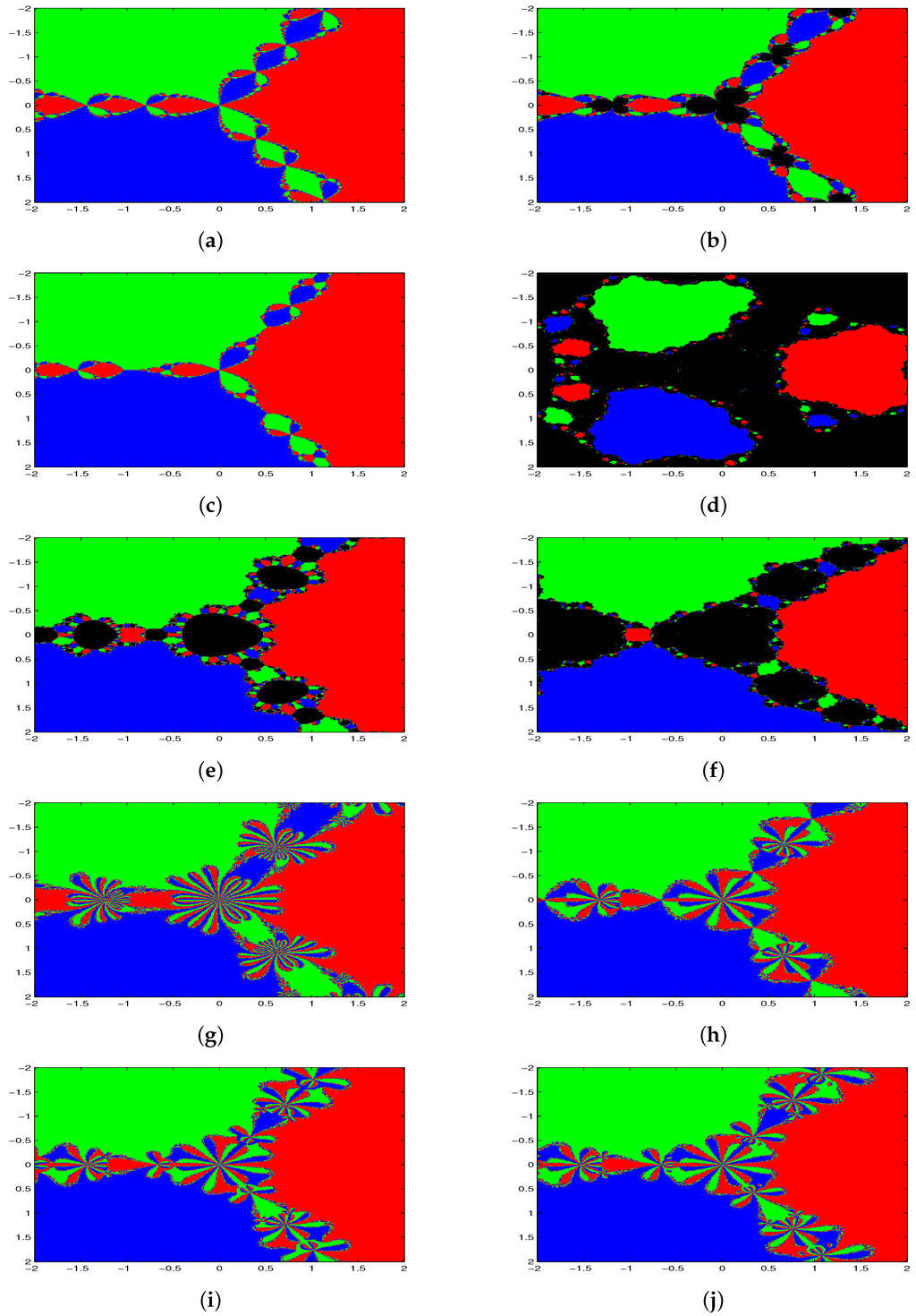
Figure 1. Polynomiographs of $p_1\left(z\right)$. (a) Newton’s method (NM) (1); (b) method of Noor et al. (4); (c) Jarratt method (JM) (22); (d) method of Sharifi et al. (SBS1) (23); (e) method of Sharifi et al. (SBS2) (24); (f) method of Soleymani et al. (SKK) (25); (g) method of Singh et al. (SJ) (26); (h) method of Sharma et al. (SKS) (27); (i) proposed method (PM1) (16); (j) proposed method (PM2) (17).

Table 6. Comparison of convergent and divergent grids for polynomiographs of $p_1\left(z\right)$.

Methods	Convergent Grid Points		Divergent Grid Points
	Real Root (α1)	Complex Roots (α2 and α3)
NM (1)	56,452	103,548	0
Noor et al. (4)	52,372	98,670	8958
JM (22)	56,474	103,526	0
SBS1 (23)	23,174	44,160	92,666
SBS2 (24)	48,018	91,308	20,674
SKK (25)	34,722	82,590	42,688
SJ (26)	52,587	107,143	0
SKS (27)	55,178	104,822	0
PM1 (16)	55,892	104,108	0
PM2 (17)	54,622	105,378	0

5.2. Polynomiographs of $p_2\left(z\right)=z^4-1$

Next, we draw the polynomiographs of $p_2\left(z\right)=z^4-1$ with roots ${\alpha }_1=1$, ${\alpha }_2=-1$, ${\alpha }_3=i$ and ${\alpha }_4=-i$. We assign yellow color if each grid point converges to the root ${\alpha }_1$, red color if they converge to the root ${\alpha }_2$, green color if they converge to the root ${\alpha }_3$ and blue color if they converge to the root ${\alpha }_4$ in at most 200 iterations and if $|z_n-{\alpha }_j|<{10}^{-4},j=1,2,3,4$. Therefore, the basins of attraction for each root would be assigned a corresponding color. If the iterations do not converge as per the above condition for some specific initial points, we assign black color.

Figure 2a–j shows the polynomiographs of the methods for the quartic polynomial $p_2\left(z\right)$. There are diverging points for the method of Noor et al., SBS1, SBS2, SKK, SJ, SKS, PM1 and PM2. All starting points are convergent for NM and JM. In Table 7, we classify the number of converging and diverging grid points for each iterative methods. Furthermore, we observe that the SKS, PM1 and PM2 methods are divergent at a lesser number of grid points than the method of Noor et al., SBS1, SBS2, SKK and SJ. Table 8 shows that the proposed methods are better than or equal to other comparable methods with respect to the number of iterations, computational order convergence and error. All of the methods applied on the cubic and quartic polynomials $p_1\left(z\right)$ and $p_2\left(z\right)$ are convergent with real roots as the starting point.

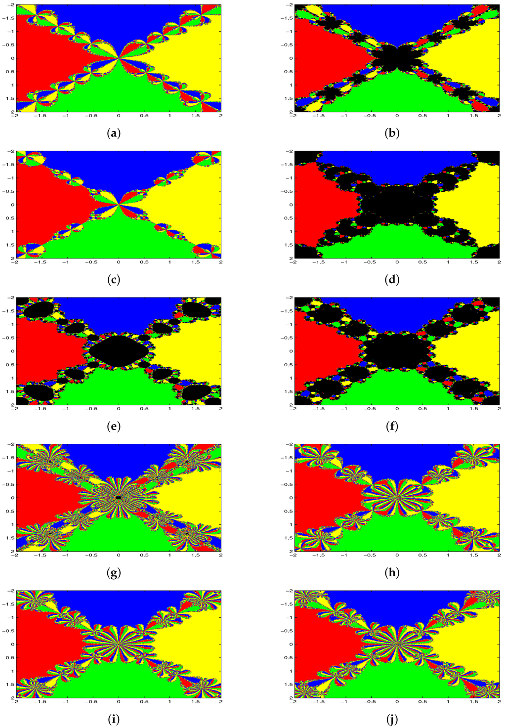
Figure 2. Polynomiographs of $p_2\left(z\right)$. (a) Newton’s method (NM) (1); (b) method of Noor et al. (4); (c) Jarratt method (JM) (22); (d) method of Sharifi et al. (SBS1) (23); (e) method of Sharifi et al. (SBS2) (24); (f) method of Soleymani et al. (SKK) (25); (g) method of Singh et al. (SJ) (26); (h) method of Sharma et al. (SKS) (27); (i) proposed method (PM1) (16); (j) proposed method (PM2) (17).

Table 7. Comparison of convergent and divergent grids for polynomiographs of $p_2\left(z\right)$.

Methods	Convergent Grid Points		Divergent Grid Points
	Real Roots (α1 and α2)	Complex Roots (α3 and α4)
NM (1)	80,010	79,990	0
Noor et al. (4)	68,133	68,120	23,747
JM (22)	80,001	79,999	0
SBS1 (23)	53,792	53,792	52,416
SBS2 (24)	60,098	60,466	39,436
SKK (25)	54,584	54,584	50,832
SJ (26)	79,427	79,427	1146
SKS (27)	79,961	79,959	80
PM1 (16)	79,962	79,979	59
PM2 (17)	79,968	79,954	78

Table 8. Results for polynomials $p_1\left(z\right)$, $p_2\left(z\right)$ with real roots.

Methods	${\mathit{p}}_{\mathbf{1}}\mathbf{\left(}\mathit{z}\mathbf{\right)}\mathbf{=}{\mathit{z}}^{\mathbf{3}}\mathbf{-}\mathbf{1}$				${\mathit{p}}_{\mathbf{2}}\mathbf{\left(}\mathit{z}\mathbf{\right)}\mathbf{=}{\mathit{z}}^{\mathbf{4}}\mathbf{-}\mathbf{1}$
	z0	M	ρ	Error	z0	M	ρ	Error
NM (1)	1.6	9	1.99	3.3751e – 098	0.7	9	1.99	3.1014e – 066
Noor et al. (4)	1.6	6	3.00	3.5077e – 093	0.7	6	3.00	6.2225e – 061
JM (22)	1.6	5	3.99	2.1482e – 108	0.7	6	4.00	2.0563e – 089
SBS1 (23)	1.6	5	4.00	9.3378e – 099	0.7	7	4.00	3.3321e – 110
SBS2 (24)	1.6	5	3.99	9.4664e – 083	0.7	6	3.99	6.2610e – 055
SKK (25)	1.6	5	3.99	1.6780e – 081	0.7	7	3.99	1.7649e – 092
SJ (26)	1.6	5	3.99	8.5156e – 076	0.7	8	3.99	3.9861e – 076
SKS (27)	1.6	5	3.99	9.3481e – 084	0.7	6	3.99	4.7052e – 093
PM1 (16)	1.6	5	3.99	3.1169e – 092	0.7	6	3.99	2.4833e – 099
PM2 (17)	1.6	5	3.99	2.5579e – 102	0.7	6	3.99	3.4840e – 120

From this comparison based on the basins of attractions for cubic and quartic polynomials, we could generally say that NM, JM, PM1 and PM2 are more reliable in solving nonlinear equations. Furthermore, by observing the polynomiographs of $p_1\left(z\right)$ and $p_2\left(z\right)$, we find certain symmetrical patterns for the x-axis and y-axis, where the starting point $z_0$ leads to convergent real or complex pair of roots of the respective polynomials.

6. An Application Problem

To test our methods, we consider the following Planck’s radiation law problem found in [10,26]:

$$\phi \left(\lambda \right)=\frac{8\pi ch{\lambda }^{-5}}{e^{ch/\lambda kT}-1},$$

(31)

which calculates the energy density within an isothermal blackbody. Here, λ is the wavelength of the radiation; T is the absolute temperature of the blackbody; k is Boltzmann’s constant; h is the Planck’s constant; and c is the speed of light. Suppose we would like to determine wavelength λ, which corresponds to maximum energy density $\phi \left(\lambda \right)$. From Equation (31), we get:

$${\phi }^{\prime }\left(\lambda \right)=\left(\frac{8\pi ch{\lambda }^{-6}}{e^{ch/\lambda kT}-1}\right)\left(\frac{\left(ch/\lambda kT\right)e^{ch/\lambda kT}}{e^{ch/\lambda kT}-1}-5\right)=A·B.$$

It can be checked that a maxima for φ occurs when $B=0$, that is when:

$$\left(\frac{\left(ch/\lambda kT\right)e^{ch/\lambda kT}}{e^{ch/\lambda kT}-1}\right)=5.$$

Here, putting $x=ch/\lambda kT$, the above equation becomes:

$$1-\frac{x}{5}=e^{-x}.$$

(32)

Define:

$$f\left(x\right)=e^{-x}-1+\frac{x}{5}.$$

(33)

The aim is to find a root of the equation $f\left(x\right)=0$. Obviously, one of the roots $x=0$ is not taken for discussion. As argued in [26], the left-hand side of Equation (32) is zero for $x=5$ and $e^{-5}\approx 6.74\times {10}^{-3}$. Hence, it is expected that another root of the equation $f\left(x\right)=0$ might occur near $x=5$. The approximate root of the Equation (33) is given by $x^{*}\approx 4.96511423174427630369$. Consequently, the wavelength of radiation (λ) corresponding to which the energy density is maximum is approximated as:

$$\lambda \approx \frac{ch}{\left(kT\right)4.96511423174427630369}.$$

We apply the methods NM, DJ, PM1, PM2, PM3 and PM4 to solve Equation (33) and compared the results in Table 9 and Table 10. From these tables, we note that the root $x^{*}$ is reached faster by the method PM4 than by other methods. This is due to the fact that PM4 has the highest efficiency index EI = 1.644.

Table 9. Comparison of the results.

x0	NM (1)				DJ (28)				PM1 (16)
	N	d1	ρ	Error	N	d1	ρ	Error	N	d1	ρ	Error
4.0	7	14	2.00	1.4e – 101	4	16	4.00	3.3e – 086	4	12	3.99	2.2e – 069
4.5	6	12	1.99	4.5e – 063	4	16	4.00	9.1e – 110	4	12	3.99	2.1e – 093
5.0	6	12	2.00	1.4e – 101	4	16	3.99	8.5e – 185	4	12	3.99	1.3e – 168
5.5	6	12	1.99	5.4e – 066	4	16	4.00	9.9e – 112	4	12	3.99	1.6e – 095

Table 10. Comparison of the results.

x0	PM2 (17)				PM3 (18)				PM4 (21)
	N	d1	ρ	Error	N	d1	ρ	Error	N	d1	ρ	Error
4.0	4	12	3.99	1.4e – 069	4	16	5.99	3.3e – 224	3	15	12.11	7.7e – 144
4.5	4	12	3.99	1.6e – 093	4	16	5.99	3.3e – 306	3	15	12.03	6.4e – 198
5.0	4	12	3.99	1.1e – 168	3	12	5.99	3.7e – 093	3	15	12.00	0
5.5	4	12	3.99	1.4e – 095	3	12	5.95	3.2e – 052	3	15	11.96	3.2e – 203

Results for the $fzero$ command in MATLAB for this application problem are given in Table 11.

Table 11. Results for Planck’s radiation law problem in $fzero$.

x0	N1	N	d1	f (xn)	x*
$4.0$	8	6	23	1.1102e – 016	4.9651
$4.5$	5	5	16	−1.1102e – 016	4.9651
$5.0$	1	4	6	1.1102e – 016	4.9651
$5.5$	5	5	15	−1.1102e – 016	4.9651

7. Conclusions

In this work, we have proposed a family of fourth order methods using weight functions. The fourth order methods are found to be optimal as per the Kung–Traub conjuncture. Further, we have extended one of the methods to sixth and twelfth order methods with four and five function evaluations, respectively. The extraneous fixed points for the fourth order methods and for some existing methods are discussed in detail. By analysis using basins of attraction, our methods PM1 and PM2 are found to be superior to the methods of Noor et al. [16], SBS1, SBS2, SKK and SJ; specifically, the methods of SBS1, SBS2 and SKK are very badly scaled in both cubic and quartic polynomials. Moreover, PM1 and PM2 are better than other compared methods, except Newton’s method and Jaratt’s method, which perform equally well. We have also verified our methods (PM1, PM2, PM3, PM4), NM and DJ on Planck’s radiation law problem, and the results show that PM4 is more efficient than other compared methods.

References

- Ezquerro, J.A.; Hernandez, M.A. A uniparametric halley-type iteration with free second derivative. Int. J. Pure Appl. Math. 2003, 6, 99–110. [Google Scholar]
- Babajee, D.K.R.; Dauhoo, M.Z. An Analysis of the Properties of the Variants of Newton’s Method with Third Order Convergence. Appl. Math. Comput. 2006, 183, 659–684. [Google Scholar] [CrossRef]
- Chun, C.; Yong-Il, K. Several new third-order iterative methods for solving nonlinear equations. Acta Appl. Math. 2010, 109, 1053–1063. [Google Scholar] [CrossRef]
- Kung, H.T.; Traub, J.F. Optimal order of one-point and multipoint iteration. J. Assoc. Comput. Mach. 1974, 21, 643–651. [Google Scholar] [CrossRef]
- Jarratt, P. Some efficient fourth order multipoint methods for solving equations. BIT Numer. Math. 1969, 9, 119–124. [Google Scholar] [CrossRef]
- Ardelean, G. A new third-order newton-type iterative method for solving nonlinear equations. Appl. Math. Comput. 2013, 219, 9856–9864. [Google Scholar] [CrossRef]
- Babajee, D.K.R.; Madhu, K.; Jayaraman, J. A family of higher order multi-point iterative methods based on power mean for solving nonlinear equations. Afr. Mat. 2015. [Google Scholar] [CrossRef]
- Cordero, A.; Hueso, J.L.; Martinez, E.; Torregrosa, J.R. Efficient three-step iterative methods with sixth order convergence for nonlinear equations. Numer. Algor. 2010, 53, 485–495. [Google Scholar] [CrossRef]
- Cordero, A.; Hueso, J.L.; Martinez, E.; Torregrosa, J.R. A family of iterative methods with sixth and seventh order convergence for nonlinear equations. Math. Comput. Model. 2010, 52, 1490–1496. [Google Scholar] [CrossRef]
- Jain, D. Families of newton-like methods with fourth-order convergence. Int. J. Comput. Math. 2013, 90, 1072–1082. [Google Scholar] [CrossRef]
- Madhu, K.; Jayaraman, J. Class of modified Newton’s method for solving nonlinear equations. Tamsui Oxf. J. Inf. Math. Sci. 2014, 30, 91–100. [Google Scholar]
- Sharifi, M.; Babajee, D.K.R.; Soleymani, F. Finding the solution of nonlinear equations by a class of optimal methods. Comput. Math. Appl. 2012, 63, 764–774. [Google Scholar] [CrossRef]
- Sharma, J.R.; Kumar, G.R.; Sharma, R. An efficient fourth order weighted-newton method for systems of nonlinear equations. Numer. Algor. 2013, 62, 307–323. [Google Scholar] [CrossRef]
- Singh, A.; Jaiswal, J.P. Several new third-order and fourth-order iterative methods for solving nonlinear equations. Int. J. Eng. Math. 2014, 2014, 828409. [Google Scholar] [CrossRef]
- Soleymani, F.; Khratti, S.K.; Karimi, V.S. Two new classes of optimal Jarratt-type fourth-order methods. Appl. Math. Lett. 2011, 25, 847–853. [Google Scholar] [CrossRef]
- Noor, M.A.; Waseem, M. Some iterative methods for solving a system of nonlinear equations. Comput. Math. Appl. 2009, 57, 101–106. [Google Scholar] [CrossRef]
- Kalantari, B. Polynomial Root-Finding and Polynomiography; World Scientific Publishing Co. Pte. Ltd.: Singapore, 2009. [Google Scholar]
- Cordero, A.; Torregrosa, J.R. Variants of Newton’s method using fifth-order quadrature formulas. Appl. Math. Comput. 2007, 190, 686–698. [Google Scholar] [CrossRef]
- Vrscay, E.R.; Gilbert, W.J. Extraneous fixed points, basin boundaries and chaotic dynamics for Schroder and Konig rational iteration functions. Numer. Math. 1988, 52, 1–16. [Google Scholar] [CrossRef]
- Amat, S.; Busquier, S.; Plaza, S. Review of some iterative root-finding methods from a dynamical point of view. Sci. Ser. A Math. Sci. 2004, 10, 3–35. [Google Scholar]
- Blanchard, P. Complex Analytic Dynamics on the Riemann sphere. Bull. Am. Math. Soc. 1984, 11, 85–141. [Google Scholar] [CrossRef]
- Scott, M.; Neta, B.; Chun, C. Basin attractors for various methods. Appl. Math. Comput. 2011, 218, 2584–2599. [Google Scholar] [CrossRef]
- Chicharro, F.I.; Cordero, A.; Torregrosa, J.R. Drawing Dynamical and Parameters Planes of Iterative Families and Methods. Sci. World J. 2013. [Google Scholar] [CrossRef] [PubMed]
- Introduction to Computational Engineering. Available online: http://www.caam.rice.edu (accessed on 10 May 2015).
- Soleymani, F.; Babajee, D.K.R.; Sharifi, M. Modified jarratt method without memory with twelfth-order convergence. Ann. Univ. Craiova Math. Comput. Sci. Ser. 2012, 39, 21–34. [Google Scholar]
- Bradie, B. A Friendly Introduction to Numerical Analysis; Pearson Education Inc.: New Delhi, India, 2006. [Google Scholar]
© 2016 by the authors; licensee MDPI, Basel, Switzerland. This article is an open access article distributed under the terms and conditions of the Creative Commons by Attribution (CC-BY) license (http://creativecommons.org/licenses/by/4.0/).